SUPER-GZK NEUTRINOS

Abstract

The sources and fluxes of superGZK neutrinos, $E>10^{20}$ eV, are discussed. The fluxes of cosmogenic neutrinos, i.e. those produced by ultra-high energy cosmic rays (UHECR) interacting with CMB photons, are calculated in the models, which give the good fit to the observed flux of UHECR. The best fit given in no-evolutionary model with maximum acceleration energy $E_{\rm max}=1\times 10^{21}$ eV results in very low flux of superGZK neutrinos an order of magnitude lower than the observed flux of UHECR. The predicted neutrino flux becomes larger and observable by next generation detectors at energies $10^{20}-10^{21}$ eV in the evolutionary models with $E_{\rm max}=1\times 10^{23}$ eV. The largest cosmogenic neutrino flux is given in models with very flat generation spectrum, e.g. $\propto E^{-2}$. The neutrino energies are naturally high in the models of superheavy dark matter and topological defects. Their fluxes can also be higher than those of cosmogenic neutrinos. The largest fluxes are given by mirror neutrinos, oscillating into ordinary neutrinos. Their fluxes obey some theoretical upper limit which is very weak, and in practice these fluxes are most efficiently limited now by observations of radio emission from neutrino-induced showers.

INFN, Laboratori Nazionali del Gran Sasso,
67010 Assergi (AQ) Italy

1 Introduction

The abbreviation ‘SuperGZK neutrinos’ implies neutrinos with energies above the Greisen-Zatsepin-Kuzmin ^?) cutoff $E_{\rm GZK}\sim 5\times 10^{19}$ eV. Soon after theoretical discovery of the GZK cutoff, it has been realized that this phenomenon is accompanied by a flux of UHE neutrinos, which in some models can be very large ^?). In 80s it was understood that topological defects can produce unstable superheavy particles with masses up to the GUT scale ^?) and neutrinos with tremendous energies can emerge due to this process ^?).

It has been proposed that SuperGZK neutrinos can be detected observing the horizontal Extensive Air Showers (EAS) ^?). The exciting prospects for detection of SuperGZK neutrinos have appeared with the ideas of space detection, e.g. in the projects EUSO^?) and OWL^?). The basic idea of detection can be explained by example of EUSO.

The superGZK neutrino entering the Earth atmosphere in near-horizontal direction produces an EAS. The known fraction of its energy, which reaches 90% , is radiated in form of isotropic fluorescent light. An optical telescope from a space observatory detects this light. Since the observatory is located at very large height ($\sim 400$ km) in comparison with thickness of the atmosphere, the fraction of detected flux is known, and thus this is the calorimetric experiment (absorption of light in the upward direction is small). A telescope with diameter 2.5 m controls the area $\sim 10^{5}$ km² and has a threshold for EAS detection $E_{\rm th}\sim 1\times 10^{20}$ eV.

The very efficient method of superGZK neutrino detection is given by observations of radio emission by neutrino-induced showers in ice, salt and lunar regolith. This method has been originally suggested by G. Askaryan in 60s ^?). Propagating in the matter the shower acquires excessive negative electric charge due to involvement of the matter electrons in knock-on process. The coherent Cerenkov radiation of these electrons produces the radio pulse. Recently this method has been confirmed in the laboratory measurements ^?). There were several searches for such radiation from neutrino-induced showers in the Antarctic and Greenland ice and in the lunar regolith. In all cases the radio-emission can be observed only for neutrinos of extremely high energies. The upper limits on the flux of these neutrinos have been obtained: in GLUE experiment ^?) by radiation from the moon, in FORTE experiment ^?) by radiation from the Greenland ice and in RICE experiment ^?) from the Antarctic ice.

The characteristic feature of the detection methods described above is the high energy threshold, typically $E\mathrel{\mathop{\kern 0.0pt\hbox to0.0pt{\raise 0.86108pt\hbox{$>$}\hss}}\lower 3.87495pt\hbox{\kern-1.90002pt$\sim$}}1\times 10^{19}-1\times 10^{20}$ eV. How neutrinos of these energies can be produced?

The most conservative mechanism of superGZK neutrino production is $p\gamma$ mechanism of collisions of accelerated protons/nuclei with low-energy CMB photons. To provide neutrinos with energies higher that $1\times 10^{20}$ eV the accelerated protons must have energies higher (or much higher) than $2\times 10^{21}$ eV. For shock acceleration this energy can reach optimistically $1\times 10^{21}$ eV. One has raise his hopes on less developed ideas of acceleration such as acceleration in strong e-m waves, exotic plasma mechanisms of acceleration and unipolar induction.

The top-down scenarios can easily provide neutrinos with energies higher and much higher than $1\times 10^{20}$ eV. The idea common for many mechanisms is given by existence of superheavy particles with very large masses up to GUT scale. In Grand Unified Theories (GUT) these particles (gauge bosons and higgses) are short-lived. In the cosmic space they are produced by Topological Defects (TDs). The decay of these particles results in the parton cascade, which is terminated by production of pions and other hadrons. Neutrinos are produced in their decays.

The superheavy particles are naturally produced at post-inflationary stage of the universe. The most reliable mechanism of production is gravitational one. The masses of such particles can reach $10^{13}-10^{14}$ GeV. Protecting by some symmetry (e.g. gauge symmetry or discrete gauge symmetry like R-parity in supersymmetry), these particles can survive until present cosmological epoch and produce neutrinos in the decays or annihilation.

2 Upper limits on superGZK neutrino flux

There are two different upper limits on UHE neutrino fluxes: cascade upper limit ^?) and cosmic ray upper limits (Waxman-Bahcall ^?) and Mannheim-Protheroe-Rachen ^?)). The cosmic ray upper limits are not relevant for superGZK neutrinos because this limit is not valid for top-down scenarios and it is automatically satisfied for cosmogenic neutrinos, since their fluxes are calculated in the models which explain the observed UHECR.

The cascade upper limit on HE and UHE neutrino fluxes ^?,?) is provided due to e-m cascades initiated by HE photons or electrons which always accompany production of neutrinos. Colliding with the target photons, a primary photon or electron produce e-m cascade due to reactions $\gamma+\gamma_{\rm tar}\to e^{+}+e^{-}$, $e+\gamma_{\rm tar}\to e^{\prime}+\gamma^{\prime}$, etc (see Fig. 1).

Figure 1: Developing of e-m cascade in collisions with background target (t) photons.

The standard case is given by production of HE neutrinos in extragalactic space, where cascade develops due to collisions with CMB photons ($\gamma_{\rm tar}=\gamma_{\rm CMB}$). In case the neutrino production occurs in a galaxy, the accompanying photon can either freely escapes from a galaxy and produce cascade in extragalactic space, or produce cascade on the background radiation (e.g. infra-red) within the galaxy. In the latter case the galaxy should be transparent for the cascade photons in the range 10  MeV - 100 GeV.

The spectrum of the cascade photons is calculated ^?,?,?): in low energy part it is $\propto E^{-3/2}$, at high energies $\propto E^{-2}$ with a cutoff at some energy $\epsilon_{\gamma}$. The energy of transition between two regimes is given approximately by $\epsilon_{c}\approx(\epsilon_{t}/3)(\epsilon_{\gamma}/m_{e})^{2}$, where $\epsilon_{t}$ is the mean energy of the target photon. In case the cascade develops in extragalactic space $\epsilon_{t}=6.35\times 10^{-4}$ eV, $\epsilon_{\gamma}\sim 100$ GeV (absorption on optical radiation), and $\epsilon_{c}\sim 8$ MeV. The cascade spectrum is very close to the EGRET observations in the range 3 MeV - 100 GeV ^?). The observed energy density in this range is $\omega_{\rm EGRET}\approx(2-3)\times 10^{-6}$ eV/cm³. The upper limit on HE neutrino flux $J_{\nu}(>E)$ is given by chain of the following inequalities

$$\omega_{\rm cas}>\frac{4\pi}{c}\int_{E}^{\infty}EJ_{\nu}(E)dE>\frac{4\pi}{c}E\int_{E}^{\infty}J_{\nu}(E)dE\equiv\frac{4\pi}{c}EJ_{\nu}(>E),$$

which in terms of the differential neutrino spectrum $J_{\nu}(E)$ results in

$$E^{2}J_{\nu}(E)<\frac{c}{4\pi}\omega_{\rm cas},~{}~{}{\rm with}~{}\omega_{\rm cas}<\omega_{\rm EGRET}.$$ (1)

Unless otherwise is stated, here and everywhere below the neutrino flux $J_{\nu}$ is given as sum of all neutrino flavors.

Eq. (1) gives the rigorous upper limit on the neutrino flux. It is valid for neutrino production by HE protons, by TDs, by annihilation and decays of superheavy particles, i.e. in all cases when neutrinos are produced through decay of pions and kaons. It is valid for production of neutrinos in extragalactic space and in galaxies, if they are transparent for the cascade photons. It holds for arbitrary neutrino spectrum falling down with energy. If one assumes some specific shape of neutrino spectrum, the cascade limit becomes stronger. For example, for $E^{-2}$ neutrino spectrum one immediately obtains

$$E^{2}J_{\nu}(E)\leq\frac{c}{4\pi}\frac{\omega_{\rm cas}}{\ln(E_{\rm max}/E_{\rm min})},$$ (2)

3 Cosmogenic neutrinos

Cosmogenic has a meaning “produced by cosmic rays”.

The most efficient mechanism for production of cosmogenic superGZK neutrinos is given by $p\gamma$ collisions of protons with CMB photons: for $E_{\nu}\mathrel{\mathop{\kern 0.0pt\hbox to0.0pt{\raise 0.86108pt\hbox{$>$}\hss}}\lower 3.87495pt\hbox{\kern-1.90002pt$\sim$}}1\times 10^{20}$ eV the energy of the parent protons $E_{p}\sim 20E_{\nu}$ is enough for photopion production in collisions with CMB photons. The space density of CMB photons (412 cm^-3) is usually much larger than number density of the gas and optical/IR photons in the sources and outside.

We shall reproduce here the historically first calculations ^?) of the diffuse neutrino flux produced by UHE protons colliding with CMB photons.

Consider the universe filled uniformly by UHECR sources with space density $n_{s}$ and UHE proton luminosity $L_{p}$. We assume the cosmological evolution of the sources in the form ${\cal L}={\cal L}_{0}(1+z)^{m}$, where ${\cal L}_{0}=L_{p}n_{s}$ is emissivity at the epoch with redshift $z=0$ and factor $(1+z)^{m}$ describes the evolution.

The production rate of a source is given as

$$Q_{\rm gen}=(\gamma_{g}-2)L_{p}E^{-\gamma_{g}},$$ (3)

where all energies are measured in GeV and $E_{\rm min}$ is assumed to be $\sim 1$ GeV.

The diffuse UHE proton flux can be calculated from particle conservation, assuming the generation energy $E_{g}=E_{g}(E,z)$ due to energy losses and integrating over all epochs of generation:

$$J_{p}(E)=\frac{c}{4\pi}(\gamma_{g}-2){\cal L}_{0}\int dt(1+z)^{m}E_{g}^{-\gamma_{g}}(E,z)dE_{g}/dE.$$ (4)

Unmodified diffuse spectrum is calculated with only adiabatic energy losses included: $E_{g}(E,z)=(1+z)E$ and $dE_{g}/dE=1+z$. Using the connection of cosmological time $t$ and redshift $z$ as $dz/dt=H_{0}(1+z)\lambda(z)$, where

$$\lambda(z)=\sqrt{(1+z)^{3}\Omega_{m}+(1+z)^{2}\Omega_{r}+\Omega_{\Lambda}},$$ (5)

$H_{0}$ is the Hubble constant and $\Omega_{m}$,  $\Omega_{r}$ and $\Omega_{\lambda}$ are cosmological density in units of critical density of non-relativistic dark matter $m$, relativistic dark matter $r$ and that due to vacuum energy density $\Lambda$, respectively, one obtains for the unmodified spectrum of UHE protons:

$$J_{\rm unm}(E)=\frac{c}{4\pi}(\gamma_{g}-2)\frac{{\cal L}_{0}}{H_{0}}E^{-\gamma_{g}}\eta_{\rm ev}(m,z_{\rm max}),$$ (6)

where $\eta_{\rm ev}(m,z_{\rm max},\gamma_{g})$ is the evolutionary factor given by

$$\eta_{\rm ev}(m,z_{\rm max},\gamma_{g})=\int_{0}^{z_{\rm max}}dz(1+z)^{m-\gamma_{g}}/\lambda(z).$$ (7)

It is easy to express the neutrino diffuse flux through unmodified proton flux, assuming that a proton undergoes several collisions with CMB photons:

$$J_{\nu}(E)=\frac{2}{3}\cdot 3\left(\frac{E_{\nu}}{E_{p}}\right)^{\gamma_{g}-1}\frac{1}{1-\alpha^{\gamma_{g}-1}}J_{\rm unm}(E),$$ (8)

where 2/3 accounts for probability of charged pion production, 3 - for 3 neutrinos produced in the chain of pion decay, $E_{\nu}/E_{p}\approx 0.05$ is a fraction of proton energy transferred to neutrino, and $\alpha$ is a fraction of energy lost by the proton in $p\gamma$ collision ($\alpha$ varies from 0.22 in $\Delta$-resonance to 0.5 at extremely high energies); the term with $\alpha$ in Eq. (8) describes approximately the subsequent $p\gamma$ collisions of UHE proton.

The low-energy edge of neutrino spectrum (8) is determined by energy of a proton at epoch $z$, at which the energy loss due to pion production becomes less than that due $e^{+}e^{-}$-pair production.

Neutrino flux given by Eq. (8) strongly depends on the parameters of cosmological evolution of the sources, $m$ and $z_{\rm max}$, as it is seen from Eqs. (6) and (7).

The accuracy of neutrino-flux calculations by method of Ref. ^?) can be compared with exact calculations of Ref. ^?), where all details of $p\gamma$ interaction were included and fluxes were computed for all neutrino flavors separately. The total neutrino moments (yields) $Z_{p\gamma}(\gamma_{g})$ calculated in Ref. ^?) must coincide with the coefficient in front of $J_{\rm unm}(E)$ in the rhs of Eq. (8). For $\gamma_{g}\leq 2.7$ the agreement is indeed 20 - 40 %.

The detailed calculations of UHE neutrino fluxes in the similar models with evolution of the sources and with normalization of the fluxes by the proton component have been performed in Refs. ^?) - ^?). In this paper I will present fluxes calculated ^?) in the BGG models ^?), which describe precisely the observed UHECR spectra, with the dip at $1\times 10^{18}-4\times 10^{19}$ eV as the most prominent feature.

In fact there are several BGG ^?) models which give good fit to UHECR spectra as measured by AGASA, HiRes, Fly’s Eye and Yakutsk detectors. They differ by cosmological evolution of the sources, described by factor $(1+z)^{m}$, by exponent $\gamma_{g}$ of the generation spectrum and by maximum energy of accelerated protons $E_{\rm max}$. The model with the best fit (see ^?)) corresponds to $m=0$ (the non-evolutionary model), with the generation index $\gamma_{g}=2.7$ and $E_{\rm max}=1\times 10^{21}$ eV. Less important assumption is flattening of generation spectrum at $E\leq E_{c}$, with $E_{c}\sim 1\times 10^{18}$ eV, which is needed to describe correctly the mass composition observed at $E\leq 1\times 10^{17}$ eV ^?).

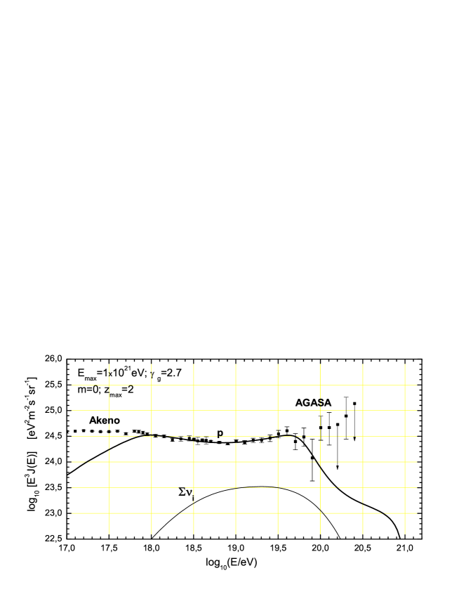
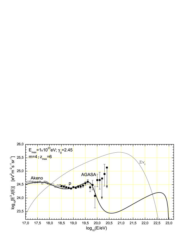
Figure 2: UHE neutrino fluxes ^?) in the non-evolutionary (upper panel) and evolutionary (lower panel) BGG models ^?). In the upper panel the neutrino flux accompanying the observed UHECR flux is shown by curve $\Sigma\nu_{i}$. The following parameters are used in calculations: $m=0$,  $z_{\rm max}=2$,  $\gamma_{g}=2.7$,  $E_{\rm max}=1\times 10^{21}$ eV,  $E_{c}=1\times 10^{18}$ eV and emissivity ${\cal L}_{0}=3.5\times 10^{46}$ erg/Mpc³yr. In the low panel the neutrino flux is maximized by the following choice of parameters: $m=4.0$, $z_{\rm max}=6.0$,  $\gamma_{g}=2.45$ and emissivity ${\cal L}_{0}=1.2\times 10^{46}$ erg Mpc^-1yr^-1. Note that fit to observational data in case of the evolutionary model is worse than for non-evolutionary model.

The spectrum of CR in this model is shown in Fig. 2 (upper panel) in comparison with Akeno-AGASA data. The emissivity of the sources needed to fit the the observed flux is ${\cal L}_{0}=3.5\times 10^{46}$ erg/Mpc³yr, which corresponds to luminosity of a source $L_{p}=3.7\times 10^{43}$ erg/s for space density of the sources (powerful AGN) $n_{s}=3\times 10^{-5}$ Mpc^-3. One can notice the precise agreement with the Akeno-AGASA data at $1\times 10^{18}-8\times 10^{19}$ eV. The explanation of the AGASA excess at $E>1\times 10^{20}$ eV needs the additional CR component of another origin. The calculated neutrino flux is shown by curve $\Sigma\nu_{i}$ for sum of all neutrino flavor. This is the lowest neutrino flux compatible with the observed UHECR flux, because including evolution and increasing $E_{\rm max}$ one increases the neutrino flux. The predicted flux of superGZK neutrinos at $E\mathrel{\mathop{\kern 0.0pt\hbox to0.0pt{\raise 0.86108pt\hbox{$>$}\hss}}\lower 3.87495pt\hbox{\kern-1.90002pt$\sim$}}1\times 10^{20}$ eV is hardly detectable by the methods discussed above.

Thus, the observed UHECR flux does not guarantee the detectable flux of superGZK neutrinos.

In Fig. 2 (lower panel) neutrino flux is maximized for the BGG models, using the cosmological evolution, compatible with the observed UHECR flux, namely ${\cal L}(z)=(1+z)^{m}{\cal L}_{0}$ at $z\leq z_{\rm max}$ with $m=4$, $z_{\rm max}=6$ and ${\cal L}_{0}=1.2\times 10^{46}$ erg/Mpc³yr. Very large $E_{\rm max}=1\times 10^{23}$ eV is used to increase further neutrino flux. Note, that though the local emissivity at $z=0$ is relatively low, it was much larger in the past. The maximum acceleration energy $E_{\rm max}$ cannot be also considered as realistic, and used mostly for illustration of range in the predicted fluxes. Finally, this model fits observed UHECR spectrum worse than non-evolutionary model and has the problems with observed mass composition of cosmic rays at $E<1\times 10^{18}$ eV.

In the evolutionary models with large $m$ and $z_{\rm max}$, which explain the observed UHECR, the fluxes of cosmogenic neutrinos are observable by future detectors.

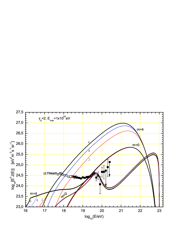
Figure 3: UHE neutrino fluxes ^?) in the evolutionary and non-evolutionary models with proton generation spectrum $\propto E^{-2}$ and maximum acceleration energy $E_{\rm max}=1\times 10^{23}$ eV. The calculated proton spectra (solid curves with dots) for $m=0$ and $m=4$ are shown in comparison with the Akeno-AGASA data. The figures on spectrum curves ( 2,  4 and 6) show $z_{\rm max}$. The emissivities are ${\cal L}_{0}=2.65\times 10^{45}$ erg Mpc^-1yr^-1 for $m=0$ and ${\cal L}_{0}=2.2\times 10^{45}$ erg Mpc^-1yr^-1 for $m=4$.

The largest cosmogenic neutrino flux can be obtained in the models with flat proton generation spectra. This class of models cannot describe the spectrum at energies $1\times 10^{18}-1\times 10^{19}$ eV and thus corresponds to transition from galactic to extragalactic cosmic rays at the ankle $E\sim 1\times 10^{19}$ eV. It has been proposed ^?) that large neutrino flux can be a signature of the ankle as transition from galactic to extragalactic cosmic rays. The calculated neutrino spectra for the proton generation spectrum $\propto E^{-2}$ and $E_{\rm max}=1\times 10^{23}$ eV is presented in Fig. 3 for non-evolutionary model $m=0$ and for the evolutionary models with with $m=4$ and $z_{\rm max}=2,~{}4$ and 6. The emissivity ${\cal L}_{0}$ at $z=0$ varies from $2.2\times 10^{45}$ erg Mpc^-3 yr^-1 for $m=4$ to $2.7\times 10^{45}$ erg Mpc^-3 yr^-1 for $m=0$.

The largest neutrino flux in Fig. 3 ($m=4$ and $z_{\rm max}=6$) almost saturates the cascade upper limit: $\omega_{\rm cas}=1.5\times 10^{-6}$ eV/cm³, to be compared with the EGRET upper limit $\omega_{\rm cas}\approx 2\times 10^{-6}$  eV/cm³.

Fig. 3 illustrates the range of predictions for UHE neutrino fluxes in case of flat generation spectrum: from modest flux in the non-evolutionary case $m=0$ to flux 30 times higher in case of evolution. However, in all cases the maximum acceleration energy $E_{\rm max}=1\times 10^{23}$ eV is at least two orders above that obtained in realistic models. The top-down scenarios considered in the next sections provide these high energies naturally.

4 UHE neutrinos from Superheavy Dark Matter (SHDM)

SHDM is one of the models for cosmological cold dark matter ^?,?). The most attractive mechanism of production is given by creation of superheavy particles in time-varying gravitational field in post-inflation epoch ^?,?). Creation occurs when the Hubble parameter is of order of particle mass $H(t)\sim m_{X}$. Since the maximum value of the Hubble parameter is limited by the mass of the inflaton $H(t)\mathrel{\mathop{\kern 0.0pt\hbox to0.0pt{\raise 0.86108pt\hbox{$<$}\hss}}\lower 3.87495pt\hbox{\kern-1.90002pt$\sim$}}m_{\phi}\sim 10^{13}$ GeV, the mass of X-particle is limited by $m_{\phi}$, too. For example, $m_{X}\sim 3\times 10^{13}$ GeV results in $\Omega_{X}h^{2}\sim 0.1$, as required by WMAP measurements.

Being protected by some symmetry, SHDM particles with such masses can be stable or quasi-stable. In case of gauge symmetry they are stable, in case of gauge discrete symmetry they can be stable or quasi-stable. Decay can be provided by superweak effects: wormholes, instantons, high-dimension operators etc.

Like any other form of cold dark matter, X-particles are accumulated in the halo with overdensity $2.1\times 10^{5}$.

SHDM particles can produce UHECR and high energy neutrinos at the decay of X-particles (when the protecting symmetry is broken) and at their annihilation, when the symmetry is exact. The scenario with decaying X-particles was first studied in ^?,?,?). An interesting scenario with stable X-particles, when UHE particles are produced by annihilation of X-particles has been put forward in ^?). In this scenario superheavy X-particles have the gauge charge and they are produced at post-inflationary epoch by close pairs, forming the bound systems. Loosing the angular momentum, these particles inevitably annihilate in a close pair.

The UHE particles (protons, pions and neutrinos from the chain of pion decays) are produced as a result of QCD cascading of partons. The calculations of fluxes and spectra are nowadays reliably performed by Monte Carlo ^?) and using the DGLAP equations ^?) - ^?). The spectra of protons, photons and neutrinos are shown in Fig. 4 for the case of SHDM particles with mass $M_{X}=1\times 10^{14}$ GeV. One can observe the large fluxes of superGZK neutrinos with very high energies in excess of $10^{22}$ eV.

Figure 4: Spectra of neutrinos (upper curve), photons (middle curve) and protons (two lower curves) in SHDM model compared with AGASA data, according to calculations of ^?). The neutrino flux is dominated by the halo component with small admixture of extragalactic flux. The flux of extragalactic protons is shown by the lower curve (extr. p).

5 SuperGZK neutrinos from Topological Defects (TDs)

As has been first noticed by D. A. Kirzhnitz ^?), each spontaneous symmetry breaking in the early universe is accompanied by the phase transition. Like the phase transitions in liquids and solids, the cosmological phase transitions can give rise to topological defects (TDs), which can be in the form of surfaces (cosmic textures), lines (cosmic strings) and points (monopoles). In many cases TDs become unstable and decompose to constituent fields, superheavy gauge and Higgs bosons (X-particles), which then decay producing UHECR. It could happen, for example, when two segments of ordinary string, or monopole and antimonopole touch each other, when electrical current in superconducting string reaches the critical value and in some other cases. The decays of these particles, if they heavy enough, produce particles of ultrahigh energies including neutrinos.

The following TDs are of interest for UHECR and neutrinos:
monopoles ($G\to H\times U(1)$ symmetry breaking), ordinary strings ($U(1)$ symmetry breaking) with important subclass of superconducting strings, monopoles connected by strings ($G\to H\times U(1)$ symmetry breaking with subsequent $U(1)\to Z_{N}$ symmetry breaking, where $Z_{N}$ is discrete symmetry). The important subclass of the monopole-string network is given by necklaces, when $Z_{N}=Z_{2}$, i.e. each monopole is attached to two strings. We shall shortly describe the production of UHE particles by these TDs.

(i) Superconducting strings.
As was first noted by Witten^?), in a wide class of elementary particle models, strings behave like superconducting wires. Moving through cosmic magnetic fields, such strings develop electric currents. Superconducting strings produce X particles when the electric current in the strings reaches the critical value. Superconducting strings produce too small flux of UHE particles ^?) to be the sources of observed UHECR.

(ii) Ordinary strings.
There are several mechanisms by which ordinary strings can produce UHE particles.

For a special choice of initial conditions, an ordinary string loop can collapse to a double line, releasing its total energy in the form of X-particles. However, the probability of this mode of collapse is extremely small, and its contribution to the overall flux of UHE particles is negligible.

String loops can also produce X-particles when they self-intersect. Each intersection, however, gives only a few particles, and the corresponding flux is very small.

Superheavy particles with large Lorentz factors can be produced in the annihilation of cusps, when the two cusp segments overlap. The energy released in a single cusp event can be quite large, but again, the resulting flux of UHE particles is too small to account for the observations.

It has been argued ^?) that long strings lose most of their energy not by production of closed loops, as it is generally believed, but by direct emission of heavy X-particles. If correct, this claim will change dramatically the standard picture of string evolution. It has been also suggested that the decay products of particles produced in this way can explain the observed flux of UHECR ^?). However, as it is argued in Ref. ^?), numerical simulations described in ^?) allow an alternative interpretation not connected with UHE particle production.

(iii)Network of monopoles connected by strings.
The sequence of phase transitions

$$G\to H\times U(1)\to H\times Z_{N}$$ (9)

results in the formation of monopole-string networks in which each monopole is attached to N strings. Most of the monopoles and most of the strings belong to one infinite network. The evolution of networks is expected to be scale-invariant with a characteristic distance between monopoles $d=\kappa t$, where $t$ is the age of Universe and $\kappa=const$. The production of UHE particles are considered in ^?). Each string attached to a monopole pulls it with a force equal to the string tension, $\mu\sim\eta_{s}^{2}$, where $\eta_{s}$ is the symmetry breaking vev of strings. Then monopoles have a typical acceleration $a\sim\mu/m$, energy $E\sim\mu d$ and Lorentz factor $\Gamma_{m}\sim\mu d/m$, where $m$ is the mass of the monopole. Monopole moving with acceleration can, in principle, radiate gauge quanta, such as photons, gluons and weak gauge bosons, if the mass of gauge quantum (or the virtuality $Q^{2}$ in the case of gluon) is smaller than the monopole acceleration. The typical energy of radiated quanta in this case is $\epsilon\sim\Gamma_{m}a$. This energy can be much higher than what is observed in UHECR. However, the produced flux (see ^?)) is much smaller than the observed one.

(vi)Necklaces.
Necklaces are hybrid TDs corresponding to the case $N=2$ , i.e. to the case when each monopole is attached to two strings. This system resembles “ordinary” cosmic strings, except the strings look like necklaces with monopoles playing the role of beads. The evolution of necklaces depends strongly on the parameter

$$r=m/\mu d,$$ (10)

where $m$ is a mass of a monopole, $\mu$ is mass per unit length of a string (tension of a string) and $d$ is the average separation between monopoles and antimonopoles along the strings. As it is argued in Ref. ^?), necklaces might evolve to configurations with $r\gg 1$. Monopoles and antimonopoles trapped in the necklaces inevitably annihilate in the end, producing first the heavy Higgs and gauge bosons ($X$-particles) and then hadrons. The rate of $X$-particle production can be estimated as ^?)

$$\dot{n}_{X}\sim\frac{r^{2}\mu}{t^{3}m_{X}}.$$ (11)

This rate determines the rates of pion and neutrino production with energy spectrum calculated in Ref. ^?).

Restriction due to e-m cascade radiation demands the cascade energy density $\omega_{cas}\leq 2\cdot 10^{-6}$ eV/cm³. The cascade energy density produced by necklaces can be calculated as

$$\omega_{cas}=\frac{1}{2}f_{\pi}r^{2}\mu\int_{0}^{t_{0}}\frac{dt}{t^{3}}\frac{1}{(1+z)^{4}}=\frac{3}{4}f_{\pi}r^{2}\frac{\mu}{t_{0}^{2}},$$ (12)

where $f_{\pi}\approx 0.5$ is a fraction of total energy release transferred to the cascade. Therefore, $r^{2}\mu$ and the rate of X-particle production (11) is limited by cascade radiation.

The fluxes of UHE protons, photons and neutrinos from are shown in Fig. 5 according to calculations of ^?). The mass of X-particle is taken $m_{X}=1\times 10^{14}$ GeV. Neutrino flux is noticeably higher than in the case of conservative scenarios for cosmogenic neutrinos and neutrinos from SHDM.

Figure 5: Diffuse spectra of neutrinos, protons and photons from necklaces. The upper curve shows neutrino flux, the middle - proton flux and two lower curves - photon fluxes for two cases of absorption. The thick curve gives the sum of the proton and the higher photon flux.

6 Mirror neutrinos

Mirror matter can be most powerful source of superGZK neutrinos not limited by the usual cascade limit ^?).

Existence of mirror matter is based on the deep theoretical concept, which was introduced by Lee and Yang ^?), Landau ^?) and most notably by Kobzarev, Okun and Pomeranchuk ^?). Particle space is a representation of the Poincare group. Since the space reflection $\vec{x}\to-\vec{x}$ and time shift $t\to t+\Delta t$ commute as the coordinate transformations, the corresponding inversion operator $I_{s}$ and the Hamiltonian $H$ must commute, too: $[I_{s},H]=0$. Because the parity operator $P$ does not commute with $H$ (i.e. parity is not conserved) Lee and Yang suggested that $I_{s}=P\cdot R$, where the operator $R$ generates the mirror particle space, and thus $I_{s}$ transfers the left states of ordinary particles into right states of the mirror particles and vise versa. In fact, the assumption of Landau is similar: one may say that he assumed $R=C$.

The mirror particles have interactions identical to the ordinary particles, but these two sectors interact with each other only gravitationally ^?). Gravitational interaction mixes the visible and mirror neutrino states, and thus causes the oscillation between them.

Figure 6: Diffuse flux of the visible neutrinos from mirror necklaces with $M_{X}=1\times 10^{14}$ GeV. The flux is limited by observations of RICE, GLUE and FORTE. Note, that neutrino flux exceeds the general cascade upper limit (1). TD curve gives the flux from the ordinary necklaces.

A cosmological scenario must provide the suppression of the mirror matter and in particular the density of mirror photons and neutrinos at the epoch of nucleosynthesis. It can be obtained in the two-inflaton model ^?). The rolling of two inlatons to minimum of the potential is not synchronized, and when the mirror inflaton reaches minimum, the ordinary inflaton continues its rolling, inflating thus the mirror matter produced by the mirror inflaton. While mirror matter density is suppressed, the mirror topological defects can strongly dominate ^?). Mirror TDs copiously produce mirror neutrinos with extremely high energies typical for TDs, and they are not accompanied by any visible particles. Therefore, the upper limits on HE mirror neutrinos in our world do not exist. All HE mirror particles produced by mirror TDs are sterile for us, interacting with ordinary matter only gravitationally, and only mirror neutrinos can be efficiently converted into ordinary ones due to oscillations. The only (weak) upper limit comes from the resonant interaction of converted neutrinos with DM neutrinos: $\nu+\bar{\nu}_{\rm DM}\to Z^{0}$ ^?). We shall obtain here this upper limit in the simplified case of degenerate neutrinos with common mass $m_{\nu}$.

The cascade energy density can be calculated as

$$\omega_{cas}=2\pi\frac{f_{h}}{f_{tot}}\sigma_{t}n_{\nu_{i}}t_{0}E_{0}^{2}I_{\nu}(E_{0}),$$ (13)

where

$$E_{0}=\frac{m_{Z}^{2}}{2m_{\nu}}=1.81\cdot 10^{13}\left(\frac{0.23~{}{\rm eV}}{m_{\nu}}\right)~{}{\rm GeV}$$

is the resonant neutrino energy, $n_{\nu_{i}}$ is the density of DM neutrinos, $f_{tot}$ and $f_{had}$ are total and hadron widths of $Z^{0}$ decay, respectively, and

$$\sigma_{t}=48\pi f_{\nu}G_{F}=1.29\cdot 10^{-32}~{}{\rm cm}^{2},$$ (14)

is the effective $\nu\bar{\nu}$-cross-section in the resonance.
Eq. (13) gives the upper bound on $I_{\nu}(E_{0})$ which is very weak, due to factor $\sigma_{t}n_{\nu_{i}}t_{0}$, as compared with that for visible neutrinos.

The strongest limit on the fluxes of superGZK neutrinos are given nowadays by radio observations ^?) - ^?).

The mirror neutrino flux can be calculated for the case of mirror necklaces identically to the calculations in Section 5 for ordinary necklaces, but with parameter $r^{2}/mu$ not being limited any more by the cascade upper bound. The probability of oscillation is given by $P_{\rm osc}=1/2$, since oscillation lengths are very small in comparison with the distances to TDs. The calculated neutrino fluxes for $M_{X}=1\times 10^{14}$ GeV are shown in Fig. 6 together with radio upper limits. The calculated flux exceeds the cascade upper limit for ordinary neutrino sources shown in Fig. 6.

7 Conclusions

SuperGZK neutrinos with energies higher than $1\times 10^{20}$ eV can be efficiently searched for by future space detectors EUSO and OWL, and by radio methods. The neutrino-induced inclined EAS can be detected by Auger. The future detectors can control very large area (up to $\sim 10^{5}$ km² in case of EUSO) and thus they are sensitive to very low superGZK neutrino fluxes. The energy threshold of these methods is typically high, and it makes the superGZK neutrinos the main goal of the search.

The most conservative mechanism of superGZK neutrino production is given by interaction of UHECR with CMB photons. One might think that the basic elements for UHE neutrino generation are reliably known: the beam of observed UHECR and the target, build by CMB photons. However, the observed flux of UHECR does not guarantee the detectable flux of superGZK neutrinos. A very reasonable model, which describes perfectly well the observed UHECR spectrum, predicts the neutrino flux an order of magnitude lower that of the observed UHECR flux (see upper panel of Fig. 2). The detectable fluxes of superGZK neutrinos require three conditions: (i) the maximum acceleration energy $E_{\rm max}\gg 1\times 10^{20}$ eV, (ii) the cosmological evolution of the UHECR sources (most probably AGN) and (iii) flat generation spectrum (e.g. $\propto E^{-2}$ favors the large neutrino flux). The necessary conditions (i) and (ii) imply the unknown astrophysics. It is especially true for (i): there are no reliable mechanisms of acceleration with $E_{\rm max}\sim 10^{22}-10^{23}$ eV, though many ideas have been put forward. The lower panel of Fig. 2 presents the superGZK neutrino fluxes for the extreme hypothetical assumptions: very large $E_{\rm max}$ and strong evolution of the sources up to $z_{\rm max}=6$.

The top-down scenarios predict naturally very high neutrino energies up to $\sim 0.1m_{\rm GUT}$, and in some cases (monopole-string network) up to $m_{\rm Pl}$. The fluxes of neutrinos are also naturally high. The neutrino fluxes are rigorously constrained by the cascade upper limit (1). The mirror neutrinos do not respect this limit, and their fluxes can be even larger (see Fig. 6).

The search for superGZK neutrinos is in any case is the search for a new physics, either for astrophysics (the new acceleration mechanisms and cosmological evolution of the sources, most probably AGN) or for topological defects, mirror topological defects and superheavy dark matter.

8 Acknowledgments

I am grateful to my collaborators Roberto Aloisio, Askhat Gazizov and Svetlana Grigorieva for joint work and many useful discussions.

References

- [1] K. Greisen, Phys. Rev. Lett. 16, 748 (1966), G. T. Zatsepin and V. A. Kuzmin, Pisma Zh. Experim. Theor. Phys. 4, 114 (1966).
- [2] V. S. Berezinsky and G. T. Zatsepin, Phys. Lett B 28, 423 (1969); V. S. Berezinsky and G. T. Zatsepin, Soviet Journal of Nuclear Physics 11, 111 (1970).
- [3] E. Witten, Nucl. Phys. B 249, 557 (1985).
- [4] C. T. Hill, D. N. Schramm and T. P. Walker, Phys. Rev. D 36, 1007 (1987).
-
[5]
V. S. Berezinsky and A. Yu. Smirnov, Ap.Sp.Sci 32, 461 (1975);
V. S. Berezinsky, Proc. of “Neutrino-77” 1, 177 (1977). - [6] see http://www.euso-misson.org/
- [7] see http://heawww.gsfc.nasa.gov/docs/gamcosray/hecr/OWL/.
- [8] G. Askarian, JETP, 14 (1962) and 21 (1965).
- [9] D. Saltzberg, Phys. Rev. Lett. 86, 2802 (2001).
- [10] P. W. Gorham et al, Phys. Rev. Lett. 93, 041101 (2004)
- [11] N. Lehtinen et al, Phys. Rev. D 69, 013008 (2004)
- [12] I. Kravchenko et al, astro-ph/0306408.
- [13] E. Waxman and J. Bahcall, Phys. Rev. D 59, 023002 (1999).
- [14] K. Mannheim, R. J. Protheroe and J. Rachen, Phys. Rev. D 63, 023003 (2000).
- [15] V. S. Berezinsky, S. V. Bulanov, V. A. Dogiel, V. L. Ginzburg and V. S. Ptuskin, Astrophysics of Cosmic Rays, North-Holland 1990.
- [16] C. Ferrigno, P. Blasi, D. De Marco, astro-ph/0404352.
- [17] P. Sreekumar et al. [EGRET collaboration], Astroph. J. 494, 523 (1998).
- [18] V. Berezinsky, A. Gazizov, Phys. Rev. D 47, 4206 (1993).
- [19] R. Engel, D. Seckel and T. Stanev, Phys. Rev. D 64, 093010 (2001).
- [20] O. E. Kalashev, V. A. Kuzmin, D. V. Semikoz and G. Sigl, Phys. Rev. D 66, 063004 (2002).
- [21] Z. Fodor, S. Katz, A. Ringwald and H. Tu, JCAP 0311, 015 (2003).
- [22] V. Berezinsky, A. Gazizov and S. Grigorieva in preparation.
- [23] V. Berezinsky, A. Z. Gazizov and S. I. Grigorieva, hep-ph/0204357, astro-ph/0210095.
- [24] V. Berezinsky, A. Z. Gazizov and S. I. Grigorieva, Phys. Lett. B 612, 147 (2005).
- [25] V. S. Berezinsky, S. I. Grigorieva and B. I. Hnatyk, Astropart. Phys. 21, 617 (2004).
- [26] D. Seckel, T. Stanev, astro-ph/0502244.
- [27] V. Berezinsky, M. Kachelriess, A. Vilenkin, Phys. Rev. Lett. 79, 4302 (1997).
- [28] E. W. Kolb, D. J. H. Chung, A. Riotto, Phys. Rev. Lett. 81, 4048 (1998).
- [29] E. W. Kolb, D. J. H. Chung, A. Riotto, Phys. Rev. D 59, 023501 (1999).
- [30] V. A. Kuzmin, I. I. Tkachev, JETP Lett. 68 (1998) 271-275.
- [31] V. A. Kuzmin and V. A. Rubakov, Phys. Atom. Nucl. 61, 1028 (1998).
- [32] M. Birkel and S. Sarkar, Astrop. Phys. , 9, 297 (1998).
- [33] V. K. Dubrovich, D. Fargion, M. Khlopov, Astropart. Phys. 22, 183 (2004).
- [34] V. Berezinsky, M. Kachelriess, Phys. Rev. D 63, 034007 (2001).
- [35] N. A. Rubin, Thesis, Cavendish Laboratory University of Cambridge (1999).
- [36] S. Sarkar, R. Toldra, Nucl. Phys. B 621, 495 (2002).
- [37] C. Barbot, M. Drees, Phys. Lett. B 533, 107 (2002).
- [38] R. Aloisio, V. Berezinsky, M. Kachelriess, Phys. Rev. D 69, 094023 (2004).
- [39] D. A. Kirzhnitz. JETP Lett. 15, 745 (1975).
- [40] V. Berezinsky, P. Blasi, A. Vilenkin, Phys. Rev. D 58, 103515 (1998).
- [41] G. Vincent, N. Antunes and M. Hindmarsh, Phys. Rev. Lett. 80, 2277 (1998).
- [42] V. Berezinsky, X. Martin, A. Vilenkin, Phys. Rev. D 56, 2024 (1997).
- [43] V. Berezinsky, A. Vilenkin, Phys. Rev. Lett. 79, 5202 (1997).
- [44] V. Berezinsky and A. Vilenkin, Phys. Rev. D 62, 083512 (2000).
- [45] T. D. Lee and C. N. Yang, Phys. Rev. 104, 254 (1956).
- [46] L. D. Landau, JETP 32, 405 (1957).
- [47] I. Yu. Kobzarev, L. B. Okun, and I. Ya. Pomeranchuk, Sov. J. Nucl. Phys. 3, 837 (1966).