CHANDRA Observations of the X-ray Halo around the Crab Nebula

Abstract

Two Chandra observations have been used to search for thermal X-ray emission from within and around the Crab Nebula. Dead-time was minimized by excluding the brightest part of the Nebula from the field of view. A dust-scattered halo comprising 5% of the strength of the Crab is clearly detected with surface brightness measured out to a radial distance of $18^{\prime}$. Coverage is 100% at $4^{\prime}$, 50% at $12^{\prime}$, and 25% at $18^{\prime}$. The observed halo is compared with predictions based on 3 different interstellar grain models and one can be adjusted to fit the obsservation. This dust halo and mirror scattering form a high background region which has been searched for emission from shock-heated material in an outer shell. We find no evidence for such emission. We can set upper limits a factor of 10-1000 less than the surface brightness observed from outer shells around similar remnants. The upper limit for X-ray luminosity of an outer shell is $\approx 10^{34}$ erg s^-1. Although it is possible to reconcile our observation with an $8-13M_{\odot}$ progenitor, we argue that this is unlikely.

1 Introduction

After 30 years of X-ray observations, the Crab Nebula remains unique or, more accurately, peculiar when compared with other supernova remnants. The central Crab Pulsar accounts for $\sim 5\%$ of the 1-10 keV X-ray emission. The bulk of the emission comes from the surrounding pulsar-wind nebula (PWN or synchrotron nebula) which is $\sim 2^{\prime}$ in diameter (Bowyer et al. 1964, Palmieri et al. 1975, Harnden & Seward 1984, Hester et al. 1995) and has rich, time-variable interior structure (Weisskopf et al. 2000, Hester et al. 2002). The PWN is surrounded by a $5^{\prime}\times 7^{\prime}$ optical nebula comprising an array of He-rich filaments moving outwards with velocities of 1000-1500 km s^-1 (Trimble, 1968, Lawrence et al, 1995). The mass contained in these filaments has been estimated as $1-5M_{\odot}$ (Trimble and Woltjer 1971, Fesen et al 1997) The kinetic energy of this material is $2-10\times 10^{49}$ ergs, less than the $10^{51}$ ergs typical of other galactic and Magellanic-Cloud remnants. SNR 0540-69.3, in the LMC, has a similar luminous central pulsar and PWN but, in addition, an outer shell with L${}_{X}\approx 8\times 10^{35}$ ergs s^-1 and containing $30-40M_{\odot}$ (Seward & Harnden 1994, Hwang et al. 2001). This emission is largely from shock-heated material energized as the SN ejecta push through circumstellar gas. This shell, which is irregular, if placed at the distance of the Crab (2 kpc), would be $8^{\prime}-12^{\prime}$ from the central pulsar.

Searches for emission beyond the optical filaments of the Crab have not yet found a convincing outer shell. During a lunar occultation in 1972 a rocket flight detected soft X-ray emission coming from outside the PWN area (Toor et al 1976). This was attributed to thermal emission but later shown to probably be a dust-scattering halo. Both Einstein and ROSAT observations detected a faint X-ray halo extending out to $30^{\prime}$ from the pulsar and concluded that $\sim 10\%$ of the X-rays are in this halo (Mauche & Gorenstein 1989, Predehl & Schmitt 1995). Because of the exceptional quality of the Chandra mirror, we thought it worthwhile to again search for outer-shell emission.

At other wavelengths, the Crab outer shell is also elusive. Searches by Murdin and Clark (1981) and by Murdin (1994) detected surrounding H$\beta$ emission which was thought to be the stellar wind of the progenitor. Fesen et al. (1997), however, showed that this emission was widely distributed and probably not associated with the Crab.

Sankrit and Hester (1997) give evidence for a shock at the optical boundary of the Crab due to the pressure of the PWN pushing into freely-expanding ejecta located outside of the optical nebula. Although the depencence of density on radius is unknown, they estimate that several $M_{\odot}$ of ejecta are possible.

Sollerman et al (2000) have detected absorption in high-velocity C IV $\lambda 1550$ and have interpreted this as absorption in fast circumstellar material. Parameters depend on falloff of density with radius and the fraction of C in the C IV state. A shell with 4 $M_{\odot}$ and KE of $10^{51}$ ergs is possible with lower limits of 0.6 $M_{\odot}$ and $8\times 10^{49}$ ergs using the best-fit model with density falling off as $R^{-3}$. In Section 6, we will consider this putative envelope further.

In the radio band, Frail et al (1995) specifically searched for an SNR shell and found no emission out to a radius of $\approx 1^{\circ}$. The upper limit for 333 MHz emission from any shell was 1% of that observed from the shell around SN 1006 – about the same age as the Crab and with a well-defined shell of $15^{\prime}$ radius ($11^{\prime}$ if at 2 kpc). A later H$\alpha$ (1410 MHz) radio map shows a 3^∘ diameter bubble around the Crab (Wallace et al., 2000). They estimate the undisturbed ISM density as 1.6-3.5 cm^-3.

Fesen et al (1987) summarize optical studies of the Crab’s environment and review reasons for believing that there should be more material than just the well-studied optical filaments and the pulsar. Current ideas of stellar evolution and collapse require that the ZAMS precursor star have $8-13~{}M_{\odot}$. Fesen et al estimate the amount of material in the optical filaments to be $4.6\pm 1.8~{}M_{\odot}$. Adding a $1.4M_{\odot}$ neutron star leaves $2-5~{}M_{\odot}$ expected to be shed in presupernova wind and high-velocity ejected material. The interaction of ejecta with circumstellar material will produce a shell of shock-heated gas which is readily detectable in X-rays from most other remnants. The expected Crab configuration is in a shell containing $2-4~{}M_{\odot}$ $8^{\prime}-10^{\prime}$ from the center of the Crab (Chevalier, 1977,1985). The present paper describes a search for X-rays from this outer shell. Because of the bright central region, scattering from the Chandra mirror, and the bright dust halo, the search is difficult.

2 Chandra Observations

Hester et al. (2002) observed the Crab Nebula 8 times from November 2000 to April 2001. They used an ACIS-S subarray to minimize pileup in the detector. The field of view was $2.4^{\prime}\times 8^{\prime}$, enough to include the brighter parts of the PWN and to study time-variation of this structure. Because of limited telemetry response, the effective exposure of these 25 ks observations was only 4 ks, a factor of 6 dead time. To avoid this problem, we excluded the bright central region from our observations. Our first observation was a 20 ks exposure using the 4 ACIS-I chips and pointed $10^{\prime}$ N of the pulsar. The X-ray nebula was not in the field of view. The second observation was a 40 ks exposure using 3 ACIS-S and 2 ACIS-I chips with the X-ray nebula centered on the S3 chip, but with the center region of the chip excluded from the telemetry. Thus, with dead time only a few percent, 20 and 40 ks exposures were obtained of the halo and of the faint outer part of the PWN. Table 1 gives detail for these 2 observations and includes one of the shorter subarray observations.

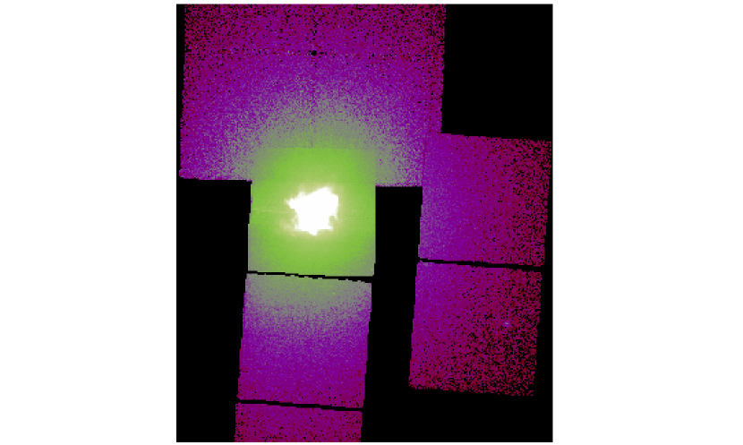
Figure 1: Summed Chandra observations in the range 0.4-2.1 keV showing the bright nebula and faint halo. Data have been smoothed with a Gaussian of $9^{\prime\prime}$ FWHM. Some ACIS chips are only partly shown in this figure. Reading left to right, top to bottom (like a book), the chips are: I3, I1, I2, I0, S3, I3, S2, I2, S1.

Figure 1 shows the sum of these 3 observations in the energy range 0.4–2.1 keV. To show the inner nebula, one of the 4 ks observations of the bright Crab has been normalized and added to fill the hole left by telemetry exclusion. Cosmic-ray background has been subtracted and time variation of chip sensitivity has been included. The ACIS charge-transfer streak has been subtracted from chip S3, on which the Crab is imaged, and from the 2 I chips north of and overlapping the field of S3. In order to show detail at the center, some chips are only partially shown in this figure. Since calibration of some chips is more extensive than for others, chip IDs are listed.

There is appreciable structure at the outer boundary of the PWN. The faintest features visible are $2.5^{\prime}$ from the center of the nebula and these have surface brightness a factor of 200 less than that where the PWN is brightest. The halo data extend from this radius, which is inside the optical nebula, to a radial distance of $18^{\prime}$. In this span, the halo brightness decreases a factor of 100. Coverage of the halo is 100% at radial distances from $2.5^{\prime}$ to $4^{\prime}$, is greater than 60% out to $10^{\prime}$, and falls to 25% at $18^{\prime}$.

Figure 2 shows measured surface brightness extending from the center of the Crab to the outermost chip boundaries. Data from the central, northern, and western chips indicate a halo with intensity independent of azimuth. The 2 southern chips, S2, and S1, show greater surface brightness. This is, at least partially, a calibration problem. Excluding these 2 chips, the halo is symmetric about the point: RA = 05 34 31.3, Dec = 22 01 03, located $14^{\prime\prime}$ northwest of the pulsar and within the bright X-ray torus.

Figure 3 shows the Chandra-measured surface brightness compared to that measured by ROSAT (Predehl and Schmitt 1995). The energy range of both observations is $\approx$ 0.4-2.1 keV but the ROSAT sensitivity from 1.5-2.1 keV is considerably less than that of Chandra. To obtain the strength of the Chandra dust halo, the Chandra mirror scattering (dashed line) must be subtracted from the observed brightness (solid line). Note that the Chandra measurement, even before this correction, falls below the ROSAT observation. The mirror scattering was taken from an observation of Her X-1 combined with ground calibration as summarized by Gaetz (2004). The strength of the Chandra dust halo integrated from $2.5^{\prime}$ to $18^{\prime}$ and interpolated from $0^{\prime}$ to $2.5^{\prime}$, is 0.047 that of the Crab Nebula. (The interpolation from $0^{\prime}$ to $2.5^{\prime}$ accounts for .010 of this.) The ROSAT-measured scattered fraction from $0^{\prime}$ to $30^{\prime}$ is 0.080 (Predehl & Schmitt 1995). An extension of our Figure 3 curve to $30^{\prime}$ would increase the Chandra-measured fraction to $0.048\pm 0.008$. Uncertainties comprise measure of surface brightness, measure of total crab count rate, extrapolation to small radii, background subtraction, and an assumed 20% error in the mirror scattering.

We note that we have used data taken N and E of the Crab and we have assumed that this is valid for all azimuths. We have not included data from the 2 southern ACIS chips because the discontinuity at the chip boundary indicates a normalization problem. If we assume that the higher surface brightness indicated by these chips (S1,S2) is real, and that this higher brightness applies to a sector extending $90^{\circ}$ in azimuth, the Chandra-observed scattered fraction to $30^{\prime}$ would increase to 0.051, which is within our margin of error. Since the ROSAT and Chandra detectors have different spectral sensitivities, even though the energy range covered here is about the same as that of ROSAT, the fraction of counts in the halo is not expected to be the same. Using the known spectrum of the Crab and the halo spectra given here at the end of Section 4, we expect the relative strength of the dust halo measured with Chandra to be 82% of that measured with ROSAT (because the ROSAT detector is relatively more sensitive at low energies). We observe a halo strength $60\%\pm 10\%$ that of ROSAT so conclude that the ROSAT result is too high.

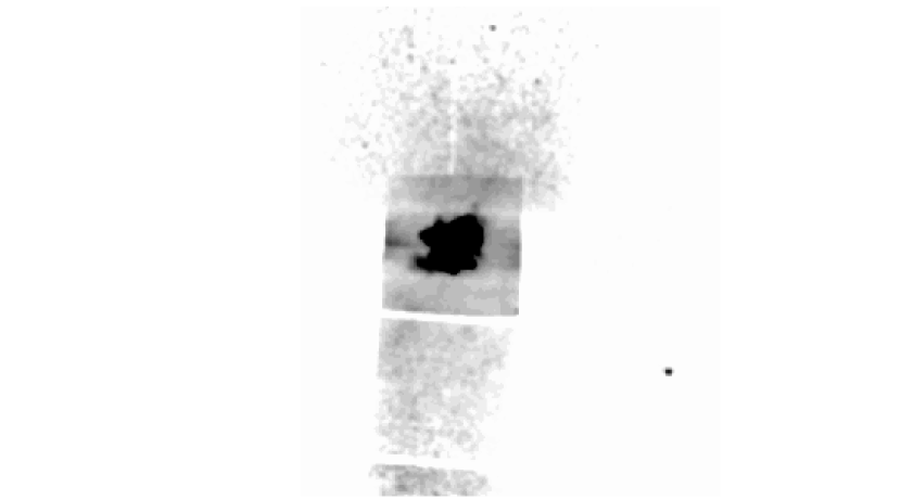
Figure 4: Regions of above average surface brightness. Generation of this figure is described in Section 2. Horizontal bands in the central chip, S3, show imperfect subtraction of the charge-transfer streak. The brightness of the halo in the southernmost chip, S1, and the weakness of the halo in the 2 western chips could indicate that the relative chip normalization is not quite correct.

Figure 4 was made to illustrate fluctuations in halo surface brightness. The 0.2-2.1 keV data shown in Figure 1 was first smoothed to make map $M$. Then a function $F(r)$, with about the same radial dependence of surface brightness was subtracted. $F(r)=constant[1+(r/240)^{2}]^{1.05}$, where $r$ is distance from the scattering center in ACIS pixels. The figure shows the quantity $(M-F)/F$ and one can see regions N and S of the Crab which are $\sim 10\%$ brighter than average. Note that since the average decrease of brightness with radial distance has been removed from Figure 4, any extended above-average component also is decreasing with radial distance, contrary to appearance in Figure 4. We interpret the significant features in Figure 4 as possible structure in the dust distribution and/or variations in column density of absorbing gas in the line-of-sight. The $1^{\prime}-2^{\prime}$ feature $5^{\prime}$ SSE of the Crab center is discussed further in section 4. Note that any gradual radial variation in brightness implied by Figure 4 may be an artifact due to the form assumed for the subtracted function, F(r). Apparent azimuthal variation should be real. Because we are seeing variations of a few percent, chip-to-chip calibration uncertainties show. A variable contamination layer on the instrument window is also a cause for concern. This layer, however, is thicker at the edges of the window and, if present, should produce a recognizable effect. This is not seen.

The halo spectrum contains no strong sharp features which might indicate thermal emission from a shock. Reasonable fits are obtained using the sum of power law and thermal bremsstrahlung (used as an arbitrary continuum) components. The signal is comprised of dust-scattered halo, mirror scattering, and background, which is negligible except for high energies at large angles.

3 Upper limits to outer shell

To be detectable, X-rays from any shock-heated material must be visible over the dust-scattered halo. Since diffuse uniform emission is more difficult to detect than bright knots, we consider a hypothetical diffuse shell which represents the most massive allowed shell possible. The limiting surface brightness is taken as 0.1 of the observed dust halo.

Upper limits depend on radius, $R$, of the assumed shell and were calculated assuming a spherical shell of thickness $0.15R$ centered on the pulsar and filled with material of uniform density, $n$ cm^-3. Using the dashed curve of Figure 5 (0.1 of the observed halo) as the surface brightness of the unseen shell, limits on several quantities are calculated and shown in Figure 6. The upper limit to $n$ is 4 just inside the optical nebula and drops to 0.15 at $R=18^{\prime}$. If the surrounding ISM is uniform, since $n$ is swept-up material, the ISM density, $n_{0}$ would be 0.4 of these values. The limit on the X-ray luminosity, $L_{x}$, of any shell is $\approx 10^{34}$ ergs s^-1 and almost independent of $R$. Uncertainty of the gas temperature leads to an uncertainty of $\pm 25\%$ in $n$ and $\pm 40\%$ in $L_{x}$. The calculation of $n$ and $L_{x}$ is straightforward. A model is necessary to derive paremeters of the explosion. It is customary to estimate the energy of the shock, $E_{\circ}$, using a simple blast-wave model (Cox, 1972). For a uniform ISM, $E_{\circ}/n_{0}=1.6\times 10^{-6}R^{5}t^{-2}$, where the units of $E_{\circ}$ are $10^{51}$ ergs, $R$ is in parsecs and the age, $t$ is in $10^{4}$ years or, in this case, $t=.095$. Upper limits for $E_{\circ}$ are shown in Figure 6.

The crosses in Figure 5 show measured surface brightness of selected “bright spots”. These illustrate that the limit of bright knot detectability is about 0.1 the brightness of the dust halo. All are consistent with statistical fluctuations except for the point at $R=2.6^{\prime}$ which is a small cloud of emission within the N boundary of the optical nebula. At $R=12^{\prime}$ the bright lumps represents a knot size of $\sim 1$ pc and a lump luminosity of $3\times 10^{28}$ ergs. Assuming we would notice 10 such lumps in a $30^{\circ}$ arc, this would imply 300 lumps in the shell, a total $L_{x}=10^{31}$ ergs and total mass of $2\times 10^{-2}$ M_⊙. As expected, these limits are far below the limits calculated for a diffuse uniform shell.

The circles in Figure 5 show surface brightness of shells observed by Chandra in other remnants (Seward et al 2004). Most remnants have an irregular outer shell which defines the boundary and brighter patches at a lesser radius. In this figure, we have shown brightness and radial position for both the brightest part of the shell and the emission observed over most of the outer boundary. Radii have been corrected to show the size at 2 kpc distance. Although surface brightness does not depend on distance, corrections have been made for differing absorption measured in the ISM. The remnants Kes 75 and SNR 0540-69.3 have bright central PWN very similar to that of the Crab and, in this respect, are the most Crab-like remnants known.

We searched, without success, for thermal emission inside the optical nebula. There are many faint features at the edge of the PWN. All have soft power-law spectra and are best interpreted as part of the PWN. The density of any unseen thermal X-ray-emitting diffuse material must be $<4$ and the mass $<0.2M_{\odot}$. The limits on lumpy material are appreciably less.

4 Dust scattering

Although no emission from an outer shell has been recognized, there is substantial extended emission observed due to scattering from dust in the interstellar medium (ISM) and mirror scattering in the Chandra HRMA. As we will show, below $\approx$ 2.5 keV scattering by dust grains dominates the extended emission; above $\approx$ 3 keV mirror scattering becomes the primary contribution.

X-ray scattering by ISM grains, first described by Overbeck (1965), has been observed by instruments on Einstein (Mauche & Gorenstein, 1986), ROSAT (Predehl & Schmitt, 1995), Chandra (Clark, 2004, Smith, Edgar, & Shafer, 2002), and XMM (Vaughan et al. 2004). Theoretical studies have been done by Mathis & Lee (1991), Predehl & Klose (1996), and Smith & Dwek (1998).

The total scattering cross section in the Rayleigh-Gans (RG) approximation illustrates the dependence on X-ray energy and grain characteristics. It is applicable when $E>2$ keV and is

$$\sigma(E,a)=6.3\times 10^{-7}\Big{(}{{2Z}\over{M}}\Big{)}^{2}\Big{(}{{\rho}\over{3\hbox{g\,cm}^{-3}}}\Big{)}^{2}a_{\mu\rm m}^{4}E_{\rm keV}^{-2}{\rm cm}^{2}$$ (1)

where $a$ is the grain radius, $Z$ is the mean atomic charge, $M$ the mean atomic weight (in amu), $\rho$ the mass density, and $E$ the X-ray energy in keV (Mathis & Lee 1991). Eq. 1 implies that the overall scattering halo will tend to be brighter at lower energies, from the $E^{-2}$ term [note error in Mathis & Lee (1991) showing this as $E^{2}$]. Figure 7 plots the total scattering fraction between $120-1000^{\prime\prime}$, the range observed here, assuming a column density of N${}_{\rm H}=10^{21}$ cm^-2. Three different dust models, Mathis, Rumpl, & Nordsieck (1977) (MRN), Weingartner & Draine (2001) (WD01; using $R_{V}=3.1$ and $b_{C}=6\times 10^{-5}$), and Zubko, Dwek & Arendt (2004) (ZDA04; using the BARE-GR-B parameters) are shown using both the exact Mie solution for scattering from a sphere and the approximate RG solution. In all cases the RG approximation clearly begins to break down below 1.5 keV, although the scattering is generally larger at lower energies. The ZDA04 model, which has relatively fewer large grains than the MRN and WD1 models, gives the best fits of the three to our data (see Figure 8).

The analysis to be described used only data from the 4 I chips of the 14 April 2002 observation (obsid 2798). There was a charge-transfer streak in chip I0 due to part of the Crab PWN at the edge of the chip. The charge transfer streak was therefore subtracted from the 2 chips closest to the Crab. For each energy interval, the counts were projected along the transfer axis and summed. 0.013 of this sum was then subtracted from each element of the image.

At almost any energy, extracting an X-ray scattering halo from the observations first requires that the Chandra PSF be subtracted. As described by Smith et al. (2002), ray-trace models of the Chandra PSF (such as ChaRT) significantly underestimate the scattering at angles beyond $1^{\prime}$. Therefore we followed Smith et al. (2002) and used an on-axis Her X-1 observation (obsid 3662) as our PSF calibrator. This has the obvious limitation that this observation was done on-axis, while our Crab observation was done with the Crab $\sim 10^{\prime}$ off-axis. We believe that this is reasonable because at 4 keV, where dust scattering is minimal, the observed Crab profile matches the Her X-1 profile. We note, however, that while this match is suggestive it does not guarantee that there are no differences in the PSF at lower energies.

Unlike most halo studies, the Crab nebula is not a point source but rather an extended nebula $\sim 1^{\prime}$ in radius. We calculated the radial profile assuming it was centered at 05:34:31.3, 22:01:03 (J2000), which is both roughly central and near the peak of the nebular emission. This is not the location of the Crab pulsar, however, which itself emits only 5% of the X-ray emission. The effect of source extent is relatively minor except at scattering angles comparable to the size of the source. With the assumption that the source is circular with uniform surface brightness, the effect can easily be calculated by integrating the point-source scattering intensity over the surface:

$$I(\theta,\phi)=2\int_{\theta-\phi}^{\theta+\phi}d\psi\psi\arccos((\theta^{2}-\phi^{2}+\psi^{2})/(2\theta\psi))I(\psi)$$ (2)

where $\phi$ is the source radius on the sky and $I(\theta)$ is the scattered halo at angle $\theta$. This equation holds for $\theta>\phi$; in most cases, when $\theta<\phi$ the source brightness itself will swamp the scattered halo.

We extracted the radial profile of the Crab Nebula in energy slices between 0.5-4 keV. Between 0.5-1.0 keV, we used an energy width of 0.1 keV (approximately equivalent to the energy resolution of the ACIS CCDs), and between 1.0-4.0 keV we used a width of 0.2 keV. We modeled the Crab as a uniform circle of radius $1^{\prime}$, and fit it using various dust models using Eq. 2 and either the Mie solution (for energies below 1.5 keV) or the RG approximation (above 1.5 keV). Sample results at 1 and 2 keV, assuming the dust has an MRN-type size distribution and is smoothly distributed between the Crab and the Sun are shown in Figure 8.

As Figure 8 shows, by 2 keV the observed radial profile is strongly influenced by the power-law shape of the PSF; at 1 keV, the shape of the observed profile shows dust scattering is dominant. The 1 keV X-ray surface brightness is poorly fit by the MRN model. Changing the assumed dust model to a WD01 or ZDA04 model does not significantly improve the fits.

If the dust is assumed to be smoothly distributed along the line of sight, the choice of a dust grain model leaves only the total dust column density as a free parameter; this can easily be converted to a gas column density using the dust model parameters. In Figure 9 we show the best-fit hydrogen column density for the three different dust grain models as a function of energy. Since the energy dependence of the halo emission has already been taken into account in the model fits, any variation with energy indicates the model does not completely describe the data. Figure 9 shows that the best-fit column density from the halo data is significantly lower than the best-fit column density derived from fitting the X-ray spectrum, $N_{H}\approx 3.5\times 10^{21}$ atoms cm^-2. This result disagrees with that of Predehl & Schmitt (1995) but is consistent with our observation of less halo emission than they saw with ROSAT.

Regarding the variations seen in Figure 9, an examination of the individual halo fits showed that this simple ”smoothly distributed dust” model fit best at energies between 1.5-2.5 keV. At higher energies, we believe that errors in the mirror scattering model dominate the fits. At lower energies, it seems likely that the one-component model is too simple, as described below. We also note that the error bars in Figure 9 are purely statistical, and do not include the known but difficult-to-estimate systematic errors such as the energy dependence of the Chandra mirror point-spread function.

To improve the fits, we experimented with more complex models, with two halo components: a “smooth” component plus a single cloud of dust between the Sun and the Crab. In this case, we find reasonable fits, although the column density varies a bit with energy. We find that the planar dust to be very near, with a column density of $\sim 4-5\times 10^{20}$ cm^-2, while the smooth dust has a column density of $\sim 8-9\times 10^{20}$ cm^-2 for MRN-type dust. If instead we use a ZDA04 dust model (specifically their BARE-GR-B model), as shown in Figures 10 and 11, we get significantly improved fits over a MRN-type distribution. Again, this column density is lower than normally used for the Crab, and is affected by the dust size distribution chosen.

Interestingly, the Local Bubble (LB) radius is, on average, $\sim 100$ pc distant (Cox & Reynolds, 1987). Assuming an “average” IS density of 1 cm^-3 existed before the LB was swept out implies the edge would have a column density $\sim 3\times 10^{20}$ cm^-2. Observations of the LB edge by Lallement et al. (2003) show that the edge in the direction of the Crab is at $\sim 200$ pc, with a column density greater than $10^{20}$ cm^-2.

Although plausible, we cannot conclude that this excess at large angles is due to the LB edge. It could also be caused by additional small dust particles that are not in the model, or even due to a missing mirror scattering term. In addition, at these large angles the data is from the outer two CCDs. Therefore there is no blurring correction from the bright edge of the nebula, although calibration differences between the various chips could contribute to the excess as well.

In sum, our primary results concerning dust are:

• The ZDA04 model seems to best fit the radial dependence of surface brightness.

• There appears to be less dust along the line of sight to the Crab than would be predicted from the best-fit N_H value for the Crab spectrum, although this may depend on the dust model used.

• There is evidence for a nearby plane or cloud of dust with a moderate column density.

Figure 12 shows the spectrum of the halo $6.5^{\prime}$ SSE of the scattering center. The mirror scattering is approximated by a broken power law with indices 1.1 and 2.8 and a break at 4.6 keV. All events with energies above 2.5 keV are assumed to be from the mirror. The dust contribution below 2.5 keV was approximated and characterized by a continuum. Of the several simple models readily available, a bremsstrahlung spectrum gave the best fit with about the right value for $N_{H}$. No emission mechanism is implied. The residuals to halo spectra typically show a multiple peaked structure between 0.8 and 2 keV. This structure, which varies from place to place and is about 5% of the signal at most locations, is not understood. Adding models with line emission does not produce reasonable fits. Some of the structure may be an artifact of the detector. For example, some spectra contain a line feature at 1.5 keV which probably comes from an Al coating on the detector window. In any case, the “temperature” of the bremsstrahlung continuum characterizes the dust-scattered spectrum. Some results at varying distances are: $4.5^{\prime}$, 0.48 keV; $6.5^{\prime}$, 0.37 keV; $8.5^{\prime}$, 0.32 keV; $15^{\prime}$, 0.23 keV. As expected, the scattered spectrum is softer as scattering angle increases.

5 Nearby sources

The Chandra mirror is well suited for the detection of point sources embedded in diffuse emission. There are 19 serendipitous sources visible to the eye in the field shown in Figure 1. Because of smoothing, compression, and color map, only one is visible (barely) at the western edge of Figure 1 but shows clearly in Figure 4. The closest source to the Crab Nebula is at RA = 05 34 45.91, Dec = 22 00 11.6 (2000). This is $3.3^{\prime}$ from the pulsar and on the eastern boundary of the optical nebula. Strengths range from 1 to 12 counts ks^-1 and none fall clearly within the projection of the optical nebula.

6 Discussion/Conclusions

There is no indication in our observation of X-ray emission from an outer shell. The shell predicted assuming the expected type II SN progenitor has $\approx 4M_{\odot}$ and is moving at $\approx 5000$ km s^-1. If the “usual” blast wave analysis of Section 3 is done, we conclude that this shell does not exist. At a radius of $R=10^{\prime}$ a uniform shell containing $\approx 2M_{\odot}$ and indicating an explosion energy of $10^{50}$ ergs is possible but highly unlikely. All other remnants which have prominent outer shells are irregular. If the Crab outer shell were similarly clumpy, limits on emission, would be considerably lower than the limits used here. Our upper limits for emission are already a factor of 100 - 1000 below that observed from shells around SNR 0540-69.3 and Kes 75 which have small bright PWNe similar to the Crab. Even the weak plerionic remnant G21.5-0.9, with central pulsar and surrounding PWN ($70\times$ less luminous than the Crab) has 2 shell-like features which, as shown in Figure 5, are still $\sim$ 10 times brighter than our limit.

At radii $>10^{\prime}$, a larger mass and energy are possible and our coverage becomes sparse. ROSAT and Einstein observed out to $30^{\prime}$ with 100% coverage and found no shell-like emission: so we know there is no bright shell just outside the Chandra field of view. A faint shell is possible.

The freely-expanding ejecta proposed by Sankrit and Hester (1997) and by Sollerman et al (2000) consists of photoionized $10^{4}-10^{5}$ K material and is too cool to be detected by Chandra. Shock-heated material, however, will be present where this fast moving ejecta plows into the pre-supernova environment. This would be detectable by Chandra if the density of the shocked material were high enough. The Sollerman et al shell density varies as $R^{-3}$; our upper limit varies as $R^{-2}$. Assuming a shock structure similar to that given by Chevalier (1982, Figure 2), the reverse shock in the ejecta should have a density 4 $\times$ that in the unshocked material. For the Sollerman et al minimum-mass model, this is above our limit at $R<6^{\prime}$. The shock in the presupernova ISM, assuming a similar density jump, would be below our limit at all $R<18^{\prime}$ if $n_{0}<.02$.

In conclusion, with reasonable assumptions about non-uniform distribution and density, we find no evidence for the shell expected from an $8-13M_{\odot}$ SN in the region $2^{\prime}<R<\approx 8^{\prime}$, where the velocity of freely-expanding material ranges from $\approx 1200$ to $\approx 4800$ km s^-1. We cannot exclude models postulating several $M_{\odot}$ of ejecta with temperature $10^{4}-10^{5}$ K if the circumstellar density is very low ($\sim.01$) and rather uniform. We note that quantitave comparison with these models is very uncertain

Although our X-ray upper limit is an order of magnitude lower than past work, we cannot firmly exclude a $10^{51}$ erg explosion of a $8-13M_{odot}$ progenitor. Certainly the range of possible circumstances is narrowing. Any hidden mass is almost invisible. We note that 3C 58 (Slane et al 2004) and G054.1-0.3 (Lu et al 2002) have central pulsars and PWN but have weak (or absent) X-ray emitting shells. Although both only $1.5\times 10^{-3}$ as luminous as the Crab, these, together with the Crab, may form a class of gravitational-collapse SNe with unusual progenitors.

This work was supported by Chandra Grants GO2-3087X and GO4-5059X. We thank Rob Fesen for a critical reading of the manuscript, for several important references, and for showing enthusiasm over a non-detection observation.

7 References

Bowyer, S., Byram, E., Chubb, T., & Friedman, H., 1964, Science 146, 912

Brinkman, W., Aschenbach, B. & Langmeier, A., 1985, Nature 313, 662

Clark, G.W. 2004, ApJ 610, 956

Cox, D.P., & Reynolds, R.J. 1987, ARA&A, 25, 303

Chevalier, R.A., 1977, in Supernovae, edited by D. N. Schramm (Reidel, Dordrecht), p53.

Chevalier, R.A., 1982, ApJ 258, 790

Chevalier, R.A., 1985, in The Crab Nebula and Related Supernova Remnants, edited by M. C. Kafatos and R. B. C. Henry (Cambridge University Press, Cambridge), p. 63.

Fesen, R.A., Shull, J.M., & Hurford, A.P., 1997, AJ 113, 354

Frail, D.A., Kassim, N.E., Cornwell, T.J., & Goss, W.M., 1995, ApJ 454, L129

Gaetz, T.J., 2004, Chandra X-ray Center memorandum, 23 June 2004

Harnden Jr., F.R. & Seward, F.D., 1984, ApJ 283, 279

Hester, J.J., et al., 1995, ApJ 448, 240

Hester, J.J., et al., 2002, ApJ 577, L49

Hwang, U., Petre, R., Holt, S.S., & Szymkowiak, A.E., 2001, ApJ 560, 742

Lallement, R., Welsh, B.Y., Vergely, J.L., Crifo, F., & Sfeir, D., 2003, A&A 411, 447

Lawrence, S., MacAlpine, G., Uomoto, A., Woodgate, B., Brown, L., Oliversen, R., Lowenthal, J., & Liu, C. 1995, AJ 109, 2635

Lu, F.J., Wang, Q.D.,Aschenbach, B., Durouchoux, P., & Song, L.M., 2002, ApJ 568, L49

Mathis, J.S., Rumpl, W. & Nordsieck, K.H. 1977, ApJ 217, 425

Mathis, J.S. & Lee, C.W. 1991, ApJ 376, 490

Mauche, C.W. & Gorenstein, P., 1986, ApJ 302, 371

Mauche, C.W. & Gorenstein, P., 1989, ApJ 336, 843

Murdin, P. & Clark, D.H. 1981, Nature 294, 543.

Murdin, P., 1994, MNRAS 269, 89

Overbeck, J. W. 1965, ApJ 141, 864

Palmieri, T.M., Seward, F.D., Toor, A., & Van Flandern, T.C., 1975, ApJ 202, 494

Predehl, P. & Schmitt, J.H.M.M., 1995, A&A 293, 889

Predehl, P., & Klose, S., 1996, A&A 306, 283

Sankrit, R. & Hester, J. 1997, ApJ 491, 796

Seward, F.D. & Harnden, F.R., 1994, ApJ 421, 581

Seward, F., Slane, P., Smith, R., Gaetz, T., Lee, J.J., Koo, B.C., 2004, http://snrcat.cfa.harvard.edu

Slane, P.O., Helfand, D.J., van der Swaluw, E. & Murray, S.S., 2004, ApJ 616, 403

Smith, R.K. & Dwek, E. 1998, ApJ 503, 831

Smith, R.K., Edgar, R.J., & Shafer, R.A., 2002, ApJ 581, 562

Toor, A., Palmieri, T.M., & Seward, F.D., 1976, ApJ 207, 96

Trimble, V., 1968, AJ 73, 535

Trimble, V. & Woltjer, L., 1971, ApJ 163, L97

Vaughan, S., et al. 2004, ApJL 603, L5

Wallace, B.J., Landecker, T.L., Kalberla, P.M.W., & Taylor, A.R., 1999, ApJS 124, 181

Weingartner, J.C. & Draine, B.T., 2001, ApJ, 548, 296

Weisskopf, M.W. et al., 2000, ApJ 536, L81

Zubko, V, Dwek, E. & Arendt, R. 2004, ApJS 152, 211

Figure 2: Measured surface brightness in 4 directions. Vertical lines show edges of the ACIS chips. Data closer than $4^{\prime}$ are all from chip S3; beyond $4^{\prime}$, data are from 7 different chips

Figure 3: Dust halo surface brightness measured by Chandra and ROSAT. Mirror scattering has been subtracted from the ROSAT data but not from the Chandra data.

Figure 5: Chandra-measured surface brightness around the Crab. The dashed curve is 0.1 of the observed halo and is our threshold of detection. Crosses show some of the larger fluctuations in the brightness pattern and illustrate that the dashed curve is a reasonable detection threshold. The cross at $2.5^{\prime}$ is a real feature, visible in Figure 4; others are statistical fluctuations (with number-of-counts uncertainties). Circles indicate approximate radii and brightness of other remnant shells if viewed from 2 kpc distance.

Figure 6: Upper limits calculated for a uniform shell with brightness at the threshold of detection.

Figure 7: The total scattering fraction as a function of energy between $120-1000^{\prime\prime}$ using three dust models and both the Mie solution and the RG approximation. Although there is a significant difference between the models at low energies in the RG approximation, the difference is much less when the Mie solution is used.

Figure 8: Crab radial profiles at 1 ($\times$) and 2 ($\Box$) keV, fit with a smoothly-distributed MRN, WD01, and ZDA04 dust models. The 1 keV fit used the Mie solution and the the 2 keV fit the RG approximation. At 1 keV, the ZDA04 model is the best fit, although still poor; at 2 keV, the profile is dominated by mirror scattering with a weak dust halo in all three cases.

Figure 9: The best-fit values of N_H for the MRN, WD01 (using their $R_{V}=3.1$, $Ab_{C}=6.0$ model), and ZDA04 (using their BARE-GR-B model) assuming a smooth spatial dust distribution. Error bars show the statistical error only. However, most of these fits have $2<\chi^{2}<10$, implying that the errors are not purely statistical.

Figure 10: Crab radial profiles at 1 and 2 keV, fit with a two-component MRN model with both smoothly-distributed plus a single dust cloud. Data errors are approximately the size of the symbols. The best-fit column densities are $8\times 10^{20}$ cm^-2 and $4\times 10^{20}$ cm^-2 respectively for the 1 keV profile, and $9\times 10^{20}$ cm^-2, $5\times 10^{20}$ cm^-2 at 2 keV. At both energies, the fit puts the dust cloud very near the Sun.

Figure 11: Same as Figure 10, using a ZDA04 BARE-GR-B-type model. In this case the best-fit column densities are slightly larger, $1.3\times 10^{21}$ cm^-2 and $4\times 10^{20}$ cm^-2 at 1 keV, and $2\times 10^{21}$, $2\times 10^{20}$ cm^-2 at 2 keV. In this case, the best-fit cloud position is at 0.04 of the distance to the Crab, or $\sim 100$ pc.

Figure 12: X-ray spectrum of the halo 6^′ from the center of the nebula. The fit is the sum of a broken power law and a thermal bremsstrahlung continuum

Table 1: Chandra observations

observation number	date	live time	ACIS chips
500174/1997	14 Mar 2001	3972	S3
500248/2798	14 Apr 2002	19981	I0,I1,I2,I3
500432/4607	27 Jan 2004	37250	S3
500432/4607	27 Jan 2004	38090	I2,I3,S1,S2