Photometric entropy of stellar populations and related diagnostic tools

Abstract

We discuss, from a statistical point of view, some leading issues that deal with the study of stellar populations in fully or partially unresolved aggregates, like globular clusters and distant galaxies. A confident assessment of the effective number and luminosity of stellar contributors can provide, in this regard, a very useful interpretative tool to properly assess the observational bias coming from crowding conditions or surface brightness fluctuations. These arguments have led us to introduce a new concept of “photometric entropy” of a stellar population, whose impact on different astrophysical aspects of cluster diagnostic has been reviewed here.

INAF - Osservatorio Astronomico di Bologna, Via Ranzani 1 - 40127 Bologna (Italy)

1. Introduction

Galaxy surface brightness fluctuations and crowding effects in nearby star clusters are two related and well recognized features one has to deal with when observing partially or fully unresolved stellar systems. The latter effect turns out to be a severe problem, for instance, when probing the innermost regions of globular clusters in our own galaxy, and more generally in all those situations when the stellar plot consists in fact of blended point sources, at different spatial scales.

On the other hand, to a more detailed analysis, even the smooth surface brightness of distant galaxies actually is found to display some intrinsic “clumpiness”, and this special property can be usefully exploited to derive information on their fully blended composing stellar populations, as first shown by Tonry & Schneider (1988) and Tonry (1991).

In this contribution, we would like to further extend the analysis of these two important issues, that deeply relates to overall characteristics of stellar aggregates and the way the latter are sampled by the observations. In particular, we will show that both effects are in fact a consequence of the same property of finiteness and discreteness of the composing stellar populations, and this will lead to a unified and more general definition of “photometric entropy” of a stellar population, a relevant concept whose impact on different astrophysical aspects of cluster diagnostic we want to review here.

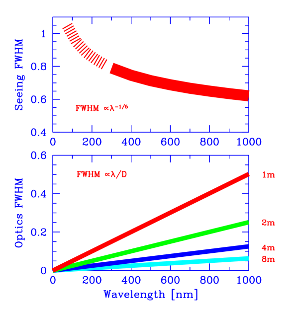
Figure 1.: Upper panel - The expected trend of seeing variation with varying wavelength, after Wynne (1999). From empirical estimates and theoretical arguments, the FWHM of the seeing disk is found to scale approximately as FWHM${}_{\rm seeing}\propto\lambda^{-1/5}$. Lower panel - Telescope resolving power with varying the aperture diameter, $D$, (right labels, in meters). As predicted by the classical Airy diffraction pattern, FWHM${}_{\rm Airy}\propto\lambda/D$. Contrary to seeing, optics performance degrades when moving to long-wavelength photometric bands.

2. Observational constraints

Our attempt to single out any “clean” information of a cluster stellar population crucially relies on how confidently we approach the ideal observing conditions, that is those allowing us to fully resolve any star member in the system. Apart from the obvious constraint due to the physical distance of our target and its apparent size, there are at least three relevant external mechanisms that play a role to bias our results when carrying out imagery (or spectroscopy) of a stellar aggregate.

• Photon noise directly relates to the signal-to-noise ratio ($S/N$) of our observations, the latter being constrained both by telescope size and, in case of ground-based observations, by sky brightness. In particular, we know that, for faint sources, $S/N$ mainly scales with the telescope aperture ($D$), the exposure time ($t_{\rm exp}$), and the sky surface brightness (ssb), in magnitudes per square arcsec, such as

  $$S/N\propto(1/D)\times(1/\sqrt{t_{\rm exp}})\times 10^{0.2\,{\rm ssb}}.$$ (1)

• Telescope resolving power is also an issue. It can be quantified by the full width at half maximum (FWHM) of the instrumental diffraction pattern (the “Airy disk”), that is a measure of the minimum physical “spot” of a star on our imagery detector (or spectrograph slit), if we could observe outside the atmosphere. The Airy disk depends itself on $D$, but scales with the observing wavelength, as well, so that

  $${\rm FWHM}_{\rm Airy}\simeq{\lambda\over D}.$$ (2)

• Finally, seeing conditions, in case of ground-based observations, drastically depend on sky clarity and, opposite to the telescope resolving power, improve in general at longer wavelength, mainly due to a better spatial coherence of the atmosphere convection layers with increasing $\lambda$. Theoretical arguments and empirical estimates (Wynne 1999) indicate that FWHM of the seeing disk scales as

  $${\rm FWHM}_{\rm seeing}\propto\lambda^{-1/5}.$$ (3)

While, to some extent, we could improve $S/N$ of our observations (and “see more clearly”) by arbitrarily increasing exposure time (although with some non-negligible technical limits due to detector saturation, electronic noise etc.), the other two effects are much more difficult (and expensive) to be optimized, as one would need either a bigger telescope and/or space-based observations to fully remove any atmosphere contamination. The combined action of telescope resolving power and seeing provides therefore the observational kernel that constrains our ability to master the crowding conditions and fully resolve the stellar population (see Fig. 1).

For example, for the typical case of a $\sim 50$ pc globular cluster around the Andromeda galaxy (about 0.7 Mpc away) a mean angular separation of the order of $0.04\hbox{${}^{\prime\prime}$}$ should be expected among the $\sim 10^{5}$ star members of the cluster. Such an equivalent resolving power would certainly not be achieved by means of any seeing-limited conventional telescope on the ground, rather demanding at least a 2.5 m orbiting telescope (as it is actually the case for the Hubble Space Telescope, indeed!).

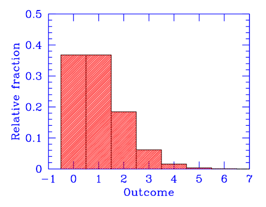
Figure 2.: The Poissonian distribution of the $N_{\rm tot}$ star cells in our “fair statistical representation” of a stellar population. In average, each cell contains one star, according to the Poisson formula, $p(x)={{e^{-1}}/x!}$. As a consequence, after repeated trials, the total number of stars, $N_{\rm tot}$, is expected to fluctuate by $\sigma(N_{\rm tot})=\sqrt{N_{\rm tot}}$.

3. Effective numbers of luminous contributors and photometric entropy

Although within the limits of the instrumental performance and seeing influence (both being, however, quantitatively assessed and, at least partially, recovered), one can still take advantage of the overall statistical properties of a stellar sample and gain valuable information, in any case, of its unresolved component.

In this regard, photometric entropy adds an important tool to our analysis. As we will see in a moment, its definition has much to do with the concept of “effective number” of stellar contributors to the integrated luminosity of a stellar population. This quantity has been first assessed in a series of previous papers (Buzzoni 1989, 1993), providing the reference framework for further theoretical investigations (Cerviño, Luridiana & Castander 2000; Cerviño et al. 2001, 2002; Cerviño & Luridiana 2004). We will just sketch here some of the leading issues of the theory and the main relationships among the relevant statistical quantities involved in our analysis.

First of all, it is important to define operationally what we call a “fair statistical representation” of a stellar population. Ideally, we could assume to have a number $N_{\rm tot}$ of cells, each to host, in average, one star to be supplied to the system through a stochastic process of Poissonian nature. After completion of $N_{\rm tot}$ iterations, each cell will display a star distribution ($n_{j}$) like in Fig. 2, and the whole system will contain, in average, $\sum_{j=1}^{N_{\rm tot}}n_{j}=N_{\rm tot}$ stars.

Due to the Poissonian distribution of $n_{j}$, however, in repeated statistical realizations of the population, the total number of stars will fluctuate by $\sigma(N_{\rm tot})=\sqrt{N_{\rm tot}}$.

If we assume, to a first analysis, that all stars have the same luminosity $\ell$, then the expected relative fluctuation of the global luminosity ($L_{\rm tot}$) of the sample is:

$${{\sigma(L_{\rm tot})}\over{L_{\rm tot}}}={{\sqrt{\sum_{j}n_{j}^{2}\ell^{2}}}\over{\sum_{j}n_{j}\ell}}={{\ell\sqrt{N_{\rm tot}}}\over{\ell N_{\rm tot}}}=1/\sqrt{N_{\rm tot}}.$$ (4)

More likely, if $\ell_{j}$ is not a constant, and distributes according to a given luminosity function, then we could still retain eq. (4), just replacing $N_{\rm tot}$ in the r.h. side of the formula with a more general quantity $N_{\rm eff}$. The value of $N_{\rm eff}$ can be regarded as an “effective” number of stellar contributors in the population; it could be demonstrated that, always,

$$N_{\rm eff}\leq N_{\rm tot}.$$ (5)

Quite importantly, as the luminosity distribution of stars changes with wavelength, one has to expect that

$$N_{\rm eff}=N_{\rm eff}(\lambda).$$ (6)

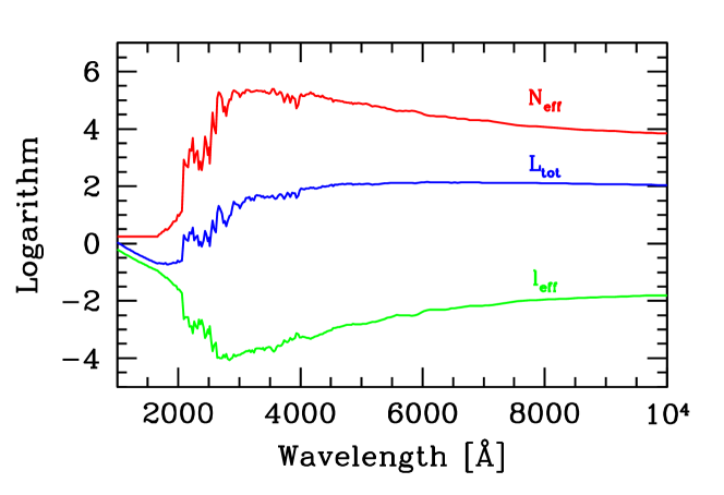
Figure 3.: Logarithm of effective luminosity ($\ell_{\rm eff}$) and star number ($N_{\rm eff}$) for a 15 Gyr SSP of solar metallicity and Salpeter IMF, from Buzzoni (1993). Both quantities relates to the global luminosity ($L_{\rm tot}$) of the stellar population through eq. (10). The model has been rescaled to a total SSP bolometric luminosity of $10^{7}$ L_⊙.

On a similar argument, the relative variance of the luminosity ($L_{\rm tot}$) for the whole stellar population simply results:

$${{\sigma^{2}(L_{\rm tot})}\over{L_{\rm tot}}}={{\sum_{j}n_{j}\ell_{j}^{2}}\over{\sum_{j}n_{j}\ell_{j}}}=\ell_{\rm eff}.$$ (7)

In the equation, $\ell_{\rm eff}$ is the “effective luminosity”, that is basically a “mean” representative luminosity of the composing stars, using $w_{j}=n_{j}\ell_{j}/L_{\rm tot}$ as a normalized weighting factor.

It is interesting to note that eq. (7) is the key relation for the Tonry & Schneider (1988) theory of galaxy surface brightness fluctuations. Actually, one major issue of the Tonry & Schneider method is that, relying on the observed galaxy flux $f_{\rm gal}$, one can supply the empirical quantity

$${{\sigma^{2}(f_{\rm gal})}\over{f_{\rm gal}}}={\ell_{\rm eff}\over{4\,\pi\,d^{2}}}$$ (8)

(being $d$ the galaxy distance), to be matched with the corresponding theoretical predictions for $\ell_{\rm eff}$ from population synthesis models, according to the distinctive properties of the (unresolved) galaxy stellar population. As a result, the method proves to be, in principle, a powerful distance indicator, leading to a direct measure of the galaxy distance modulus:

$$(m-M)=5\,\log d-5=5\,\log\sqrt{\left({{\ell_{\rm eff}}\over{4\,\pi}}\right)\left({{f_{\rm gal}\over\sigma^{2}(f_{\rm gal})}}\right)}-5.$$ (9)

By matching eqs. (4) and (7), a relevant physical constraint should hold (see Fig. 3) as:

$$N_{\rm eff}\times\ell_{\rm eff}=L_{\rm tot}.$$ (10)

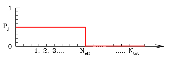
Figure 4.: A schematic representation of $N_{\rm eff}$, defined in our statistical experiment as the maximum number of “switched-on” cells, each containing one star of fixed luminosity $\ell_{\rm eff}$, such as to provide the total observed luminosity of the population, $L_{\rm tot}$, at a given photometric band.

Accordingly, from a statistical point of view, $N_{\rm eff}$ represents therefore the maximum number of bright stars, of constant luminosity $\ell_{\rm eff}$, allowed in a population of $N_{\rm tot}$ members to provide the total luminosity $L_{\rm tot}$ (see Fig. 4). Ideally, this statistical definition assumes a “two-state” condition for sample stars, with $N_{\rm eff}$ “switched-on” objects of $\ell_{\rm eff}$ individual luminosity and the remaining $(N_{\rm tot}-N_{\rm eff})$ “switched-off” stars with $\ell=0$. Alternatively, $N_{\rm eff}$ can also be regarded as the maximum number of states (i.e. “switched-on” cells in our previous example) available to the system, and this straightforwardly leads to a more general extension of the “entropy” ($S$) concept, that in our framework can now be defined as

$$S=\log(N_{\rm eff}/N_{\rm tot}).$$ (11)

or, in its usual thermodynamical notation,

$$\Delta S=\Delta\log N_{\rm eff}$$ (12)

as we would better like to single out its variation within a stellar population rather than its absolute value.

According to our normalization, as $0<N_{\rm eff}(\lambda)/N_{\rm tot}\leq 1$, $S$ is always a negative quantity, depending on wavelength and tipping at zero, in case of a “maximum-entropy” stellar system, where all stars contribute with the same luminosity at a given photometric band.

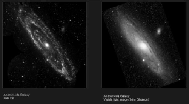
Figure 5.: The centermost $3\hbox{${}^{\circ}$}\times 3\hbox{${}^{\circ}$}$ region of the Andromeda galaxy (M 31), as imaged by the ultraviolet space telescope GALEX (Thilker et al. 2005) between 1500 and 3000 Å (left panel), and seen at optical wavelength (right panel). The image is courtesy of the GALEX scientific team, and made available at the Project Web site http://www.galex.caltech.edu/. It is evident the increased “transparency” of the galaxy at ultraviolet wavelength, as a consequence of a drastically lower number of effective stellar contributors. See text for a discussion.

4. Crowding effects and apparent opacity of stellar systems

As shown in Fig. 3, one striking feature of the $N_{\rm eff}$ function (and its derived entropy quantity) is its wide change with wavelength. In particular, one sees that for a 15 Gyr simple stellar population (SSP) model, from Buzzoni (1993), the entropy peaks around blue/visual wavebands ($UBV$), while the number of effective contributors dramatically drops by nearly five orders of magnitude when moving to short wavelength, below 3000 Å. A similar (although much milder) trend is also evident at infrared wavelength, where $N_{\rm eff}$ smoothly decreases by about one dex, compared to the optical range.

Scaled to a typical $10^{11}$ L_⊙ galaxy, this means that, by looking at mid- ultraviolet wavelength, we have to expect a thin plot of some $10^{4}$ UV-bright stars tracing the galaxy body, compared to a quite smooth surface brightness distribution at visual wavelength, provided by about $10^{10}$ effective stellar contributors. The Andromeda galaxy, as imaged in the visible light and by the ultraviolet space telescope GALEX (Thilker et al. 2005), is a good example in this sense (see Fig. 5).

The exact trend of $N_{\rm eff}$ (and $S$) vs. wavelength is a natural output of theoretical codes for population synthesis, and it can easily be computed for a wide range of the distinctive evolutionary parameters for a stellar population. Detailed values for SSP grids of models can be found in Buzzoni (1993, and Web updates at http://www.bo.astro.it/ eps/home.html) and Cerviño et al. (2002).

The knowledge of the entropy level is of special importance in order to quantitatively assess the expected crowding conditions or rather the apparent “optical depth”, when observing a distant stellar system at different photometric bands. The latter will depend in fact on the effective number of stellar contributors convolved with the instrumental kernel (telescope diffraction pattern plus seeing PSF) that degrades our resolution leading to a smooth nearly “solid” surface brightness profile.

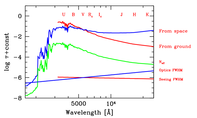
Figure 6.: The apparent system opacity ($\tau$) in case of a SSP as in Fig. 3, assuming to observe the stellar sample from ground and from space (upper curves). Crowding conditions are mainly modulated by seeing, in case of ground-based observations with conventional telescopes, and by the telescope diffraction limit in case of space imaging. Note that calculations for ground-based observations have been stopped shortward of 3000 Å given the atmosphere opacity. In addition, the two curves have been offset by an arbitrary quantity in the logarithm domain to match at the $V$ band. Due to an opposite trend of seeing and optics FWHM (see the two curves at the bottom, as labeled), the convolution with the apparent surface density of stars ($N_{\rm eff}$ curve) leads to different performance outputs. In particular, ground-based observations sensibly improve when moving at longer wavelength, thanks to a more favorable seeing condition, while crowding conditions are expected to maintain roughly constant at the different photometric bands in case of space observations. The Johnson/Cousins photometric band system is reported at the top of the figure, as a reference.

In case of ground-based (i.e. seeing limited) imaging of a star cluster, for instance, the apparent optical depth ($\tau$) is expected to scale as

$$\log\tau_{\rm ground}=S+\log{{\pi\,{\rm FWHM}_{\rm seeing}^{2}}\over{{\rm Cluster~{}apparent~{}area}}}+{\rm const}.$$ (13)

If, on the contrary, we are observing from space (that is fully exploting the telescope diffraction limit), then target opacity will scale as

$$\log\tau_{\rm space}=S+\log{{\pi\,{\rm FWHM}_{\rm Airy}^{2}}\over{{\rm Cluster~{}apparent~{}area}}}+{\rm const}.$$ (14)

In this framework, the difference between a “crowded field” and a “surface brightness fluctuation” is just a matter of apparent “opacity” of the stellar system, eventually depending whether $\tau$ is respectively $\ll 1$ or $\gg 1$.

According to the trend envisaged in Fig. 1, the expected performance of our observations will therefore change with $\lambda$ as in Fig. 6. In general, we see that ground-based observations are more sensitive to the observing photometric band as stars will more easily be picked up at longer wavelength, taking advantage of seeing improvement; on the contrary, our output will not be so critically constrained when observing from space, as the lower value of $N_{\rm eff}$ at infrared wavelength barely compensates the poorer telescope resolving power (compared to the visible wavelength range), thus maintaining the crowding conditions roughly unchanged along the different photometric bands.

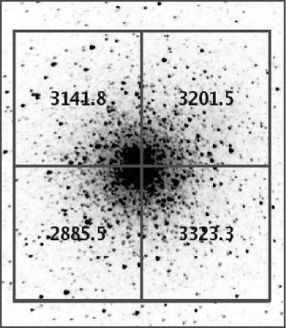
Figure 7.: An illustrative example of surface brightness fluctuations in the globular clsuter M 53 (alias NGC 5024). The $R_{c}$-band frame has been taken at the 2.12m telescope of Cananea (Mexico) with a FOSC camera. Field is roughly $6.5\hbox{${}^{\prime}$}\times 6.5\hbox{${}^{\prime}$}$ sampled with a $1\hbox{${}^{\prime\prime}$}$ pixel size of on the sky. For our experiment, the cluster has been divided in four quadrants reporting the sky-subtracted integrated CCD counts for each partition, as labeled on the plot. See text for discussion.

5. Surface brightness fluctuations

The previous arguments in our discussion make easier now a different statistical approach to the problem of surface brightness fluctuations in stellar systems. In particular, relying on our definition of “fair statistical realization” of a stellar sample (see Sec. 3), one could take advantage of cluster and galaxy symmetry for a different and more general statement of the Tonry & Schneider (1988) method.

For example, in case of a globular cluster, like the $R_{c}$-band CCD picture of M 53 shown in Fig. 7, one could assume that any quadrant of the system (by centering on the photometric barycenter of the cluster) collects a “statistically fair sample” of the whole cluster population, in force of the claimed central symmetry of the system. So, while, in average, each quadrant will display a mean luminosity $L^{\prime}=L_{\rm tot}/4$, a scatter has to be expected for this quantity, according to l.h. side of eq. (7), simply measured as the variance of the four count determinations. In the specific case of Fig. 7 we have

$$\left\{\begin{array}[]{ll}L^{\prime}=3138\quad{\rm counts}\\ \sigma^{2}(L^{\prime})=184^{2}\quad{\rm counts}.\end{array}\right.$$ (15)

The apparent ($R_{c}$-band) effective magnitude ($m_{\rm eff}$) of the M 53 stellar population becomes therefore

$$m_{\rm eff}=-2.5\,\log{\ell_{\rm eff}\over{4\,\pi\,d^{2}}}=-2.5\,\log\left({\sigma^{2}(L^{\prime})\over L^{\prime}}\,{1\over{4\,L^{\prime}}}\right)+M_{R}(\rm M\,53),$$ (16)

being $L_{\rm tot}=4\,L^{\prime}$ the apparent luminosity of the cluster (i.e. across the four quadrants, in CCD counts), to be calibrated in magnitude scale through the known apparent $R_{c}$-band magnitude of M 53 [$M_{R}(\rm M\,53)=7.11$, from Harris (1996), dereddened assuming a color excess $E(B-V)=0.02$ and $A(R_{c})=2.6E(B-V)$ from Moro & Munari (2000)]. Replacing the relevant quantities, for our cluster we have $m_{\rm eff}=14.78$ mag.

For the M 53 stellar population, the Buzzoni (1989, 1993) SSP models predict and absolute ($R_{c}$-band) effective magnitude $M_{\rm eff}=-1.58$ mag, assuming an age of $\sim 15$ Gyr for the cluster, a metallicity [Fe/H] $=-1.88\pm 0.2$ dex (Santos & Piatti 2004) and a blue horizontal branch (HB) morphology. This eventually leads to an estimated distance modulus for M 53 of

$$m_{\rm eff}-M_{\rm eff}=14.78+1.58=+16.36~{}{\rm mag}$$ (17)

in quite good agreement with the standard value of $(m-M)=16.25$ mag from the Harris (1996) globular cluster catalog; this implies a $\sim 5$% relative uncertainty in the derived distance of the cluster with our method.

5.1. Color fluctuations and stellar sampling

Previous application of cluster “fair sampling” basically relies on the claimed symmetry of the system. In this regard, our adopted 4-quadrant partition is fully arbitrary, as any other geometrical combination, like slices of fixed angular aperture, or other fixed-size apertures symmetrically located around the center could work equally well in our method.

As an interesting variant on this line, that may more suitably apply to fully unresolved galaxies, one could also consider to trace the luminosity variance along a given isophote of the surface brightness profile. This could easily be done, for instance, in case of ellipticals or face-on spirals.

One important consequence of the finite luminosity sampled per pixel resolution element, along a given galaxy isophote, is that some intrinsic variance of the apparent color has to be expected, as a consequence of a different photometric entropy with varying the observing band. The amplitude of this color scatter depends on the amount of bolometric $L_{\odot}$ sampled per pixel and the relative variation of $N_{\rm eff}$ at the different photometric bands.

An example is done in Fig. 8, where we computed the statistical variation of the integrated B-V color versus sampled luminosity. The B-V variance (in magnitude scale) derives from

$$\sigma^{2}(B-V)=\sigma^{2}(B)+\sigma^{2}(V)-2\rho\,\sigma(B,V)$$ (18)

where $\sigma^{2}(B)=1/N_{\rm eff}^{B}$, $\sigma^{2}(V)=1/N_{\rm eff}^{V}$, and the covariance term $-2\rho\,\sigma(B,V)$ ranges between zero (if the $B$ and $V$ luminosity contributors can be assumed to be totally independent, that is for a correlation coefficient $\rho=0$ in eq. 18), and $-2\sigma(B)\sigma(V)$ if we assume a perfect positive correlation between the two photometric bands (i.e. assuming $\rho=1$). As shown in Fig. 8, the full variation range for the statistical fluctuation of the integrated color can eventually be written as

$$\mid\sigma(B)-\sigma(V)\mid\,\leq\sigma(B-V)\leq\sqrt{\sigma^{2}(B)+\sigma^{2}(V)}$$ (19)

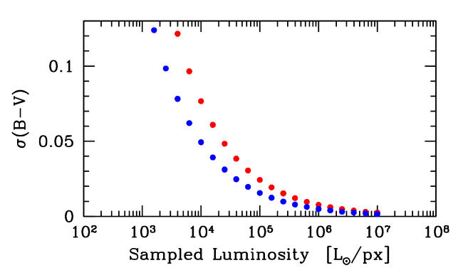
Figure 8.: The expected statistical scatter in the galaxy B-V color versus pixel luminosity sampling. The scatter amount ranges according to eq. (19). High-$S/N$ (i.e. $S/N\gg 100$) high-resolution galaxy imagery could in principle detect the effect.

Quite interestingly, one sees from the figure that a detectable color scatter could be measured along a galaxy surface isophote providing to collect high-($S/N$) (i.e. $S/N\gg 100$) high-resolution imagery. For example, in case of a typical $10^{11}$ L_⊙ elliptical galaxy at the Virgo distance ($d\simeq 15$ Mpc), one expects to sample roughly $10^{5}$ L_⊙/px with a CCD of $\sim 0.2\hbox{${}^{\prime\prime}$}$ pixel size. This leads to a fully measurable $\sigma(B-V)$ scatter of some 0.01 mag (see Fig. 8). The possible cosmological relevance of this test is obvious, as from a measure of a color scatter in a distant galaxy we can derive an absolute estimate of the sampled luminosity, to be compared with the observed surface brightness and derive therefrom the luminosity distance.

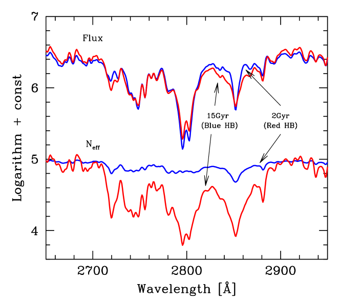
Figure 9.: Theoretical spectral energy distribution (upper plots) and effective stellar contributors ($N_{\rm eff}$) (lower plots) for two SSPs of solar metallicity and Salpeter IMF according to Buzzoni (1989, 1993) population synthesis models. The models refer to a 2 Gyr SSP with red HB morphology, and a 15 Gyr population with blue HB, as labeled. The new Uvblue theoretical library of spectra (Rodriguez-Merino et al. 2005) has been used to reproduce the spectral region around the striking Mgii and Mgi features, about 2800 Å. In spite of a substantially indistiguishable difference between the spectra, the two SSPs display a large difference in terms of effective contributors and photometric entropy, with a much higher statistical scatter in the spectral features expected for the older SSP.

6. Diagnostic tools for high-resolution spectroscopy

Following a substantially similar argument as for the color statistical scatter of previous section, one could also further expand the approach including spectroscopy. Again, the change of $S$ and $N_{\rm eff}$ along wavelength is the key issue that leads us to expect some variance among the spectral features, even at close wavelength difference.

A confident assessment of this effect could be extremely useful as an additional interpretative tool to disentagle the well recognized degeneracy among the evolutionary parameters of stellar populations (see, e.g. the long-lasting question of the “age-metallicity” dilemma as discussed, for instance, by Renzini & Buzzoni 1986 and Buzzoni 1995).

Figure 9 is an illuminating example of this kind of problem. The two plots in the figure display the ultraviolet spectral energy distribution and effective number of stellar contributors for two SSPs of different age and HB morphology. The models have been obtained by matching the Buzzoni (1989) synthesis code with the new Uvblue theoretical spectral library of Rodriguez-Merino et al. (2005).

In particular, a young (2 Gyr) population with red HB morphology is compared with an old (15 gyr) one, with a blue HB. One sees that, in spite of the striking age difference, the two spectra are nearly identical as, in both cases, we have a dominating component of warm stars ($T_{\rm eff}\sim 10\,000$ K) that emit in the ultraviolet range. However, while in the 2 Gyr SSP the UV-luminosity is provided by a large number of main sequence turn-off stars, in the 15 Gyr case we have a prevailing contribution from a few bright stars in the blue tail of the HB.

This has a direct impact on the value of $N_{\rm eff}$, with a much larger scatter along wavelength for the oldest SSP. As a consequence, in the latter case we should likely expect a larger variance (about a factor of two) in the measure of any narrow-band spectrophotometric index along the galaxy isophotes [including both the popular Lick indices of Worthey et al. (1994), in the optical range or the Fanelli et al. (1990) ultraviolet indices], in a way very similar to what we have shown for the B-V color.

Acknowledgments.

It is a pleasure to thank the organizers, David Valls-Gabaud and Miguel Chavez, for their kind invitation to attend this exciting workshop.

References

- Buzzoni (1989) Buzzoni, A. 1989, ApJS, 71, 817
- Buzzoni (1993) Buzzoni, A. 1993, A&A, 275, 433
- Buzzoni (1995) Buzzoni, A. 1995, ApJS, 98, 69
- Cerviño & Luridiana (2004) Cerviño, M. & Luridiana, V. 2004, 413, 145
- Cerviño, Luridiana & Castander (2000) Cerviño, M., Luridiana, V. & Castander, F. J. 2000, A&A, 360, 5
- Cerviño et al. (2001) Cerviño, M., Gómez-Flechoso, M. A., Castander, F. J., Schaerer, D., Mollá, M., Knödlseder, J. & Luridiana, V. 2001, A&A, 376, 422
- Cerviño et al. (2002) Cerviño, M., Valls-Gabaud, D., Luridiana, V. & Mas-Hesse, J. M. 2002, A&A, 381, 51
- Fanelli et al. (1990) Fanelli, M.N., O’Connell, R.W., Burstein, D. & Wu, C.C. 1990, 364, 272
- Harris (1996) Harris, W.E. 1996, AJ, 112, 1487
- Moro & Munari (2000) Moro, D. & Munari, U. 2000, A&AS, 147, 361
- Renzini & Buzzoni (1986) Renzini, A. & Buzzoni, A. 1986 in Spectral evolution of galaxies, eds. C. Chiosi & A. Renzini (Dordrecht: Reidel) p. 195
- Rodriguez-Merino et al. (2005) Rodriguez-Merino, L.H., Chavez, M., Bertone, E. & Buzzoni, A. 2005, ApJ, 626, 411
- Santos & Piatti (2004) Santos, J.F.C. Jr. & Piatti, A.E. 2004, A&A, 428, 79
- Thilker et al. (2005) Thilker, D.A., Hoopes, C.G., Bianchi, L., et al. 2005, ApJ, 619, L67
- Tonry (1991) Tonry, J.L. 1991, ApJ, 373, L1
- Tonry & Schneider (1988) Tonry, J.L., & Schneider, D.P. 1988, AJ, 96, 807
- Worthey et al. (1994) Worthey, G., Faber, S. M., Gonzalez, J.J. & Burstein, D. 1994, ApJS, 94, 687
- Wynne (1999) Wynne, C.G. 1999, MNRAS, 302, 830