Estimated IR and phosphorescence emission fluxes for specific Polycyclic Aromatic Hydrocarbons in the Red Rectangle

Following the tentative identification of the blue luminescence in the Red Rectangle by Vijh et al. (2005), we compute absolute fluxes for the vibrational IR emission and phosphorescence bands of three small polycyclic aromatic hydrocarbons. The calculated IR spectra are compared with available ISO observations. A subset of the emission bands are predicted to be observable using presently available facilities, and can be used for an immediate, independent, discriminating test on their alleged presence in this well–known astronomical object.

1 Introduction

Recently, Vijh et al. (2004) detected a blue luminescence (BL) in the well–known bipolar protoplanetary Red Rectangle (RR) nebula (Cohen 1975; Cohen et al. 2004). Shortly thereafter, Vijh et al. (2005), after a thorough analysis of the extinction properties and of the correlation of the BL with the observed near–IR emission at 3.3 $\mu$m, concluded that they are both most likely due to small, neutral polycyclic aromatic hydrocarbons (PAHs), composed of three to four aromatic units. Another possible explanation of the BL tentatively identifies it as fluorescence by ultrasmall silicon nanoparticles (Nayfeh et al. 2005).

The hypothesis of the ubiquitous presence of free gas–phase PAHs in the interstellar medium (ISM) originated about 20 years ago (Léger & Puget 1984; Allamandola et al. 1985). Due to their spectral properties and their high photostability, these molecules were suggested as the most natural interpretation for the so–called “Aromatic Infrared Bands” (AIBs), a set of emission bands observed near 3.3, 6.2, 7.7, 8.6, 11.3 and 12.7 $\mu$m, in many dusty environments excited by UV photons (Léger et al. 1989; Allamandola et al. 1989). The AIBs are the spectral fingerprint of the excitation of vibrations in aromatic C–C and C–H bonds (Duley & Williams 1981). Furthermore, PAHs and their cations were also supposed to account for a subset of the “Diffuse Interstellar Bands” (DIBs) (Léger & d’Hendecourt 1985; van der Zwet & Allamandola 1985; Crawford et al. 1985), more than $\sim 300$ absorption features ubiquitously observed in the near-UV, visible and near-IR in the spectra of reddened stars (see e. g. Ehrenfreund & Charnley 2000, and references therein).

The RR nebula, besides being one of the brightest sources of AIBs in the sky, also has the almost unique property of displaying a subset of emission bands in the visible (Schmidt et al. 1980; Van Winckel et al. 2002) which appear to be associated with a subset of DIBs (Scarrott et al. 1992). The RR and the R CrB star V854 Cen (Kameswara-Rao & Lambert 1993) are the only known cases in which DIBs have ever been possibly observed in emission. This makes the tentative identification of small neutral PAHs in this same nebula a potentially very exciting discovery, with far–reaching consequences also on the long–standing mystery of the identification of DIBs.

However, while the analysis in Vijh et al. (2005) narrows the range of potential carriers of the observed BL to a small number of molecules, it cannot provide a definitive identification, which requires an independent test. Such a test can be obtained from the IR and phosphorescence emission spectrum of the same molecules. The low–frequency vibrational modes (Langhoff 1996; Zhang et al. 1996) and phosphorescence bands (Salinas Castillo et al. 2004) provide an unique signature and ought to be produced together with electronic fluorescence bands (Bréchignac 2005).

We carried out simulations of the photophysics of the candidate molecules using a Monte–Carlo code (Mulas 1998; Joblin et al. 2002; Malloci et al. 2003; Mulas et al. 2003), together with quantum–chemical calculations for the relevant molecular parameters (Langhoff 1996; Martin et al. 1996; Malloci et al. 2004) and available laboratory measurements for the photoabsorption spectra (Joblin et al. 1992; Joblin 1992) and for visible and IR fluorescence quantum yields (Bréchignac 2005). This produces a quantitative prediction of the IR and phosphorescence emission spectra for each given molecule, which must be related to the integrated BL attributed to this same molecule.

2 Modelling procedure

In previous papers (Joblin et al. 2002; Malloci et al. 2003; Mulas et al. 2003) we demonstrated the use of Monte–Carlo models to simulate the detailed photophysics of a specific PAH embedded in a given radiation field (RF). We here apply the same procedure to the specific case of the three small, neutral PAHs which were tentatively identified in the Red Rectangle nebula by Vijh et al. (2005), namely anthracene (C₁₄H₁₀), phenanthrene (C₁₄H₁₀) and pyrene (C₁₆H₁₀) to derive their expected complete IR emission spectra.

For the modelling procedure we used quantum–chemical results for structural parameters and vibrational analysis, both from the literature (Langhoff 1996; Martin et al. 1996) and obtained by ourselves. For anthracene and pyrene we used the experimental photo–absorption cross–sections from Joblin et al. (1992); Joblin (1992), while for phenanthrene we used the theoretical spectrum from Malloci et al. (2004). We performed all of the quantum–chemical calculations in the framework of the Density Functional Theory (DFT), using the Octopus and NWChem computational codes. Details on them can be found elsewhere (Malloci et al. 2004, 2005).

A crucial modelling parameter is the assumed knowledge of the relaxation paths of the modelled molecules upon electronic excitation following a photon absorption. Almost all neutral PAHs, including in particular anthracene, phenanthrene and pyrene, upon excitation $\mathrm{S}_{n}\leftarrow\mathrm{S}_{0}$, are well–known to undergo very fast internal conversion (IC) to the $\mathrm{S}_{1}$ electronic level (see e. g. Leach 1995, and references therein). From there, three relaxation paths are available, their relative weights dependent on the vibrational energy available:

1. fluorescence $\mathrm{S}_{1}\to\mathrm{S}_{0}$ with a permitted electronic transition, the remaining energy being subsequently radiated by vibrational transitions in $\mathrm{S}_{0}$; relaxation of small PAHs via this path is the proposed origin of BL in the RR (Vijh et al. 2004, 2005);

2. direct $\mathrm{S}_{1}\leadsto\mathrm{T}_{1}$ or indirect $\mathrm{S}_{1}\leadsto\mathrm{T}_{n}\leadsto\mathrm{T}_{1}$ intersystem crossing (ISC), a radiationless transition followed by the emission of a phosphorescence photon in a $\mathrm{T}_{1}\to\mathrm{S}_{0}$ spin–forbidden, electronic–permitted transition; the remaining energy is radiated in vibrational transitions either (almost always) from $\mathrm{S}_{0}$ after the phosphorescence transition or (very seldom) from $\mathrm{T}_{1}$ before it;

3. internal conversion $\mathrm{S}_{1}\leadsto\mathrm{S}_{0}$, a radiationless transition, after which essentially all excitation energy is radiated by vibrational transitions.

According to experimental results (Bréchignac 2005), the rate of fluorescence transitions (1) is essentially independent of the excitation energy. The rate of ISC radiationless transitions (2) increases slightly with excitation energy for the three molecules considered. The relaxation path (3) by IC to the ground state is open only when some excess vibrational energy in $\mathrm{S}_{1}$ is available, such threshold depending on the specific molecule and varying from $\sim 2\,\,10^{3}$ cm^-1 for anthracene to $\sim 4\,\,10^{4}$ cm^-1 for pyrene. Above this threshold the rate of IC to $\mathrm{S}_{0}$ (3) exponentially increases, becoming by and large the dominant relaxation path. The energy–dependent quantum yields for these three relaxation paths were measured in gas–phase experiments by Bréchignac (2005) for all the three molecules under study here.

All of the three relaxation paths described above contribute to IR emission from the ground $\mathrm{S}_{0}$ electronic state and are therefore considered in our model. Even the slowest electronic transition, i. e. the $\mathrm{T}_{1}\to\mathrm{S}_{0}$ involved in phosphorescence, occurs with decay constants of the order of, at most, $\tau_{\mathrm{ph}}\sim 1.5\,\,10^{-3}$ s (Salinas Castillo et al. 2004), while the time constant involved in the fastest vibrational transitions is always $\tau_{\mathrm{IR}}\gtrsim 5\,\,10^{-2}$ s. This ensures that vibrational relaxation almost always occurs after any electronic transition in the relaxation path, i. e. from $\mathrm{S}_{0}$. Along any of the three relaxation paths described above, the only process which can to some extent compete with the IR emission is the absorption of another UV–visible photon before the end of the vibrational cascade. When this happens, the residual excitation energy is added to that of the newly absorbed photon, making available higher–energy vibrational modes. Emission in the weakest IR bands, mostly towards the low–energy end, essentially happens only when the stronger ones, mostly towards the high–energy end, are energetically unaccessible; if vibrational cascades are interrupted before their end, weak bands are consequently suppressed, in favour of the stronger ones, which are emitted much more quickly when the molecule excitation energy is high enough.

We considered the modelled molecules in two different regions of the nebula and, therefore, our simulations correspond to two different exciting RFs. The first one is a Kurucz spectrum with effective temperature T = 8250 K, surface gravity $\log g=1.5$ and total luminosity of 6050 L_⊙ (Vijh et al. 2005), summed with a blackbody at T = 60000 K to represent the He white dwarf companion with a total luminosity of 100 L_⊙ (Men’shchikov et al. 2002), both truncated at the Lyman limit and diluted according to the geometry of the source (Men’shchikov et al. 2002) at given angular distances along the polar axes of the nebula. Extinction along the polar axes of the nebula is low and particularly gray (Men’shchikov et al. 2002; Vijh et al. 2005) and we neglect it altogether. We will therefore assume the spectrum of the estimated RF to be constant along the bipolar lobes, and just scale with a wavelength–independent factor with distance, in the wavelength range which pumps the BL.

The second RF we considered is the “attenuated” one, as shown in Vijh et al. (2005), corresponding to what is seen by a molecule in the halo of the RR nebula, out of the bipolar cones and out of the dense, optically thick torus–like dust shell surrounding the central binary star. This RF is essentially due to heavily obscured light leaking through the torus and to light initially directed along the bipolar lobes and subsequently scattered into the halo. Since the halo itself is optically very thin (Men’shchikov et al. 2002; Vijh et al. 2005), we again assume the spectrum of this RF to be constant and just scale with a wavelength–independent factor with distance, over the energy range which pumps the BL.

Both RFs are limited on the high–energy side by the Lyman limit at 13.6 eV, since higher energy photons are completely absorbed in a small H_II region close to the central evolved star (Men’shchikov et al. 2002). Photons of energies lower than the absorption edge of the first permitted electronic transition, which for small, neutral PAHs is always higher than $\sim$2 eV, are irrelevant for our purposes. The branching ratios for the three main relaxation channels following UV/visible photon absorption by anthracene, phenanthrene and pyrene in the two RFs considered are listed in Table 1. For the sake of completeness, we also included the ionisation yields, estimated according to the formula given by Le Page et al. (2001), using the ionisation potentials 7.439 eV for anthracene, 7.891 eV for phenanthrene and 7.426 eV for pyrene taken from the online NIST chemistry WebBook (Lias 2005).

Table 1: Computed branching ratios for the three main relaxation channels following UV/visible photon absorption by anthracene, phenanthrene and pyrene in the RF of the lobes and halo of the RR nebula (see text for details).

	Relaxation branching ratios
	fluorescence	I. S. C.	I. C.	ionisation
	$(\mathrm{S}_{1}\to\mathrm{S}_{0})$	$(\mathrm{S}_{1}\leadsto\mathrm{T}_{1})$	$(\mathrm{S}_{1}\leadsto\mathrm{S}_{0})$
Anthracene (C14H10)
lobes	0.157	$\ll 10^{-3}$	0.827	0.016
halo	0.203	$\ll 10^{-3}$	0.796	0.001
Phenanthrene (C14H10)
lobes	0.031	0.372	0.587	0.010
halo	0.042	0.562	0.396	$3\,\,10^{-5}$
Pyrene (C16H10)
lobes	0.060	0.284	0.642	0.014
halo	0.094	0.408	0.497	0.001

Under these conditions, the number $\displaystyle\frac{dR_{\mathrm{bl}}(\nu^{\prime})}{d\nu^{\prime}}$ of BL photons radiated per unit time by a given molecule in the frequency interval between $\nu^{\prime}$ and $\nu^{\prime}+d\nu^{\prime}$ will be proportional to the respective fluorescence quantum yield $\displaystyle\frac{dQ_{\mathrm{fl}}(\nu,\nu^{\prime})}{d\nu^{\prime}}$, multiplied by the rate of absorption of exciting photons, in turn given by the product of the flux of exciting photons $F_{\mathrm{exc}}(\nu)$ times the absorption cross–section $\sigma(\nu)$ of the molecule, i. e.

$$\frac{dR_{\mathrm{bl}}(\nu^{\prime})}{d\nu^{\prime}} = \int d\nu F_{\mathrm{exc}}(\nu)\sigma(\nu)\frac{dQ_{\mathrm{fl}}(\nu,\nu^{\prime})}{d\nu^{\prime}}$$

$$= \overline{F}_{\mathrm{exc}}\int d\nu\Phi_{\mathrm{exc}}(\nu)\sigma(\nu)\frac{dQ_{\mathrm{fl}}(\nu,\nu^{\prime})}{d\nu^{\prime}}$$

$$= \overline{F}_{\mathrm{exc}}\frac{d\overline{\sigma}_{\mathrm{fl}}(\nu^{\prime})}{d\nu^{\prime}},$$

where we defined

$$\overline{F}_{\mathrm{exc}}=\int d\nu F_{\mathrm{exc}}(\nu),\qquad\Phi_{\mathrm{exc}}(\nu)=\frac{F_{\mathrm{exc}}(\nu)}{\overline{F}_{\mathrm{exc}}}$$

$$\mathrm{and}\quad\frac{d\overline{\sigma}_{\mathrm{fl}}(\nu^{\prime})}{d\nu^{\prime}}=\int d\nu\Phi_{\mathrm{exc}}(\nu)\sigma(\nu)\frac{dQ_{\mathrm{fl}}(\nu,\nu^{\prime})}{d\nu^{\prime}}.$$

With the assumptions we made for the RFs, $\overline{F}_{\mathrm{exc}}$ will vary with the position in the nebula, while $\Phi_{\mathrm{exc}}(\nu)$, which contains the frequency dependence of $F_{\mathrm{exc}}(\nu)$, will only vary between the biconic lobes and the halo but will be position–independent within each of them. Since $\displaystyle\frac{dQ_{\mathrm{fl}}(\nu,\nu^{\prime})}{d\nu^{\prime}}$ is independent of the photon absorption rate, $\displaystyle\frac{d\overline{\sigma}_{\mathrm{fl}}(\nu^{\prime})}{d\nu^{\prime}}$ does not depend on the position along the line of sight.

Completely analogous equations can be written for the IR emission and phosphorescence, i. e.

$$\frac{dR_{\mathrm{IR}}(\nu^{\prime})}{d\nu^{\prime}} = \overline{F}_{\mathrm{exc}}\int d\nu\Phi_{\mathrm{exc}}(\nu)\sigma(\nu)\frac{dQ_{\mathrm{IR}}(\nu,\nu^{\prime})}{d\nu^{\prime}}$$

$$= \overline{F}_{\mathrm{exc}}\frac{d\overline{\sigma}_{\mathrm{IR}}(\nu^{\prime})}{d\nu^{\prime}}$$

$$\mathrm{with}\quad\frac{d\overline{\sigma}_{\mathrm{IR}}(\nu^{\prime})}{d\nu^{\prime}}=\int d\nu\Phi_{\mathrm{exc}}(\nu)\sigma(\nu)\frac{dQ_{\mathrm{IR}}(\nu,\nu^{\prime})}{d\nu^{\prime}}$$

and

$$\frac{{dR}_{\mathrm{{ph}}}{(\nu^{\prime})}}{{d\nu^{\prime}}} {=} {\overline{F}}_{\mathrm{{exc}}}{\int d\nu\Phi}_{\mathrm{{exc}}}{(\nu)\sigma(\nu)}\frac{{dQ}_{\mathrm{{ph}}}{(\nu,\nu^{\prime})}}{{d\nu^{\prime}}}$$

$${=} {\overline{F}}_{\mathrm{{exc}}}\frac{{d\overline{\sigma}}_{\mathrm{{ph}}}{(\nu^{\prime})}}{{d\nu^{\prime}}}$$

$$\mathrm{{with}}\quad\frac{{d\overline{\sigma}}_{\mathrm{{ph}}}{(\nu^{\prime})}}{{d\nu^{\prime}}}{=\int d\nu\Phi}_{\mathrm{{exc}}}{(\nu)\sigma(\nu)}\frac{{dQ}_{\mathrm{{ph}}}{(\nu,\nu^{\prime})}}{{d\nu^{\prime}}}.$$

As explained above, $\displaystyle\frac{dQ_{\mathrm{IR}}(\nu,\nu^{\prime})}{d\nu^{\prime}}$ does slightly depend on the photon absorption rate if the average time between photon absorptions is smaller than the average time it takes for an excited molecule to complete its IR emission cascade. This is not the case for $\displaystyle\frac{dQ_{\mathrm{ph}}(\nu,\nu^{\prime})}{d\nu^{\prime}}$, since phosphorescence, although slower than fluorescence, still occurs on a much shorter timescale than the average interval between two photon absorptions in all cases considered here. The detailed three–dimensional distribution of the molecules supposedly emitting the BL along a given line of sight is unknown: the emitting molecules might equally well be concentrated close to the source, where their photon absorption rate would be higher, or in a large volume extending relatively far out, with correspondingly lower photon absorption rates. We therefore considered a range of distances to the central source, and hence of photon absorption rates, evaluating the corresponding variation of $\displaystyle\frac{dQ_{\mathrm{IR}}(\nu,\nu^{\prime})}{d\nu^{\prime}}$ and of the calculated IR emission spectra.

Under optically thin conditions the observed fluorescence photon flux per unit solid angle on the sky along a given direction is given by:

$$\frac{dF_{\mathrm{bl}}(\nu^{\prime})}{d\Omega} = \frac{1}{4\pi}\int drn(r)\frac{dR_{\mathrm{bl}}(r,\nu^{\prime})}{d\nu^{\prime}}$$

$$= \frac{1}{4\pi}\frac{d\overline{\sigma}_{\mathrm{fl}}(\nu^{\prime})}{d\nu^{\prime}}\int drn(r)\overline{F}_{\mathrm{exc}}(r)$$

$$= \frac{1}{4\pi}\frac{d\overline{\sigma}_{\mathrm{fl}}(\nu^{\prime})}{d\nu^{\prime}}\Upsilon,$$

with the definition

$$\Upsilon=\int drn(r)\overline{F}_{\mathrm{exc}}(r).$$ (5)

Equation (2) assumes $\displaystyle\frac{d\overline{\sigma}_{\mathrm{fl}}(\nu^{\prime})}{d\nu^{\prime}}$ to be constant along the line of sight, which is appropriate for a line of sight traversing only the halo of the RR. For a line of sight going through both the halo and one of the biconical lobes, the integral over the line of sight can be split in a part in the lobe and a part in the halo, in each of which $\displaystyle\frac{d\overline{\sigma}_{\mathrm{fl}}(\nu^{\prime})}{d\nu^{\prime}}$ is constant. Equation (2) can be thus generalised to

$$\frac{dF_{\mathrm{bl}}(\nu^{\prime})}{d\Omega}=\frac{1}{4\pi}\left(\frac{d\overline{\sigma}_{\mathrm{fl}}^{\mathrm{lobe}}(\nu^{\prime})}{d\nu^{\prime}}\Upsilon_{\mathrm{lobe}}+\frac{d\overline{\sigma}_{\mathrm{fl}}^{\mathrm{halo}}(\nu^{\prime})}{d\nu^{\prime}}\Upsilon_{\mathrm{halo}}\right),$$ (6)

where $\Upsilon_{\mathrm{lobe}}$ and $\Upsilon_{\mathrm{halo}}$ are still defined by Eq. (5), the only difference being the domain of integration, which includes respectively only the part of the line of sight in the lobe or only the part in the halo.

Equivalent equations can be written again for both the IR emission and phosphorescence:

$$\frac{dF_{\mathrm{IR}}(\nu^{\prime})}{d\Omega}=\frac{1}{4\pi}\left(\frac{d\overline{\sigma}_{\mathrm{IR}}^{\mathrm{lobe}}(\nu^{\prime})}{d\nu^{\prime}}\Upsilon_{\mathrm{lobe}}+\frac{d\overline{\sigma}_{\mathrm{IR}}^{\mathrm{halo}}(\nu^{\prime})}{d\nu^{\prime}}\Upsilon_{\mathrm{halo}}\right).$$ (7)

$$\frac{{dF}_{\mathrm{{ph}}}{(\nu^{\prime})}}{{d\Omega}}=\frac{{1}}{{4\pi}}{\left(\frac{{d\overline{\sigma}}_{\mathrm{{ph}}}^{\mathrm{{lobe}}}{(\nu^{\prime})}}{{d\nu^{\prime}}}{\Upsilon}_{\mathrm{{lobe}}}+\frac{{d\overline{\sigma}}_{\mathrm{{ph}}}^{\mathrm{{halo}}}{(\nu^{\prime})}}{{d\nu^{\prime}}}{\Upsilon}_{\mathrm{{halo}}}\right)}.$$ (8)

In Eq. (7) above $\displaystyle\frac{d\overline{\sigma}_{\mathrm{IR}}^{\mathrm{lobe}}(\nu^{\prime})}{d\nu^{\prime}}$ and $\displaystyle\frac{d\overline{\sigma}_{\mathrm{IR}}^{\mathrm{halo}}(\nu^{\prime})}{d\nu^{\prime}}$ are supposed to be effective values, averaged along the line of sight.

The quantities $\displaystyle\frac{d\overline{\sigma}_{\mathrm{fl}}^{\mathrm{lobe}}(\nu^{\prime})}{d\nu^{\prime}}$ and $\displaystyle\frac{d\overline{\sigma}_{\mathrm{fl}}^{\mathrm{halo}}(\nu^{\prime})}{d\nu^{\prime}}$ can be estimated for anthracene, pyrene and phenanthrene using the assumed spectrum of the exciting radiation fields and the quantum yields measured by Bréchignac (2005). If we consider a line of sight dominated either by the lobes or by the halo, we can use the simpler Eq. (2). Integrating both sides of Eq. (2) over $\nu^{\prime}$ we obtain

$$\int d\nu^{\prime}\frac{dF_{\mathrm{bl}}(\nu^{\prime})}{d\Omega} = \frac{\Upsilon}{4\pi}\int d\nu^{\prime}\frac{d\overline{\sigma}_{\mathrm{fl}}(\nu^{\prime})}{d\nu^{\prime}}$$

$$= \frac{\Upsilon}{4\pi}\int d\nu\Phi_{\mathrm{exc}}(\nu)\sigma(\nu)\int d\nu^{\prime}\frac{dQ_{\mathrm{fl}}(\nu,\nu^{\prime})}{d\nu^{\prime}}$$

$$= \frac{\Upsilon}{4\pi}\int d\nu\Phi_{\mathrm{exc}}(\nu)\sigma(\nu)Q_{\mathrm{fl}}(\nu)$$

$$= \frac{\Upsilon}{4\pi}\overline{\sigma}_{\mathrm{fl}}$$

where the right hand side is the integrated BL photon flux due to a given molecule, observed along a given line of sight and $\displaystyle\overline{\sigma}_{\mathrm{fl}}$ is defined by the equation above.

The BL spectrum in the RR has been reported by Vijh et al. (2004) and Vijh et al. (2005). If a fraction $\eta$ of the total, integrated BL photon flux observed is due to a given molecule, we can solve Eq. (2) with respect to $\displaystyle\frac{\Upsilon}{4\pi}$, to yield

$$\frac{\Upsilon}{4\pi}=\frac{\eta}{\overline{\sigma}_{\mathrm{fl}}}\int d\nu\frac{dF_{\mathrm{bl}}(\nu)}{d\Omega}.$$ (10)

This result can be plugged back in Eqs. (7) and (8), from which we obtain respectively

$$\frac{dF_{\mathrm{IR}}(\nu^{\prime})}{d\Omega}=\frac{d\overline{\sigma}_{\mathrm{IR}}(\nu^{\prime})}{d\nu^{\prime}}\frac{{\eta}}{{\overline{\sigma}}_{\mathrm{{fl}}}}\int d\nu\frac{dF_{\mathrm{{bl}}}{(\nu)}}{d\Omega}$$ (11)

$${\frac{dF_{\mathrm{{ph}}}{(\nu^{\prime})}}{d\Omega}=\frac{d\overline{\sigma}_{\mathrm{{ph}}}{(\nu^{\prime})}}{{d\nu^{\prime}}}\frac{{\eta}}{\overline{\sigma}_{\mathrm{fl}}}\int d\nu\frac{dF_{\mathrm{bl}}(\nu)}{d\Omega}.}$$ (12)

Integrating Eq. (12) and proceeding as in Eq. (2) we obtain:

$${\int d\nu^{\prime}\frac{dF_{\mathrm{ph}}(\nu^{\prime})}{d\Omega}} {=} {\int d\nu^{\prime}\frac{d\overline{\sigma}_{\mathrm{ph}}(\nu^{\prime})}{d\nu^{\prime}}\frac{\eta}{\overline{\sigma}_{\mathrm{fl}}}\int d\nu\frac{dF_{\mathrm{bl}}(\nu)}{d\Omega}}$$

$${=} {\eta\frac{\overline{\sigma}_{\mathrm{ph}}}{\overline{\sigma}_{\mathrm{fl}}}\int d\nu\frac{dF_{\mathrm{bl}}(\nu)}{d\Omega}.}$$

The ratio $\displaystyle\frac{\overline{\sigma}_{\mathrm{ph}}}{\overline{\sigma}_{\mathrm{fl}}}$, for a given molecule in a given RF, is simply the ratio of the branching ratios for phosphorescence and fluorescence, as listed in Table 1. The quantities $\displaystyle\frac{d\overline{\sigma}_{\mathrm{IR}}^{\mathrm{lobe}}(\nu^{\prime})}{d\nu^{\prime}}$ and $\displaystyle\frac{d\overline{\sigma}_{\mathrm{IR}}^{\mathrm{halo}}(\nu^{\prime})}{d\nu^{\prime}}$ are part of the results of our Monte–Carlo model. The integrated BL photon flux along the lines of sight at offsets of 2.5”S 2.6”E and 2.5”S 7.8”E from the central source of the RR nebula were obtained from Vijh et al. (2005) and Vijh et al. (2004), assuming an average energy of the BL photons of $\sim$3.1 eV. They are respectively ${\sim 9.2\,\,10^{9}}$ photons s^-1 cm^-2 sr^-1 at 2.5”S 2.6”E and ${\sim 2.5\,\,10^{9}}$ photons s^-1 cm^-2 sr^-1 at 2.5”S 7.8”E.

The line of sight at the offset 2.5”S 7.8”E is completely in the halo of the RR nebula. Therefore in this case, with the exception of $\eta$, all quantities on the right hand side of Eqs. (11) and (12) are known or can be calculated. We can thus quantitatively estimate the expected IR emission and phosphorescence spectrum of anthracene, phenanthrene and pyrene apart from a scaling factor $\eta$.

The line of sight at the offset 2.5”S 2.6”E traverses both the southern lobe and the halo of the RR nebula. Given the geometry of the source (Men’shchikov et al. 2002), the part in the halo of this latter line of sight is very similar to the line of sight at the offset 2.5”S 7.8”E; we hence assume their contributions to both the BL (${\sim 2.5\,\,10^{9}}$ photons s^-1 cm^-2 sr^-1) and the IR emission to be approximately the same. The remaining BL at 2.5”S 2.6”E ($\sim 6.7\,\,10^{9}$ photons s^-1 cm^-2 sr^-1), after subtracting such estimated contribution from the halo, is due to the portion of the line of sight through the lobe. Therefore for this part we can again use Eq. (11), with the RF in the lobes. The total estimated IR emission spectra at 2.5”S 2.6”E can therefore be obtained from the sum of the estimated spectra from the portions of the line of sight respectively through the lobe and through the halo.

3 Results

3.1 IR emission

Tables 2, 3, 4 and 5 list the most intense mid– and far–IR emission bands expected, along with their calculated fluxes, respectively for anthracene (using two different vibrational analyses), phenanthrene and pyrene, assuming each of them, in turn, to be the sole carrier (i. e. $\eta\simeq 1$) of the observed BL at positions 2.5”S 2.6”E and 2.5”S 7.8”E from the central source. These fluxes can be simply scaled by the appropriate factor if the given molecule is assumed to only contribute a fraction of the luminescence. Since the IR fluxes scaled in this way still do slightly depend on the assumed photon absorption rate (see the discussion in the previous section), we ran independent Monte–Carlo simulations assuming a range of different photon absorption rates. In the halo the photon absorption rates turn out to be always small enough to allow almost all vibrational relaxation cascades to finish. This means that the estimated IR emission from the halo is independent of the three–dimensional distribution of the molecules along the line of sight. The situation is slightly different for the lobes. For the closest position to the central source along the line of sight at 2.5”S 2.6”E we estimated an average time between absorptions $\tau_{\mathrm{abs}}\sim{70}$ s for pyrene and $\tau_{\mathrm{abs}}\sim{60}$ s for the other two molecules. We computed the estimated IR emission fluxes for the portion in the lobe of the line of sight at 2.5”S 2.6”E assuming the above absorption rates and those given by an RF dilution by a factor of $\sim 6$, corresponding to molecules distributed farther away from the nebular axis, near the edges of the lobe. It turns out that only the very weakest IR–active bands of each molecule are significantly affected, being somewhat suppressed (up to a factor $\sim$1.6 in the worst case) when using the higher photon absorption rates. For all the other IR–active bands, the resulting variation in the estimated fluxes is smaller than the uncertainty of the calculated vibrational transition intensities we used. To evaluate the impact of the latter uncertainty, we performed two sets of simulations for anthracene, using the DFT vibrational analyses respectively at the B3LYP/4–31G level of theory (Langhoff 1996) for one and at the B3LYP/cc-pvdz (Martin et al. 1996) for the other. The latter is very nearly the best currently feasible for these molecules, while the former is well known to provide a very good compromise between accuracy and computational efficiency (Langhoff 1996; Bauschlicher & Langhoff 1997). The overall agreement between the two calculations is very good: while the two calculations distribute intensities in a slightly different way among nearby vibrational modes, their total is almost the same (see e. g. the in–plane C–H stretches between 3.25 and 3.29 $\mu$m). The differences on single band intensities and positions are comparable to the relative inaccuracy of each of the two upon comparison with available experimental data (Hudgins & Sandford 1998).

The resulting IR emission fluxes are shown respectively in Tables 2 and 3. Upon comparison, they show the accuracy of the vibrational analyses to dominate the uncertainty in the estimated IR emission fluxes.

Table 2: Absolute integrated IR emission fluxes expected for the most intense IR–active bands of anthracene, calculated using the vibrational analysis performed at the B3LYP/4–31G level of theory. They were estimated for two offsets from the central source, with two different RF dilution factors for the position on the lobe (see text for details).

Band pos. ($\mu$m)	Integrated flux/$\eta$ ($\mathrm{W}\mathrm{sr}^{-1}\mathrm{cm}^{-2}$)
	2.5”S 2.6”E		2.5”S 7.8”E
	73% lobe + 27% halo		halo
	high abs. rate	low abs. rate
3.25	$1.1\,\,10^{-8}$	$1.0\,\,10^{-8}$	$2.0\,\,10^{-9}$
3.26	$6.9\,\,10^{-9}$	$6.7\,\,10^{-9}$	$1.3\,\,10^{-9}$
3.28	$2.4\,\,10^{-11}$	$2.2\,\,10^{-11}$	$4.3\,\,10^{-12}$
3.28	$1.8\,\,10^{-9}$	$1.8\,\,10^{-9}$	$3.5\,\,10^{-10}$
3.29	$1.0\,\,10^{-9}$	$1.0\,\,10^{-9}$	$1.9\,\,10^{-10}$
6.16	$1.5\,\,10^{-9}$	$1.5\,\,10^{-9}$	$3.0\,\,10^{-10}$
6.51	$4.2\,\,10^{-10}$	$4.2\,\,10^{-10}$	$8.9\,\,10^{-11}$
6.86	$8.3\,\,10^{-10}$	$8.5\,\,10^{-10}$	$1.8\,\,10^{-10}$
6.86	$3.9\,\,10^{-10}$	$3.9\,\,10^{-10}$	$8.2\,\,10^{-11}$
7.22	$3.0\,\,10^{-11}$	$2.9\,\,10^{-11}$	$6.0\,\,10^{-12}$
7.43	$5.4\,\,10^{-10}$	$5.3\,\,10^{-10}$	$1.1\,\,10^{-10}$
7.60	$8.7\,\,10^{-10}$	$8.5\,\,10^{-10}$	$1.8\,\,10^{-10}$
7.85	$1.1\,\,10^{-9}$	$1.1\,\,10^{-9}$	$2.4\,\,10^{-10}$
8.55	$1.5\,\,10^{-10}$	$1.6\,\,10^{-10}$	$3.3\,\,10^{-11}$
8.62	$4.0\,\,10^{-10}$	$4.0\,\,10^{-10}$	$8.5\,\,10^{-11}$
8.67	$1.0\,\,10^{-9}$	$1.0\,\,10^{-9}$	$2.1\,\,10^{-10}$
9.95	$4.8\,\,10^{-10}$	$4.8\,\,10^{-10}$	$1.1\,\,10^{-10}$
10.41	$8.6\,\,10^{-10}$	$8.7\,\,10^{-10}$	$1.9\,\,10^{-10}$
11.00	$1.9\,\,10^{-10}$	$1.9\,\,10^{-10}$	$4.0\,\,10^{-11}$
11.32	$6.3\,\,10^{-9}$	$6.3\,\,10^{-9}$	$1.4\,\,10^{-9}$
12.56	$2.9\,\,10^{-12}$	$3.4\,\,10^{-12}$	$2.8\,\,10^{-12}$
13.71	$6.2\,\,10^{-9}$	$6.3\,\,10^{-9}$	$1.4\,\,10^{-9}$
15.33	$1.1\,\,10^{-10}$	$1.1\,\,10^{-10}$	$2.6\,\,10^{-11}$
16.34	$5.0\,\,10^{-10}$	$5.1\,\,10^{-10}$	$1.1\,\,10^{-10}$
21.26	$8.9\,\,10^{-10}$	$9.0\,\,10^{-10}$	$2.0\,\,10^{-10}$
26.35	$2.1\,\,10^{-11}$	$2.9\,\,10^{-11}$	$1.7\,\,10^{-11}$
43.68	$9.1\,\,10^{-11}$	$1.3\,\,10^{-10}$	$3.3\,\,10^{-11}$
110.23	$5.0\,\,10^{-11}$	$7.5\,\,10^{-11}$	$4.0\,\,10^{-11}$

Table 3: Absolute integrated IR emission fluxes expected for the most intense IR–active bands of anthracene, calculated using the vibrational analysis performed at the B3LYP/cc–pvdz level of theory (Martin et al. 1996). They were estimated for two offsets from the central source, with two different RF dilution factors for the position on the lobe (see text for details).

Band pos. ($\mu$m)	Integrated flux/$\eta$ ($\mathrm{W}\mathrm{sr}^{-1}\mathrm{cm}^{-2}$)
	2.5”S 2.6”E		2.5”S 7.8”E
	73% lobe + 27% halo		halo
	high abs. rate	low abs. rate
3.26	$8.1\,\,10^{-9}$	$8.1\,\,10^{-9}$	$1.5\,\,10^{-9}$
3.27	$9.0\,\,10^{-9}$	$9.1\,\,10^{-9}$	$1.7\,\,10^{-9}$
3.29	$1.7\,\,10^{-9}$	$1.7\,\,10^{-9}$	$3.2\,\,10^{-10}$
3.29	$1.4\,\,10^{-9}$	$1.3\,\,10^{-9}$	$2.8\,\,10^{-10}$
6.14	$1.0\,\,10^{-9}$	$1.1\,\,10^{-9}$	$2.2\,\,10^{-10}$
6.50	$8.8\,\,10^{-10}$	$9.1\,\,10^{-10}$	$1.8\,\,10^{-10}$
6.94	$1.7\,\,10^{-10}$	$1.8\,\,10^{-10}$	$3.7\,\,10^{-11}$
6.98	$1.7\,\,10^{-10}$	$1.8\,\,10^{-10}$	$3.7\,\,10^{-11}$
7.13	$3.4\,\,10^{-10}$	$3.4\,\,10^{-10}$	$7.2\,\,10^{-11}$
7.34	$5.0\,\,10^{-10}$	$5.2\,\,10^{-10}$	$1.1\,\,10^{-10}$
7.71	$9.9\,\,10^{-10}$	$1.0\,\,10^{-9}$	$2.1\,\,10^{-10}$
7.94	$9.9\,\,10^{-10}$	$1.0\,\,10^{-9}$	$2.1\,\,10^{-10}$
8.61	$3.1\,\,10^{-10}$	$3.3\,\,10^{-10}$	$6.7\,\,10^{-11}$
8.73	$1.1\,\,10^{-9}$	$1.1\,\,10^{-9}$	$2.3\,\,10^{-10}$
8.93	$3.1\,\,10^{-10}$	$3.1\,\,10^{-10}$	$6.8\,\,10^{-11}$
10.01	$8.6\,\,10^{-10}$	$9.0\,\,10^{-10}$	$1.8\,\,10^{-10}$
10.50	$5.6\,\,10^{-10}$	$5.8\,\,10^{-10}$	$1.2\,\,10^{-10}$
11.15	$2.6\,\,10^{-10}$	$2.8\,\,10^{-10}$	$5.9\,\,10^{-11}$
11.35	$4.9\,\,10^{-9}$	$5.2\,\,10^{-9}$	$1.1\,\,10^{-9}$
13.76	$6.1\,\,10^{-9}$	$6.4\,\,10^{-9}$	$1.3\,\,10^{-9}$
15.43	$1.1\,\,10^{-10}$	$1.3\,\,10^{-10}$	$2.6\,\,10^{-11}$
16.56	$7.4\,\,10^{-10}$	$7.8\,\,10^{-10}$	$1.6\,\,10^{-10}$
21.28	$1.1\,\,10^{-9}$	$1.2\,\,10^{-9}$	$2.6\,\,10^{-10}$
43.29	$6.9\,\,10^{-11}$	$1.1\,\,10^{-10}$	$3.0\,\,10^{-11}$
111.11	$4.9\,\,10^{-11}$	$7.4\,\,10^{-11}$	$3.9\,\,10^{-11}$

Table 4: Absolute integrated IR emission fluxes expected for the most intense IR–active bands of phenanthrene, calculated using the vibrational analysis performed at the B3LYP/4–31G level of theory. They were estimated for two offsets from the central source, with two different RF dilution factors for the position on the lobe (see text for details).

Band pos. ($\mu$m)	Integrated flux/$\eta$ ($\mathrm{W}\mathrm{sr}^{-1}\mathrm{cm}^{-2}$)
	2.5”S 2.6”E		2.5”S 7.8”E
	73% lobe + 27% halo		halo
	high abs. rate	low abs. rate
3.23	$1.3\,\,10^{-8}$	$1.3\,\,10^{-8}$	$1.9\,\,10^{-9}$
3.24	$1.5\,\,10^{-8}$	$1.5\,\,10^{-8}$	$2.3\,\,10^{-9}$
3.25	$1.2\,\,10^{-9}$	$1.2\,\,10^{-9}$	$1.6\,\,10^{-10}$
3.26	$2.1\,\,10^{-8}$	$2.0\,\,10^{-8}$	$3.1\,\,10^{-9}$
3.26	$1.9\,\,10^{-8}$	$1.8\,\,10^{-8}$	$2.8\,\,10^{-9}$
3.27	$8.1\,\,10^{-9}$	$7.9\,\,10^{-9}$	$1.2\,\,10^{-9}$
3.27	$2.8\,\,10^{-11}$	$3.0\,\,10^{-11}$	$3.0\,\,10^{-12}$
3.28	$1.1\,\,10^{-9}$	$1.1\,\,10^{-9}$	$1.7\,\,10^{-10}$
3.28	$2.1\,\,10^{-9}$	$2.1\,\,10^{-9}$	$3.4\,\,10^{-10}$
3.29	$2.2\,\,10^{-10}$	$2.3\,\,10^{-10}$	$3.8\,\,10^{-11}$
6.21	$4.1\,\,10^{-10}$	$4.2\,\,10^{-10}$	$6.7\,\,10^{-11}$
6.23	$2.9\,\,10^{-10}$	$2.8\,\,10^{-10}$	$4.7\,\,10^{-11}$
6.27	$2.3\,\,10^{-9}$	$2.2\,\,10^{-9}$	$3.7\,\,10^{-10}$
6.43	$6.3\,\,10^{-12}$	$2.9\,\,10^{-12}$	$7.7\,\,10^{-13}$
6.57	$9.1\,\,10^{-10}$	$8.9\,\,10^{-10}$	$1.4\,\,10^{-10}$
6.68	$3.6\,\,10^{-9}$	$3.6\,\,10^{-9}$	$6.1\,\,10^{-10}$
6.84	$7.2\,\,10^{-9}$	$7.1\,\,10^{-9}$	$1.2\,\,10^{-9}$
6.93	$1.8\,\,10^{-9}$	$1.8\,\,10^{-9}$	$3.1\,\,10^{-10}$
7.04	$3.3\,\,10^{-10}$	$3.1\,\,10^{-10}$	$5.4\,\,10^{-11}$
7.06	$4.7\,\,10^{-10}$	$4.7\,\,10^{-10}$	$7.9\,\,10^{-11}$
7.45	$1.1\,\,10^{-9}$	$1.1\,\,10^{-9}$	$1.9\,\,10^{-10}$
7.49	$2.3\,\,10^{-11}$	$2.4\,\,10^{-11}$	$4.9\,\,10^{-12}$
7.70	$7.9\,\,10^{-10}$	$7.9\,\,10^{-10}$	$1.3\,\,10^{-10}$
7.76	$2.6\,\,10^{-11}$	$3.0\,\,10^{-11}$	$5.3\,\,10^{-12}$
8.00	$4.6\,\,10^{-9}$	$4.6\,\,10^{-9}$	$7.9\,\,10^{-10}$
8.16	$4.4\,\,10^{-10}$	$4.2\,\,10^{-10}$	$7.3\,\,10^{-11}$
8.31	$9.6\,\,10^{-10}$	$9.8\,\,10^{-10}$	$1.6\,\,10^{-10}$
8.46	$3.1\,\,10^{-10}$	$3.3\,\,10^{-10}$	$5.5\,\,10^{-11}$
8.52	$1.4\,\,10^{-11}$	$1.4\,\,10^{-11}$	$2.9\,\,10^{-12}$
8.60	$9.6\,\,10^{-11}$	$1.1\,\,10^{-10}$	$2.0\,\,10^{-11}$
8.71	$5.8\,\,10^{-10}$	$6.1\,\,10^{-10}$	$1.0\,\,10^{-10}$
9.15	$3.9\,\,10^{-10}$	$4.0\,\,10^{-10}$	$6.8\,\,10^{-11}$
9.63	$1.6\,\,10^{-9}$	$1.6\,\,10^{-9}$	$2.9\,\,10^{-10}$
9.66	$2.9\,\,10^{-10}$	$2.9\,\,10^{-10}$	$5.1\,\,10^{-11}$
10.01	$6.1\,\,10^{-10}$	$6.2\,\,10^{-10}$	$1.1\,\,10^{-10}$
10.12	$2.4\,\,10^{-11}$	$3.4\,\,10^{-11}$	$6.5\,\,10^{-12}$
10.53	$1.9\,\,10^{-9}$	$1.8\,\,10^{-9}$	$3.4\,\,10^{-10}$
11.48	$4.4\,\,10^{-9}$	$4.5\,\,10^{-9}$	$7.9\,\,10^{-10}$
11.49	$6.4\,\,10^{-10}$	$6.2\,\,10^{-10}$	$1.2\,\,10^{-10}$
12.05	$4.7\,\,10^{-11}$	$6.5\,\,10^{-11}$	$1.6\,\,10^{-11}$
12.24	$2.2\,\,10^{-8}$	$2.3\,\,10^{-8}$	$4.0\,\,10^{-9}$
13.58	$2.6\,\,10^{-8}$	$2.6\,\,10^{-8}$	$4.8\,\,10^{-9}$
13.95	$8.6\,\,10^{-10}$	$9.1\,\,10^{-10}$	$1.7\,\,10^{-10}$
13.98	$5.0\,\,10^{-10}$	$5.1\,\,10^{-10}$	$9.7\,\,10^{-11}$
14.12	$5.2\,\,10^{-11}$	$8.4\,\,10^{-11}$	$2.5\,\,10^{-11}$
15.94	$1.4\,\,10^{-9}$	$1.5\,\,10^{-9}$	$2.8\,\,10^{-10}$
18.19	$1.9\,\,10^{-10}$	$2.5\,\,10^{-10}$	$6.0\,\,10^{-11}$
19.99	$3.2\,\,10^{-10}$	$3.8\,\,10^{-10}$	$8.4\,\,10^{-11}$
20.07	$1.1\,\,10^{-9}$	$1.1\,\,10^{-9}$	$2.2\,\,10^{-10}$
22.75	$5.4\,\,10^{-10}$	$6.1\,\,10^{-10}$	$1.3\,\,10^{-10}$
23.25	$1.2\,\,10^{-9}$	$1.3\,\,10^{-9}$	$2.6\,\,10^{-10}$
24.72	$2.1\,\,10^{-10}$	$3.2\,\,10^{-10}$	$8.3\,\,10^{-11}$
41.08	$2.1\,\,10^{-10}$	$3.5\,\,10^{-10}$	$1.3\,\,10^{-10}$
44.26	$5.5\,\,10^{-10}$	$7.1\,\,10^{-10}$	$1.7\,\,10^{-10}$
100.13	$2.3\,\,10^{-10}$	$3.3\,\,10^{-10}$	$1.9\,\,10^{-10}$

Table 5: Absolute integrated IR emission fluxes expected for the most intense IR–active bands of pyrene, calculated using the vibrational analysis performed at the B3LYP/4–31G level of theory. They were estimated for two offsets from the central source, with two different RF dilution factors for the position on the lobe (see text for details).

Band pos. ($\mu$m)	Integrated flux/$\eta$ ($\mathrm{W}\mathrm{sr}^{-1}\mathrm{cm}^{-2}$)
	2.5”S 2.6”E		2.5”S 7.8”E
	73% lobe + 27% halo		halo
	high abs. rate	low abs. rate
3.25	$2.0\,\,10^{-8}$	$2.0\,\,10^{-8}$	$3.0\,\,10^{-9}$
3.26	$2.0\,\,10^{-8}$	$1.9\,\,10^{-8}$	$2.9\,\,10^{-9}$
3.27	$5.4\,\,10^{-9}$	$5.3\,\,10^{-9}$	$8.0\,\,10^{-10}$
3.28	$8.3\,\,10^{-12}$	$8.8\,\,10^{-12}$	$1.3\,\,10^{-12}$
3.29	$7.9\,\,10^{-10}$	$7.7\,\,10^{-10}$	$1.1\,\,10^{-10}$
6.26	$1.6\,\,10^{-9}$	$1.6\,\,10^{-9}$	$2.6\,\,10^{-10}$
6.31	$3.7\,\,10^{-9}$	$3.6\,\,10^{-9}$	$6.0\,\,10^{-10}$
6.78	$1.1\,\,10^{-9}$	$1.1\,\,10^{-9}$	$1.9\,\,10^{-10}$
6.92	$1.5\,\,10^{-10}$	$1.5\,\,10^{-10}$	$2.3\,\,10^{-11}$
7.01	$3.2\,\,10^{-10}$	$3.4\,\,10^{-10}$	$5.6\,\,10^{-11}$
7.01	$3.3\,\,10^{-9}$	$3.3\,\,10^{-9}$	$5.6\,\,10^{-10}$
7.61	$1.8\,\,10^{-9}$	$1.8\,\,10^{-9}$	$3.0\,\,10^{-10}$
7.98	$9.8\,\,10^{-10}$	$1.0\,\,10^{-9}$	$1.7\,\,10^{-10}$
8.29	$3.0\,\,10^{-12}$	$4.5\,\,10^{-12}$	$1.1\,\,10^{-12}$
8.42	$2.8\,\,10^{-9}$	$2.8\,\,10^{-9}$	$4.7\,\,10^{-10}$
8.62	$4.3\,\,10^{-10}$	$4.2\,\,10^{-10}$	$7.4\,\,10^{-11}$
9.16	$1.2\,\,10^{-9}$	$1.3\,\,10^{-9}$	$2.2\,\,10^{-10}$
10.04	$1.4\,\,10^{-10}$	$1.5\,\,10^{-10}$	$2.6\,\,10^{-11}$
10.25	$6.5\,\,10^{-10}$	$6.5\,\,10^{-10}$	$1.1\,\,10^{-10}$
10.47	$5.2\,\,10^{-11}$	$5.5\,\,10^{-11}$	$1.0\,\,10^{-11}$
11.79	$2.7\,\,10^{-8}$	$2.7\,\,10^{-8}$	$4.8\,\,10^{-9}$
12.20	$6.8\,\,10^{-10}$	$7.0\,\,10^{-10}$	$1.3\,\,10^{-10}$
13.40	$2.0\,\,10^{-9}$	$2.0\,\,10^{-9}$	$3.7\,\,10^{-10}$
14.06	$6.2\,\,10^{-9}$	$6.3\,\,10^{-9}$	$1.1\,\,10^{-9}$
14.43	$3.9\,\,10^{-11}$	$5.5\,\,10^{-11}$	$1.3\,\,10^{-11}$
18.20	$4.3\,\,10^{-10}$	$4.4\,\,10^{-10}$	$8.2\,\,10^{-11}$
20.00	$4.1\,\,10^{-10}$	$4.3\,\,10^{-10}$	$8.1\,\,10^{-11}$
20.38	$2.7\,\,10^{-10}$	$2.9\,\,10^{-10}$	$5.7\,\,10^{-11}$
28.32	$2.2\,\,10^{-10}$	$2.7\,\,10^{-10}$	$5.5\,\,10^{-11}$
47.80	$4.6\,\,10^{-10}$	$5.3\,\,10^{-10}$	$1.0\,\,10^{-10}$
101.60	$9.2\,\,10^{-11}$	$1.3\,\,10^{-10}$	$8.0\,\,10^{-11}$

3.2 Phosphorescence

Table 6 lists the integrated phosphorescence fluxes expected for phenanthrene and pyrene, again assuming each of them, in turn, to be the sole carrier (i. e. $\eta\simeq 1$) of the observed BL at positions 2.5”S 2.6”E and 2.5”S 7.8”E from the central source. As for the IR fluxes, phosphorescence can be simply scaled by the appropriate factor if fluorescence by the given molecule is assumed to only contribute a fraction of the BL. Since the branching ratios for phosphorescence is extremely small for anthracene in all cases, it is omitted in this section. The average phosphorescence photon energy can be estimated from the phosphorescence spectra published by Salinas Castillo et al. (2004) to be about 2.4 eV for phenanthrene and 2.0 eV for pyrene respectively. Such spectra were taken under experimental conditions specifically chosen to enhance the phosphorescence yield, in solution, meaning that we can only use them as a guide for the spectral profile of the expected phosphorescence of the same molecules in the RR. Indeed, gas–phase phosphorescence spectra, in a collision–free environment, can be expected to arise from highly excited vibrational states and therefore have a different width and vibronic structure (Bréchignac 2005). We emphasize that we relied only on the gas–phase measurements by Bréchignac (2005) for the branching ratios, using Eq. (2).

Table 6: Absolute integrated phosphorescence fluxes expected for phenanthrene and pyrene. They were estimated for two offsets from the central source (see text for details).

Molecule	Integrated flux/$\eta$ (erg $\mathrm{\textbf{sr}}^{-1}$ $\mathrm{\textbf{cm}}^{-2}$)
	2.5”S 2.6”E	2.5”S 7.8”E
	73% lobe + 27% halo	halo
Phenanthrene	0.438	0.130
Pyrene	0.136	0.035

4 Comparison with available ISO data

The RR nebula has been observed several times with both the Short Wavelength Spectrometer (SWS) and the Long Wavelength Spectrometer (LWS) of ISO. The resulting spectra are available through the online ISO database. All of these spectra were taken with an entrance slit which includes by and large the whole RR nebula, e. g. $33^{\prime\prime}\times 20^{\prime\prime}$ for the SWS and a circular aperture of $84^{\prime\prime}$ diameter for LWS. Therefore, to compare our estimated fluxes with ISO observations we would need to calculate the predicted IR emission spectrum on a grid of points adequately sampling the aperture on the sky of the appropriate ISO instrument. This, in turn, would require BL measurements on such a grid, which are not available to date. To get a (rough) estimate of the BL distribution, we interpolated the available BL measurements from Vijh et al. (2005) with a thin plate spline (TPS). A TPS is a smooth function and passes through the original points $f(x_{i},y_{i})=z_{i}$. It also has the property to become almost linear in the independent variables when away from the points used to define it. It resembles the more commonly used cubic (or more generally polynomial) splines, with the additional qualities of being smooth (and not only continuous up to a given derivative order) and naturally multidimensional, hence well suited to provide a representation of a 2D quantity as the BL surface brightness on the sky. A TPS is defined as

$$f(x,y)=a_{0}+a_{1}x+a_{2}y+\frac{1}{2}\sum_{i=1}^{n}b_{i}r_{i}^{2}\log(r_{i}^{2}),$$ (14)

with the constraints

$$\sum_{i=1}^{n}b_{i}=\sum_{i=1}^{n}b_{i}x_{i}=\sum_{i}^{n}b_{i}y_{i}=0,$$ (15)

where $r_{i}^{2}=(x-x_{i})^{2}+(y-y_{i})^{2}$. We used the implementation of the TPS provided by the Interactive Data Language (IDL) environment. Since Vijh et al. (2005) provided BL measurements on two long slits both south of the central source, in the interpolation we assumed the BL emission to be symmetric for inversion. In order to obtain a sensible asymptotic behaviour of the extrapolated BL, we built the TPS on the logarithm of the BL surface brightness, instead of the BL itself. Hence, in Eqs. (14) and (15) $x$ and $y$ are the angular offsets from the central source of the RR, and $z$ is the logarithm of the corresponding integrated BL. Figure 1 shows a surface plot of the resulting TPS which, despite the small number of data points from which it was obtained, clearly shows the geometry of the RR nebula.

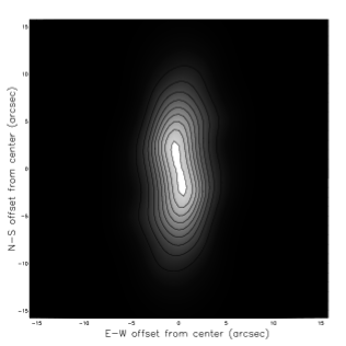
Figure 1: Spatial distribution of the surface brightness of the BL, interpolated from the values given by Vijh et al. (2005) using a TPS (see text for details). East is left, North is up, contour lines are in 5% intervals.

We were therefore able to integrate the TPS on the ISO apertures, to yield respectively $\sim{1.40\,\,10^{-17}}$ W cm^-2 for the $33^{\prime\prime}\times 20^{\prime\prime}$ rectangular aperture of SWS and $\sim{1.45\,\,10^{-17}}$ W cm^-2 for the circular aperture of diameter $84^{\prime\prime}$ of LWS. We remark that these integrated fluxes ought to be considered with caution, given the very sparse spatial sampling of the BL. Nonetheless, we used them to scale the calculated fluxes listed in tables 2, 4 and 5, which were computed for specific positions in the RR nebula, to these ISO apertures, for comparison with available ISO data. In particular, to estimate the fluxes expected to be observed by SWS using the $33^{\prime\prime}\times 20^{\prime\prime}$ aperture from the fluxes calculated for the RR lobe $2.5^{\prime\prime}$S $2.6^{\prime\prime}$E from the central source, we multiplied the latter by $\sim{1.40\,\,10^{-17}}$ W cm^-2 and divided the result by $\sim{4.58\,\,10^{-9}}$ W cm^-2 sr^-1 (the BL intensity measured by Vijh et al. (2005) at this position in the RR). To ease the comparison, Figs. 2 to 16 show the resulting scaled calculated spectra, along with the relevant spectra taken from the ISO data archive.

Figure 2: Comparison between the estimated IR emission spectrum of anthracene (C₁₄H₁₀) and an ISO spectrum of the RR in the wavelength range 2.5–4.0 $\mu$m. Calculated spectra, under different assumptions (see text for details), are drawn in dashed (calculated from the fluxes in second column of Table 2), dash–dotted (third column)

and continuous (fourth column) lines, the continuum–subtracted ISO spectrum is shown as a dotted line. The central positions of expected anthracene bands are marked by ticks.

Figure 3: Same as Fig. 2 in the wavelength range 5–15 $\mu$m.

Figure 4: Same as Fig. 2 in the wavelength range 13–30 $\mu$m.

Figure 5: Same as Fig. 2 in the wavelength range 25–45 $\mu$m.

Figure 6: Same as Fig. 2 in the wavelength range 100–120 $\mu$m.

Figure 7: Same as Fig. 2 for phenanthrene (C₁₄H₁₀) in the wavelength range 2.5–4.0 $\mu$m.

Figure 8: Same as Fig. 7 in the wavelength range 5–15 $\mu$m.

Figure 9: Same as Fig. 7 in the wavelength range 13–30 $\mu$m.

Figure 10: Same as Fig. 7 in the wavelength range 25–45 $\mu$m.

Figure 11: Same as Fig. 7 in the wavelength range 90–110 $\mu$m.

Figure 12: Same as Fig. 2 for pyrene (C₁₆H₁₀) in the wavelength range 2.5–4.0 $\mu$m.

Figure 13: Same as Fig. 12 in the wavelength range 5–15 $\mu$m.

For the SWS we chose the spectrum with the TDT number 70201801, a low–resolution full–grating scan. For the LWS we chose the spectrum with the TDT number 70901203, a medium resolution spectrum. In both cases, a cubic spline was fitted to the continuum below the emission bands, and subtracted before comparison. No further processing was performed on the ISO spectra, which therefore are by and large the automatically reduced spectra as obtained from the ISO data archive tool, just continuum–subtracted. In each figure we show the calculated IR emission bands from a given PAH, respectively scaled from the “high absorption rate” and “low absorption rate” $2.5^{\prime\prime}$S $2.6^{\prime\prime}$E columns (dashed and dash–dotted line), and scaled from the $2.5^{\prime\prime}$S $7.8^{\prime\prime}$E column (continuous line). The continuum–subtracted ISO spectrum is plotted as a dotted line. The positions of calculated bands are marked by ticks on each plot. Each expected band is plotted as a lorentzian curve (corresponding to homogeneous band broadening, see Pech et al. (2002)) whose integrated flux is normalised to the expected scaled value. The widths of the lorentzians were arbitrarily chosen to match those of the observed bands in the same spectral range. In particular, we used a FWHM of 0.024 $\mu$m for the in–plane C–H stretches around 3.3 $\mu$m, of 0.2 $\mu$m for bands between 6 and 15 $\mu$m, of 0.3 $\mu$m for bands between 15 and 25 $\mu$m, of 0.5 $\mu$m for bands between 25 and 50 $\mu$m and of 0.9 for bands longwards of 50 $\mu$m. These values are just an educated guess: many factors concur in determining the band shape and width for IR fluorescence bands of PAHs, such as lifetime broadening, anharmonicity, rotational structure. For a discussion of these effects see e. g. Pech et al. (2002). Such a detailed treatment would only be feasible, in principle, for those specific bands for which experimental measurements at different temperatures are available, i. e. not for the far–IR ones which appear to show the strongest diagnostic capability. Moreover it would be beyond the scope of the present work, since the precise band shape does not greatly affect its detectability.

Figure 14: Same as Fig. 12 in the wavelength range 13–30 $\mu$m.

Figure 15: Same as Fig. 12 in the wavelength range 25–45 $\mu$m.

Figure 16: Same as Fig. 12 in the wavelength range 90–110 $\mu$m.

We just remark that, on general grounds, bands which are mostly emitted when molecules are more highly excited are expected to be slightly redshifted due to anharmonicity (Joblin et al. 1995; Pech et al. 2002). As an example, we performed a detailed band shape calculation for the in–plane C–H stretch of pyrene, using the experimental data from Joblin et al. (1995). Figure 17 shows the result, which can be compared with Fig. 12 to see the impact of anharmonicity. Since the required experimental data are not currently available for phenanthrene and anthracene, we assumed for them the same anharmonicity parameters of pyrene. The resulting band profiles are shown in Figs. 18 and 19.

Considering the uncertainties in the calculated fluxes, anthracene appears to be compatible with all the ISO spectra, regardless of whether we use theoretical DFT band positions or the available gas phase positions measured by Cané et al. (1997) for the comparison with observations. The far–IR band at $\sim$110 $\mu$m might easily be hidden in the noise in the automatically reduced spectra available in the online ISO database. If anthracene alone were responsible for the whole observed BL emission, about two thirds of the total observed flux in the 3.3 $\mu$m band would be due to it as well. The slight position mismatch seen in Fig. 2 can be easily due to anharmonicity, as shown in Fig.  18. The band in the latter figure appears to be slightly too broad, but since we used the anharmonicity parameters of another molecule this is not definitive.

Figure 17: Comparison between the estimated IR emission spectrum of pyrene (C₁₆H₁₀) and an ISO spectrum of the RR in the wavelength range 2.5–4.0 $\mu$m, including detailed band–shape modelling. Calculated spectra, under different assumptions (see text for details), are drawn in dashed (calculated from the fluxes in second column of Table 5), dash–dotted (third column) and continuous (fourth column) lines, the continuum–subtracted ISO spectrum is shown as a dotted line. The central positions of fundamental pyrene bands are marked by ticks.

Phenanthrene, on the other hand, can possibly account at most for a small fraction of the observed BL: its rather strong quartet out–of–plane C–H bend at 13.6 $\mu$m and its skeletal bending mode at $\sim$100 $\mu$m are not apparently detected in the ISO spectra. The C–H bend was measured in vapour at $\sim$770 K to be at $\sim$13.7 $\mu$m (unpublished data from the measurements of Joblin (1992) and Joblin et al. (1994, 1995)). Moreover, if phenanthrene alone were responsible for the BL, it ought to produce more than twice the total observed flux in the 3.3 $\mu$m band. Even allowing for the fact that DFT calculations at the 4–31G level are known to somewhat overestimate the IR–activity of C–H modes (Langhoff 1996; Hudgins et al. 2001), this is still unrealistic. Finally, to account for the position mismatch between the predicted and observed band positions would require an anharmonicity band shift about an order of magnitude larger than the one obtained using the parameters of pyrene. Summing up, we conclude that fluorescence by neutral phenanthrene might contribute at most a small fraction of the observed BL.

Figure 18: Same as Fig. 17 for anthracene (C₁₄H₁₀).

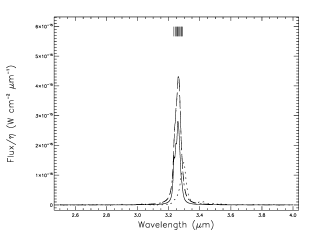
Figure 19: Same as Fig. 17 for phenanthrene (C₁₄H₁₀).

The case of pyrene is similar to that of phenanthrene, although slightly less clear–cut: it should also show a band at $\sim$100 $\mu$m which is undetected. This is one of the very few PAHs for which far–IR gas–phase measurements are available (Zhang et al. 1996), and the experimental band origin of this fundamental vibration lies at $\sim$105.3 $\mu$m, unfortunately in the most noisy part of the ISO LWS spectrum available online. The expected flux in this band would be sufficiently quenched by a high photon absorption rate to make it compatible with the observed spectrum, if pyrene were mainly concentrated in the lobes and relatively close to the central source. The expected out–of–plane C–H bend at $\sim$11.8 $\mu$m is a stronger constraint. This band was measured in vapour at $\sim$600 K to be at $\sim$11.9 $\mu$m (Joblin et al. 1994, 1995), and, as mentioned in the discussion for phenanthrene, DFT calculations at the 4–31G level are known to somewhat overestimate the IR–activity of C–H modes. Even allowing for all of these uncertainties, the expected band at $\sim$11.8 $\mu$m is at least a factor of $\sim$5 too strong to be compatible with the observed spectrum. As to the in–plane C–H stretch, if pyrene alone were responsible for the BL, it would produce all of the total observed flux in the 3.3 $\mu$m band. However, the band position we obtain even with a detailed band profile modelling which takes into account anharmonicity appears to be shifted bluewards of the observed peak. Summing up, we conclude that neutral pyrene might contribute at most $\sim$20% of the observed BL.

5 Discussion and conclusions

Vijh et al. (2004) and Vijh et al. (2005) put rather stringent limits on the plausible neutral PAHs as candidates for the BL in the RR: they restricted the range of possible candidates to molecules including from 3 to 4 aromatic rings. Among them, the only ones showing fluorescence spectral profiles compatible with the observed BL seem to be anthracene, phenanthrene and pyrene.

Upon a quick examination of the browsable online data from the ISO spectral database and comparison with our estimated IR fluxes, some bands stand out as the most promising diagnostics, due to their relatively high estimated intensities compared with ISO sensitivity: the out of plane C–H bends and the skeletal bending modes between $\sim$100 and $\sim$110 $\mu$m. In particular, even a cursory comparison between the estimated IR fluxes for phenanthrene and the available ISO SWS and LWS spectra show that its contribution to the production of the BL must be very small: indeed, fluorescence from phenanthrene would be so inefficient both in the lobes and in the halo of the RR that huge column densities would be needed to yield a significant contribution to the BL, and they would in turn also yield IR band intensities incompatible with observations. Phenanthrene and pyrene would produce prominent phosphorescence bands too, which have not been observed in the RR thus far (Witt 2005). All these elements, taken together, mean that only anthracene, among the three molecules considered, appears compatible with the observations.

Anthracene, if responsible for the BL, would also produce a quite substantial fraction of the observed flux in the in–plane C–H stretch bands. If it were to produce the observed BL, it would at the same time produce about half of the total observed flux at 3.3 $\mu$m. This is in good agreement with the observed spatial correlation between the latter band and the BL (Vijh et al. 2005).

However, we should also consider the bands which are absent from the calculated IR emission spectra: with the exception of the in–plane C–H stretch bands at 3.3 $\mu$m, all of the other classical aromatic bands, which are strong in the ISO data, are almost negligible in the calculated spectra for the three neutral PAHs considered here. If anthracene were responsible for the BL, then it would almost completely account for the observed flux in the 3.3 $\mu$m band; it follows that in this case the remaining aromatic bands must be produced by different carriers, which in turn must not contribute much flux to the 3.3 $\mu$m band. In particular, any mixture of neutral PAHs producing the observed flux in the out of plane C–H bends at $\sim$11.3 $\mu$m would also necessarily produce a substantial contribution to the 3.3 $\mu$m band, unless only large species, with more than $\sim$40 C atoms, are present. A possible solution may be to consider PAH cations, whose in–plane C–H stretch bands are well–known to be much less intense with respect to the same bands in their parent neutrals (see e. g. Langhoff 1996; Allamandola et al. 1999). This might account for the other strong bands observed in the RR, including the 11.3 $\mu$m band, which is not as reduced by ionisation.

This is consistent with observations by Bregman et al. (1993), which show the 3.3 and 11.3 $\mu$m bands to have very different spatial distributions, and would imply a scenario in which anthracene dominates the population of small neutral PAHs, producing both the 3.3 $\mu$m band and the BL and PAH cations produce the other aromatic bands, possibly with some contribution by large neutral PAHs for the 11.3 $\mu$m band. Some detailed modelling would be useful to determine whether such a scenario can be realistic and compatible with the photo–chemical evolution of PAHs in the RR environment.

The present data provide a powerful, quantitative diagnostic which may be used as a definitive cross–check for the hypothesis that small, neutral PAHs are responsible for the BL observed in the RR. Firm conclusions will require a thorough and careful review of available ISO spectroscopic data. In particular, all available LWS spectra in the 90–120 $\mu$m wavelength range ought to be appropriately reduced and stacked, to maximise the S/N ratio. The expected IR fluxes ought to be well within reach with the sensitivity of ISO observations, and will definitely be observable with forthcoming Herschel observations, which will go two orders of magnitude deeper (e. g. with the PACS instrument in the spectral range 57–210 $\mu$m, see the official PACS web page at http://pacs.ster.kuleuven.ac.be).

The accuracy of the IR emission spectra calculated in this paper would be greatly improved by a better understanding of the spatial distribution of PAH emission in the RR and, consequently, a better knowledge of the RF illuminating them. Indeed, the best available model of the RR (Men’shchikov et al. 2002) does not explicitly consider PAHs. Both more observational work, to better sample the spatial distribution of the BL as well as that of the IR emission, and more modelling are called for. In particular, observations of the BL with a much higher spatial resolution and sampling of the RR than those by Vijh et al. (2005) would be needed: this would enable us to adequately assess the dilution effect due to the large ISO SWS/LWS apertures without recurring to the extrapolations we used in Sect. 4.

We emphasize that experimental measurements of the precise position and intensities of all IR–active bands of anthracene, phenanthrene and pyrene in astrophysically relevant conditions would be very useful and reduce modelling errors: while the spectral range corresponding to “classical” AIBs has been well explored (see e. g. Joblin 1992; Szczepanski & Vala 1993; Joblin et al. 1994, 1995; Moutou et al. 1996; Cook et al. 1996; Hudgins et al. 1994; Hudgins & Allamandola 1995; Hudgins & Sandford 1998; Allamandola et al. 1999; Kim & Saykally 2002; Oomens et al. 2003), gas–phase measurements of far–IR bands of PAHs are sorely lacking to date. Last but not least, gas–phase measurements of the phosphorescence spectra of phenanthrene, pyrene and possibly other PAHs, which are also lacking to date, would provide yet another independent constraint amenable to direct observational verification of their presence in space.