Constraints on holographic dark energy from X-ray gas mass fraction of galaxy clusters

Abstract

We use the Chandra measurements of the X-ray gas mass fraction of 26 rich clusters released by Allen et al. to perform constraints on the holographic dark energy model. The constraints are consistent with those from other cosmological tests, especially with the results of a joint analysis of supernovae, cosmic microwave background, and large scale structure data. From this test, the holographic dark energy also tends to behave as a quintom-type dark energy.

Recent observations of Type Ia supernovae (SNe Ia) [1] indicate that the expansion of the Universe is accelerating at the present time. These results, when combined with the observations of cosmic microwave background (CMB) [2] and large scale structure (LSS) [3], strongly suggest that the Universe is spatially flat and dominated by an exotic component with large negative pressure, referred to as dark energy [4]. The first year result of the Wilkinson Microwave Anisotropy Probe (WMAP) shows that dark energy occupies about $73\%$ of the energy of our Universe, and dark matter about $23\%$. The usual baryon matter which can be described by our known particle theory occupies only about $4\%$ of the total energy of the Universe. Although we can affirm that the ultimate fate of the Universe is determined by the feature of dark energy, the nature of dark energy as well as its cosmological origin remain enigmatic at present. The most obvious theoretical candidate of dark energy is the cosmological constant $\Lambda$ which has the equation of state $w=-1$. An alternative proposal is the dynamical dark energy (quintessence) [5] which suggests that the energy form with negative pressure is provided by a scalar field evolving down a proper potential. The feature of this class of models is that the equation of state of dark energy $w$ evolves dynamically during the expansion of the Universe. However, as is well known, there are two difficulties arise from all these scenarios, namely the two dark energy (or cosmological constant) problems — the fine-tuning problem and the “cosmic coincidence” problem. The fine-tuning problem asks why the dark energy density today is so small compared to typical particle scales. The dark energy density is of order $10^{-47}{\rm GeV}^{4}$, which appears to require the introduction of a new mass scale 14 or so orders of magnitude smaller than the electroweak scale. The second difficulty, the cosmic coincidence problem, states “Since the energy densities of dark energy and dark matter scale so differently during the expansion of the Universe, why are they nearly equal today”? To get this coincidence, it appears that their ratio must be set to a specific, infinitesimal value in the very early Universe.

Recently, considerable interest has been stimulated in explaining the observed dark energy by the holographic dark energy model. For an effective field theory in a box of size $L$, with UV cut-off $\Lambda_{c}$ the entropy $S$ scales extensively, $S\sim L^{3}\Lambda_{c}^{3}$. However, the peculiar thermodynamics of black hole [6] has led Bekenstein to postulate that the maximum entropy in a box of volume $L^{3}$ behaves nonextensively, growing only as the area of the box, i.e. there is a so-called Bekenstein entropy bound, $S\leq S_{BH}\equiv\pi M_{p}^{2}L^{2}$. This nonextensive scaling suggests that quantum field theory breaks down in large volume. To reconcile this breakdown with the success of local quantum field theory in describing observed particle phenomenology, Cohen et al. [7] proposed a more restrictive bound – the energy bound. They pointed out that in quantum field theory a short distance (UV) cut-off is related to a long distance (IR) cut-off due to the limit set by forming a black hole. In other words, if the quantum zero-point energy density $\rho_{X}$ is relevant to a UV cut-off, the total energy of the whole system with size $L$ should not exceed the mass of a black hole of the same size, thus we have $L^{3}\rho_{X}\leq LM_{p}^{2}$. This means that the maximum entropy is in order of $S_{BH}^{3/4}$. When we take the whole Universe into account, the vacuum energy related to this holographic principle [8] is viewed as dark energy, usually dubbed holographic dark energy. The largest IR cut-off $L$ is chosen by saturating the inequality so that we get the holographic dark energy density

$$\rho_{X}=3c^{2}M_{p}^{2}L^{-2}~{},$$ (1)

where $c$ is a numerical constant, and $M_{p}\equiv 1/\sqrt{8\pi G}$ is the reduced Planck mass. If we take $L$ as the size of the current Universe, for instance the Hubble scale $H^{-1}$, then the dark energy density will be close to the observed data. However, Hsu [9] pointed out that this yields a wrong equation of state for dark energy. Li [10] subsequently proposed that the IR cut-off $L$ should be taken as the size of the future event horizon

$$R_{h}(a)=a\int_{t}^{\infty}{dt^{\prime}\over a(t^{\prime})}=a\int_{a}^{\infty}{da^{\prime}\over Ha^{\prime 2}}~{}.$$ (2)

Then the problem can be solved nicely and the holographic dark energy model can thus be constructed successfully. The holographic dark energy scenario may provide simultaneously natural solutions to both dark energy problems as demonstrated in Ref.[10]. For related work see [11, 12, 13, 14, 15, 16].

Consider now a spatially flat FRW (Friedmann-Robertson-Walker) Universe with matter component $\rho_{m}$ (including both baryon matter and cold dark matter) and holographic dark energy component $\rho_{X}$, the Friedmann equation reads

$$3M_{p}^{2}H^{2}=\rho_{m}+\rho_{X}~{},$$ (3)

or equivalently,

$${H^{2}\over H_{0}^{2}}=\Omega_{m}^{0}a^{-3}+\Omega_{X}{H^{2}\over H_{0}^{2}}~{}.$$ (4)

Note that we always assume spatial flatness throughout this paper as motivated by inflation. Combining the definition of the holographic dark energy (1) and the definition of the future event horizon (2), we derive

$$\int_{a}^{\infty}{d\ln a^{\prime}\over Ha^{\prime}}={c\over Ha\sqrt{\Omega_{X}}}~{}.$$ (5)

We notice that the Friedmann equation (4) implies

$${1\over Ha}=\sqrt{a(1-\Omega_{X})}{1\over H_{0}\sqrt{\Omega_{m}^{0}}}~{}.$$ (6)

Substituting (6) into (5), one obtains the following equation

$$\int_{x}^{\infty}e^{x^{\prime}/2}\sqrt{1-\Omega_{X}}dx^{\prime}=ce^{x/2}\sqrt{{1\over\Omega_{X}}-1}~{},$$ (7)

where $x=\ln a$. Then taking derivative with respect to $x$ in both sides of the above relation, we get easily the dynamics satisfied by the dark energy, i.e. the differential equation about the fractional density of dark energy,

$${d\Omega_{X}\over d\ln a}=\Omega_{X}(1-\Omega_{X})(1+{2\over c}\sqrt{\Omega_{X}})~{}.$$ (8)

This equation describes behavior of the holographic dark energy completely, and it can be solved exactly [10, 12]. From the energy conservation equation of the dark energy, the equation of state of the dark energy can be given [10]

$$w=-1-{1\over 3}{d\ln\rho_{X}\over d\ln a}=-{1\over 3}(1+{2\over c}\sqrt{\Omega_{X}})~{}.$$ (9)

Note that the formula $\rho_{X}={\Omega_{X}\over 1-\Omega_{X}}\rho_{m}^{0}a^{-3}$ and the differential equation of $\Omega_{X}$ (8) are used in the second equal sign. It can be seen clearly that the equation of state of the holographic dark energy evolves dynamically and satisfies $-(1+2/c)/3\leq w\leq-1/3$ due to $0\leq\Omega_{X}\leq 1$. In this sense, this model should be attributed to the class of dynamical dark energy models even though without quintessence scalar field. The parameter $c$ plays a significant role in this model. If one takes $c=1$, the behavior of the holographic dark energy will be more and more like a cosmological constant with the expansion of the Universe, and the ultimate fate of the Universe will be entering the de Sitter phase in the far future. As is shown in Ref.[10], if one puts the parameter $\Omega_{X}^{0}=0.73$ into (9), then a definite prediction of this model, $w_{0}=-0.903$, will be given. On the other hand, if $c<1$, the holographic dark energy will behave like a quintom-type dark energy proposed recently in Ref.[17], the amazing feature of which is that the equation of state of dark energy component $w$ crosses the phantom divide, $-1$, i.e. it is larger than $-1$ in the past while less than $-1$ near today. The recent fits to current SNe Ia data with parametrization of the equation of state of dark energy find that the quintom-type dark energy is mildly favored [18, 19]. Usually the quintom dark energy model is realized in terms of double scalar fields, one is a normal scalar field and the other is a phantom-type scalar field [20] (for quintom model see e.g. [21]). However, the holographic dark energy in the case $c<1$ provides us with a more natural realization for the quintom picture. If $c>1$, the equation of state of dark energy will be always larger than $-1$ such that the Universe avoids entering the de Sitter phase and the Big Rip phase. Hence, we see explicitly, the determination of the value of $c$ is a key point to the feature of the holographic dark energy as well as the ultimate fate of the Universe.

The holographic dark energy model has been tested and constrained by various astronomical observations [12, 13, 16]. In a recent work [16], it has been explicitly shown that regarding the latest supernova data as well as the CMB and LSS data, the holographic dark energy behaves like a quintom-type dark energy. This indicates that the numerical parameter $c$ in the model is less than 1. The best fit results provided by [16] are: $c=0.81$, $\Omega_{m}^{0}=0.28$, and $h=0.65$, which lead to the present equation of state of dark energy $w_{0}=-1.03$ and the deceleration/acceleration transition redshift $z_{T}=0.63$. It is necessary to test dark energy models and constrain their parameters using as many techniques as possible. Different tests might provide different constraints on the parameters of the model, and a comparison of results determined from different methods allows us to make consistency checks. In this Letter, we use the X-ray gas mass fraction of rich clusters, as a function of redshift, to constrain the holographic dark energy model, and to compare the results with the previous analysis.

The matter content of the largest clusters of galaxies is thought to provide an almost fair sample of the matter content of the Universe. A comparison of the gas mass fraction of galaxy clusters, $f_{\rm gas}=M_{\rm gas}/M_{\rm tot}$, inferred from X-ray observations, with $\Omega_{b}^{0}$ determined by nucleosynthesis can be used to constrain the density parameter of the Universe $\Omega_{m}^{0}$ directly [22]. Sasaki [23] and Pen [24] were the first to describe how the $f_{\rm gas}$ data of clusters of galaxies at different redshifts could also, in principle, be used to constrain the geometry and, therefore, dark energy relevant parameters of the Universe. The geometrical constraint arises from the fact that the measured $f_{\rm gas}$ values for each galaxy cluster depend on the assumed angular diameter distances to the clusters as $f_{\rm gas}\propto d_{A}^{3/2}$. The measured $f_{\rm gas}$ values should be invariant with redshift [23, 24, 25] when the reference cosmology used in making the measurements matches the true, underlying cosmology. The first successful application of such a test to constrain cosmological parameters was carried out by Allen et al. [26]; see also [27, 28, 29, 30, 31] and references herein. Note that the optically luminous galaxy (stellar) mass in clusters is about $0.19\sqrt{h}$ times the X-ray emitting gas mass, thus $\Omega_{b}^{0}=\Omega_{m}^{0}f_{\rm gas}(1+0.19\sqrt{h})$. In what follows we use the $f_{\rm gas}$ values, determined by Allen et al. [28] from Chandra observational data, to constrain the parameters of the holographic dark energy model. The redshifts of the 26 clusters range from 0.08 to 0.89.

Following [26, 27, 28, 29, 30, 31], we fit the $f_{\rm gas}$ data to the holographic dark energy model described by

$$f_{\rm gas}^{\rm mod}(z)={b\Omega_{b}^{0}\over(1+0.19\sqrt{h})\Omega_{m}^{0}}\left[{h\over 0.5}{d_{A}^{\rm SCDM}(z)\over d_{A}^{\rm mod}(z;\Omega_{m}^{0},c)}\right]^{3/2}~{},$$ (10)

where $d_{A}^{\rm mod}$ and $d_{A}^{\rm SCDM}$ are the angular diameter distances to the clusters in the current holographic model and reference SCDM cosmology, respectively, and $b$ is a bias factor motivated by gasdynamical simulations which suggest that the baryon fraction in clusters is slightly lower than for the Universe as a whole(see [27, 28] and references herein for detailed discussions). The angular diameter distances to the clusters are defined as

$$d_{A}=H_{0}^{-1}(1+z)^{-1}\int_{0}^{z}{dz^{\prime}\over E(z^{\prime})}~{},$$ (11)

where $H_{0}^{-1}$ (here we use the natural unit, namely the speed of light is defined to be 1) represents the Hubble distance with value $H_{0}^{-1}=2997.9h^{-1}$ Mpc, and $E(z)=H(z)/H_{0}$ can be obtained from (4), expressed as

$$E(z)=\left({\Omega_{m}^{0}(1+z)^{3}\over 1-\Omega_{X}}\right)^{1/2}~{}.$$ (12)

Note that for the holographic dark energy model the dynamical behavior of $\Omega_{X}$ is determined by (8); while for the SCDM model we have $\Omega_{X}=0$ and $\Omega_{m}^{0}=1$. It should be pointed out that the $f_{\rm gas}$ data used here are determined assuming an SCDM model with $h=0.5$. Hence there appears an $h/0.5$ factor in (10). We use the same Gaussian priors in our computation as [28, 30] with $h=0.72\pm 0.08$, $\Omega_{b}^{0}h^{2}=0.0214\pm 0.002$, and $b=0.824\pm 0.089$, all $1\sigma$ errors.

To constrain the parameters of the holographic dark energy model, we use a $\chi^{2}$ statistic

$$\chi^{2} = \sum_{i=1}^{26}{[f_{\rm gas}^{\rm mod}(z_{i};P)-f_{{\rm gas},i}]^{2}\over\sigma_{f_{\rm gas},i}^{2}}+\left({\Omega_{b}^{0}h^{2}-0.0214\over 0.002}\right)^{2}$$ (13)

$$+ \left({h-0.72\over 0.08}\right)^{2}+\left({b-0.824\over 0.089}\right)^{2}~{},$$

where $f_{\rm gas}^{\rm mod}(z_{i};P)$ is computed by the holographic dark energy model using (10), and $f_{{\rm gas},i}$ and $\sigma_{f_{\rm gas},i}$ are the measured value and error from [28] for a cluster at redshift $z_{i}$, respectively. The computation of $\chi^{2}$ is carried out in a five-dimensional space, for the five parameters $P=(\Omega_{m}^{0},c,h,\Omega_{b}^{0}h^{2},b)$. The probability distribution function (likelihood) of $\Omega_{m}^{0}$ and $c$ is determined by marginalizing over the “nuisance”parameters

$${\cal L}(\Omega_{m}^{0},c)=\int dhd(\Omega_{b}^{0}h^{2})db~{}e^{-\chi^{2}/2}~{},$$ (14)

where the integral is over a large enough range of $h$, $\Omega_{b}^{0}h^{2}$, and $b$ to include almost all the probability. We now compute ${\cal L}(\Omega_{m}^{0},c)$ on a two-dimensional grid spanned by $\Omega_{m}^{0}$ and $c$. The $68.3\%$, $95.4\%$, and $99.7\%$ (namely 1, 2, and 3 $\sigma$) confidence contours consist of points where the likelihood equals $e^{-2.31/2}$, $e^{-6.18/2}$, and $e^{-11.83/2}$ of the maximum value of the likelihood, respectively.

Figure 1: Confidence level contours of $68.3\%,~{}95.4\%$ and $99.7\%$ in the $(c,\Omega_{m}^{0})$ plane. The 1 $\sigma$ fit values for the parameters are: $\Omega_{m}^{0}=0.24^{+0.06}_{-0.05}$ and $c=0.61^{+0.45}_{-0.21}$, and the minimum value of $\chi^{2}$ in the five-dimensional parameter space is: $\chi_{\rm min}^{2}=25.00$.

Figure 1 shows our main results. We plot $68.3\%$, $95.4\%$, and $99.7\%$ confidence level contours in the $(c,\Omega_{m}^{0})$ plane. The best fit happens at $c=0.61$, $\Omega_{m}^{0}=0.24$, $h=0.73$, $\Omega_{b}^{0}h^{2}=0.0212$, and $b=0.812$, with $\chi_{\rm min}^{2}=25.00$. These results are in accordance with those obtained in [30] where some common results, $\Omega_{m}^{0}=0.24$ and $\chi^{2}_{\rm min}\sim 25$, were got from $f_{\rm gas}$ fits to three models — $\Lambda$CDM model, XCDM parametrization, and $\phi$CDM model (quintessence with power law potential). From Figure 1 we see clearly that the quality of the $f_{\rm gas}$ constraints is much better than that of the SNe Ia constraints (see Figure 2 of [16]), namely the contours are tighter than those derived from SNe Ia data. We find, however, that the $f_{\rm gas}$ constraints on the holographic model are consistent with those from a joint analysis of SNe Ia, CMB, and LSS data, but the constraints from the latter are tighter; see Figure 6 of [16] for comparison. The 1 $\sigma$ fit values for $c$ and $\Omega_{m}^{0}$ are: $c=0.61^{+0.45}_{-0.21}$ and $\Omega_{m}^{0}=0.24^{+0.06}_{-0.05}$. We notice that the fit value of $c$ is less than 1 in 1 $\sigma$ range, though it can be slightly larger than 1. This implies that according to the $f_{\rm gas}$ constraints the holographic dark energy basically behaves as a quintom-type dark energy in 1 $\sigma$ range.

Figure 2: Equation of state of dark energy $w$ and deceleration parameter $q$, versus red-shift $z$, from the best fit of the $f_{\rm gas}$ test.

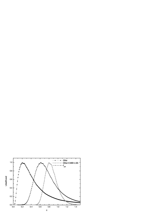
Figure 3: Likelihood distributions of parameter $c$ in the fits of SNe only, SNe+CMB+LSS, and $f_{\rm gas}$ data.

We now discuss about the cosmological consequences led by the best fit results of the $f_{\rm gas}$ data analysis. The evolutions of the equation of state of dark energy and the deceleration parameter of the Universe corresponding to the best fit are shown in Figure 2. From this figure, we see that the equation of state of dark energy $w$ has a value of $w_{0}=-1.29$ and the deceleration parameter $q$ has a value of $q_{0}=-0.97$ at present. The typical characteristic of the quintom-type dark energy is that the equation of state can cross $-1$. For this case, the crossing behavior $(w(z_{C})=-1)$ occurs at a redshift of $z_{C}=0.62$. In addition, the transition from deceleration to acceleration $(q(z_{T})=0)$ occurs at the redshift $z_{T}=0.70$. Comparing our plots in Figure 2 with the model-independent plots in [18], we find that the holographic plots for the $c=0.61$ case are in good agreement with those model-independent plots for the redshift range $z=0-2$. On the whole, the results derived from the $f_{\rm gas}$ constraints are consistent with those from other cosmological tests. The parameter $c$ which plays an important role in the holographic dark energy model is demonstrated to be less than 1 basically in 1 $\sigma$ range, which shows that the holographic dark energy tends to behave as quintom-type dark energy in the cosmological evolution. For comparing the probability distribution of the parameter $c$ determined by different cosmological tests, we show in Figure 3 the likelihood plots of $c$ corresponding to constraints from SNe, SNe+CMB+LSS ( for detail see [16]), and $f_{\rm gas}$ data, respectively, by furthermore marginalizing over the “nuisance” parameter $\Omega_{m}^{0}$. We see that the X-ray data provide a fairly good way for constraining the holographic dark energy.

In summary, we used in this Letter the recent X-ray cluster gas mass fraction data from the Chandra X-Ray Observatory to constrain the parameters of the holographic dark energy model. We considered a spatially flat FRW Universe with matter and holographic dark energy. For the holographic dark energy model, the numerical parameter $c$ plays a very important role in determining the evolutionary behavior of the space-time as well as the ultimate fate of the Universe. The constraints from the $f_{\rm gas}$ data show that in 1 $\sigma$ range the parameter $c$ is basically less than 1, which implies that the holographic dark energy tends to behave as a quintom-type dark energy. These constraints are consistent with those derived from other cosmological tests. The $f_{\rm gas}$ data are proven to be efficacious in constraining dark energy. We hope that the future $f_{\rm gas}$ data should provide an even tighter constraint on holographic dark energy model and other dark energy models.

- [1] A. G. Riess et al., Astron. J. 116 (1998) 1009 [astro-ph/9805201]; S. Perlmutter et al., Astrophys. J. 517 (1999) 565 [astro-ph/9812133].
- [2] C. L. Bennett et al., Astrophys. J. Suppl. 148 (2003) 1 [astro-ph/0302207]; D. N. Spergel et al., Astrophys. J. Suppl. 148 (2003) 175 [astro-ph/0302209].
- [3] M. Tegmark et al., Phys. Rev. D 69 (2004) 103501 [astro-ph/0310723]; M. Tegmark et al., Astrophys. J. 606 (2004) 702 [astro-ph/0310725].
- [4] S. Weinberg, Rev. Mod. Phys. 61 (1989) 1; S. M. Carroll, Living Rev. Rel. 4 (2001) 1 [astro-ph/0004075]; P. J. E. Peebles and B. Ratra, Rev. Mod. Phys. 75 (2003) 559 [astro-ph/0207347]; T. Padmanabhan, Phys. Rept. 380 (2003) 235 [hep-th/0212290].
- [5] C. Wetterich, Nucl. Phys. B 302 (1988) 668; P. J. E. Peebles and B. Ratra, Astrophys. J. 325 (1988) L17; R. R. Caldwell, R. Dave and P. J. Steinhardt, Phys. Rev. Lett. 80 (1998) 1582 [astro-ph/9708069]; I. Zlatev, L. Wang and P. J. Steinhardt, Phys. Rev. Lett. 82 (1999) 896 [astro-ph/9807002]; P. J. Steinhardt, L. Wang and I. Zlatev, Phys. Rev. D 59 (1999) 123504 [astro-ph/9812313].
- [6] J. D. Bekenstein, Phys. Rev. D 7 (1973) 2333; J. D. Bekenstein, Phys. Rev. D 9 (1974) 3292; J. D. Bekenstein, Phys. Rev. D 23 (1981) 287; J. D. Bekenstein, Phys. Rev. D 49 (1994) 1912; S. W. Hawking, Commun. Math. Phys. 43 (1975) 199; S. W. Hawking, Phys. Rev. D 13 (1976) 191.
- [7] A. G. Cohen, D. B. Kaplan and A. E. Nelson, Phys. Rev. Lett. 82 (1999) 4971 [hep-th/9803132].
- [8] G. ’t Hooft, gr-qc/9310026; L. Susskind, J. Math. Phys. 36 (1995) 6377 [hep-th/9409089].
- [9] S. D. H. Hsu, Phys. Lett. B 594 (2004) 13 [hep-th/0403052].
- [10] M. Li, Phys. Lett. B 603 (2004) 1 [hep-th/0403127].
- [11] K. Ke and M. Li, Phys. Lett. B 606 (2005) 173 [hep-th/0407056]; S. Hsu and A. Zee, hep-th/0406142;Y. Gong, Phys. Rev. D 70 (2004) 064029 [hep-th/0404030]; Y. S. Myung, Phys. Lett. B 610 (2005) 18 [hep-th/0412224]; Y. S. Myung, hep-th/0501023; H. Kim, H. W. Lee and Y. S. Myung, hep-th/0501118; Y. S. Myung, hep-th/0502128; Q. G. Huang and M. Li, JCAP 0408 (2004) 013 [astro-ph/0404229]; Q. G. Huang and M. Li, JCAP 0503 (2005) 001 [hep-th/0410095].
- [12] Q. G. Huang and Y. Gong, JCAP 0408 (2004) 006 [astro-ph/0403590]; Y. Gong, B. Wang and Y. Z. Zhang, Phys. Rev. D 72 (2005) 043510 [hep-th/0412218].
- [13] K. Enqvist and M. S. Sloth, Phys. Rev. Lett. 93 (2004) 221302 [hep-th/0406019]. K. Enqvist, S. Hannestad and M. S. Sloth, JCAP 0502 (2005) 004 [astro-ph/0409275]; H. C. Kao, W. L. Lee and F. L. Lin, Phys. Rev. D 71 (2005) 123518 [astro-ph/0501487]; J. Shen, B. Wang, E. Abdalla and R. K. Su, hep-th/0412227.
- [14] E. Elizalde, S. Nojiri, S. D. Odintsov and P. Wang, Phys. Rev. D 71 (2005) 103504 [hep-th/0502082]; B. Wang, Y. Gong, and E. Abdalla, hep-th/0506069; B. Wang, C.-Y. Lin, and E. Abdalla, hep-th/0509107; H. Kim, H. W. Lee, and Y. S. Myung, gr-qc/0509040.
- [15] X. Zhang, Int. J. Mod. Phys. D 14 (2005) 1597 [astro-ph/0504586].
- [16] X. Zhang and F.-Q. Wu, Phys. Rev. D 72 (2005) 043524 [astro-ph/0506310].
- [17] B. Feng, X. Wang and X. Zhang, Phys. Lett. B 607 (2005) 35 [astro-ph/0404224].
- [18] U. Alam, V. Sahni, and A. A. Starobinsky, JCAP 0406 (2004) 008 [astro-ph/0403687].
- [19] D. Huterer and A. Cooray, Phys. Rev. D 71 (2005) 023506 [astro-ph/0404062].
- [20] Z. Guo, Y.-S. Piao, X. Zhang and Y. Zhang, Phys. Lett. B 608 (2005) 177 [astro-ph/0410654].
- [21] B. Feng, M. Li, Y.-S. Piao, and X. Zhang, astro-ph/0407432; H. Wei, R.-G. Cai, and D.-F. Zeng, Class. Quant. Grav. 22 (2005) 3189 [hep-th/0501160]; G.-B. Zhao, J.-Q. Xia, M. Li, B. Feng, and X. Zhang, astro-ph/0507482; H. Wei, and R.-G. Cai, astro-ph/0509328.
- [22] S. D. M. White and C. S. Frenk, Astrophys. J. 379 (1991) 52; A. C. Fabian, Mon. Not. Roy. Astron. Soc. 253 (1991) L29; S. D. M. White, J. F. Navarro, A. E. Evrard, and C. S. Frenk, Nature 366 (1993) 429; S. D. M. White and A. C. Fabian, Mon. Not. Roy. Astron. Soc. 273 (1995) 72; A. E. Evrard, Mon. Not. Roy. Astron. Soc. 292 (1997) 289 [astro-ph/9701148]; M. Fukugita, C. J. Hogan, and P. J. E. Peebles, Astrophys. J. 503 (1998) 518 [astro-ph/9712020]; S. Ettori and A. C. Fabian, Mon. Not. Roy. Astron. Soc. 305 (1999) 834 [astro-ph/9901304].
- [23] S. Sasaki, Publ. Astron. Soc. Jap. 48 (1996) L119 [astro-ph/9611033].
- [24] U. Pen, New Astron. 2 (1997) 309 [astro-ph/9610090].
- [25] V. R. Eke, J. F. Navarro and C. S. Frenk, Astrophys. J. 503 (1998) 569 [astro-ph/9708070].
- [26] S. W. Allen, R. W. Schmidt, and A. C. Fabian, Mon. Not. Roy. Astron. Soc. 334 (2002) L11 [astro-ph/0205007].
- [27] S. W. Allen, R. W. Schmidt, A. C. Fabian, and H. Ebeling, Mon. Not. Roy. Astron. Soc. 342 (2003) 287 [astro-ph/0208394].
- [28] S. W. Allen, R. W. Schmidt, H. Ebeling, A. C. Fabian, and van Speybroeck, Mon. Not. Roy. Astron. Soc. 353 (2004) 457 [astro-ph/0405340].
- [29] J. A. S. Lima, J. V. Cunha and J. S. Alcaniz, Phys. Rev. D 68 (2003) 023510 [astro-ph/0303388].
- [30] G. Chen and B. Ratra, Astrophys. J. 612 (2004) L1 [astro-ph/0405636].
- [31] Z.-H. Zhu, M.-K. Fujimoto and X.-T. He, Astron. Astrophys. 417 (2004) 833 [astro-ph/0401095]; Z.-H. Zhu, M.-K. Fujimoto and X.-T. He, Astrophys. J. 603 (2004) 365 [astro-ph/0403228]; Z.-H. Zhu, Astron. Astrophys. 423 (2004) 421 [astro-ph/0411039].