A Cosmic Relation between Extinction and Star Formation

Abstract

We study the relation between the star formation intensity of galaxies and the extinction by dust of their emitted light. We employ a detailed statistical analysis of Hubble Deep Field North data to show a clear positive correlation between the extinction and star formation intensity at all epochs from redshift 0.4 to 6.5. The extinction evidently increases with time for a given star formation intensity, consistent with the expected increase in the metallicity with time. Our observational results are well fitted at all epochs by a double power-law model with a fixed shape that simply shifts with redshift. The correlation between the extinction and the star formation intensity can be interpreted by combining two other trends: the correlation between the star formation rate and the gas content of galaxies, and the evolution of the dust-to-gas ratio in galaxies. If we assume that Kennicutt’s observed relation for the former is valid at each redshift, then our findings imply an interesting variation in the dust-to-gas ratio in galaxies within each epoch and with time, and suggest new ways to investigate the cosmic evolution of this quantity.

1 Introduction

In this Letter we investigate the relation between the extinction and the star formation rate (SFR) in galaxies at various epochs. Understanding this relation is a key for better understanding the physical conditions in the interstellar medium (ISM) of galaxies as well as the environments of galaxies and their cosmic evolution. The SFR in galaxies has been studied extensively in recent years. The most widely used star formation law, originally conjectured by Schmidt (1959), correlates the SFR in galaxies and their gas density as a power law. As summarized and integrated by Kennicutt (1998), many empirical studies have tested and proven the effectiveness of the Schmidt law. Now, extinction by dust is related to star formation since dust forms from heavy elements ejected during stellar mass loss. Also, the dust-to-gas ratio is related to the metallicity of the interstellar gas (Schmidt & Boller, 1993; Kim & Martin, 1996).

It is thus clear that a correlation should exist between the SFR and the extinction. Indeed, previous observations indicate such a correlation within galaxies, and for galaxies at various redshifts [e.g., Adelberger & Steidel (2000); Calzetti (2001); Calzetti et al. (2005)]. The goal of this paper is to observe this correlation and determine its form for a broad range of redshifts, and to demonstrate that our conclusions are not strongly affected by selection effects. In the following section we describe the dataset used for the analyses in this Letter. In section 3 we test the dataset to verify that it is statistically valid and can be used for the analyses to follow. We present our main results and model fits in sections 4 and 5, and give our conclusions in section 6. We note that we focus on the correlation of extinction with the star formation intensity (SFI) of galaxies (which is the SFR per unit area), but consider in § 5 also the correlation with the total SFR.

2 The Data

We used the dataset described in detail in Thompson, Waymann & Storrie-Lombardi (2001; hereafter TWS) and Thompson (2003). It is a combination of observations of the Hubble Deep Field North (HDF-N) with the Wide Field Planetary Camera 2 [WFPC 2; Williams et al. (1996)] and with the Near-Infrared Camera and Multi-Object Spectrometer [NICMOS; Dickinson (2000)). The main output of the photometric analysis in TWS and Thompson (2003) was the most likely combination of redshift, extinction and spectral energy distribution (SED) for each of the galaxies that passed the selection criteria. However, in this present work we utilized not only the most likely combinations but the entire database of the photometric analysis. The idea is that while the uncertainties are large from each photometric fit to an individual galaxy, if we include these uncertainties properly then the total dataset of thousands of galaxies will have strong statistical power for studying galaxy evolution.

The dataset includes two three-dimensional matrices for each of the 1972 galaxies that passed the selection criteria and were used for the analysis. The matrix dimensions are $101\times 51\times 15$, corresponding to 101 possible redshift values between 0 and 8, 15 extinction values ranging from $E(B-V)=0$ to 1.0, and 51 possible SED templates. The first matrix holds the $\chi^{2}$ values for each of the redshift, extinction and SED template combinations, determined as described in TWS by computing the goodness-of-fit to the six observed photometric fluxes. Note that in computing the $\chi^{2}$, TWS added a term to the background noise that is $10\%$ of the flux, to represent various systematic effects. As discussed further in TWS, this term may overestimate the noise somewhat and lead to an underestimate of the $\chi^{2}$ values, producing in our analysis below a slightly broader distribution of probable parameter values. The second matrix in the dataset holds the UV flux at 1500Å rest-frame that corresponds to each of the redshift, extinction and template combinations. We used this matrix to determine the SFR that corresponds to the different combinations according to the broadband 1500Å relation given by Madau, Pozzetti, & Dickinson (1998), modified for a Scalo (1998) IMF:

$$F_{1500}=10.0\times 10^{27}\ {\rm SFR}\left[M_{\odot}{\rm yr}^{-1}\right]\ {\rm erg\,s^{-1}\,Hz}^{-1}\ .$$ (1)

In addition to the above photometric dataset, for 131 galaxies spectroscopic redshifts are available from Cohen (2001). For these galaxies, we adopted the spectroscopic redshift and used the above matrices to determine the likelihood of various extinctions and SED templates given the known redshift.

3 Testing the Dataset using Redshift Error Analysis

In general, a $\chi^{2}$ value is related to the corresponding probability through the relation:

$$P\propto\exp\left(-\frac{1}{2}\chi^{2}\right)\ .$$ (2)

We therefore used this relation to convert, for each galaxy, the $\chi^{2}$ values that correspond to the different combinations of redshift, extinction and template, into their corresponding probabilities. The combinations for each galaxy were then divided into two groups, one with redshift values higher than the redshift value of the most probable combination, and the other with redshift values that are lower than the redshift value of the most probable combination. We then found 1-$\sigma$ redshift confidence limits upwards and downwards by identifying the redshift values at 0.683 of the cumulative probability of each of the two groups. We emphasize that a full probability distribution of possible parameters is determined by fitting to each observed galaxy. Figure 1 compares the photometric redshift values with errors to the spectroscopic values for the 131 galaxies for which spectroscopic data are available from Cohen (2001). This plot is similar to the plot in figure 3 in Thompson (2003) with the significant difference that here the 1-$\sigma$ confidence limits take into account the entire distribution of possible photometric redshifts, a distribution that in some cases is very wide or multiply-peaked.

Figure 1: Photometric redshift versus spectroscopic redshift for each galaxy (in a log plot of $1+z$). The confidence limits of 1-$\sigma$ up and 1-$\sigma$ down for the photometric redshifts were determined using the probability distribution of the photometric redshift of each galaxy. The spectroscopic data are taken from Cohen (2001)

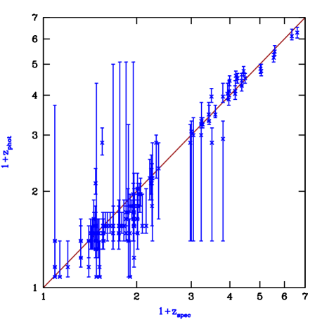
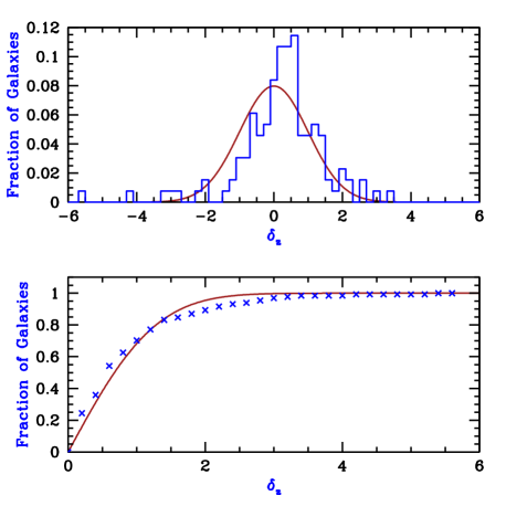
The photometric redshifts and their calculated errors, together with the spectroscopic redshift data, can be used to test the validity of the photometric analysis dataset. This test is important as the analysis in the following sections strongly relies on the statistical properties of the $\chi^{2}$ matrices. The photometric redshifts deviate from the spectroscopic ones, but we now consider how these deviations are distributed. If the statistical analysis is valid, then the distribution of the deviations between the photometric and the spectroscopic redshift should be roughly Gaussian, with standard deviation as predicted by the statistical analysis. Rather than restricting to a symmetric distribution, we apply the separately-determined upper and lower confidence limits. Figure 2 shows the normalized relative redshift error distribution (upper panel). We define $\delta_{z}$ as the fractional redshift error expressed in standard deviations:

$$\delta_{z}\equiv\frac{|z_{\rm spec}-z_{\rm phot}|}{\sigma_{\pm}}\ ,$$ (3)

where $\sigma_{\pm}$ is the upper or lower confidence limit which is chosen according to whether the spectroscopic redshift is higher or lower than the photometric one, respectively. In the Figure we also show (lower panel) the cumulative distribution of all the points, both those with positive and those with negative errors. We find that the empirical distribution is indeed close to a normal distribution with a standard deviation that agrees well with that predicted by our fitting method; in particular, the cumulative 1-$\sigma$, 2-$\sigma$ and 3-$\sigma$ values are 0.702, 0.893 and 0.969, compared to the theoretical expectation of 0.683, 0.954, and 0.997, respectively.

Figure 2: Upper panel: The normalized distribution of the fractional redshift error expressed in standard deviations, $\delta_{z}$, defined in equation (3). Lower panel: The cumulative distribution of $\delta_{z}$. The solid curves in the two panels represent the theoretical Gaussian and error function curves, respectively.

4 Correlating the Extinction with the Star Formation Intensity

The SFI (denoted $x$) is defined as the SFR per area, expressed in solar mass per year per proper kiloparsec squared. As described in section 2, various combinations of redshift, extinction and template may be associated with each galaxy and for each of these combinations the SFI can be determined. First the SFR of each combination is determined from equation (1), and then the area is calculated (for each possible redshift) from the number of pixels that the galaxy covers in the HDF-N image. The average SFI of the galaxy is then the SFR divided by the proper area. We emphasize that in the analysis below we use the average extinction and SFI of each galaxy, and do not consider individual pixels separately. In this work we assume in all cosmological conversions a flat cosmology with $h=0.72$, $\Omega_{m}=0.27$ and $\Omega_{\Lambda}=0.73$.

We now consider our main objective in this Letter which is to correlate the extinction and the SFI. As noted in section 3, the probabilities of the different combinations of extinction, redshift and template for each galaxy can be calculated using the $\chi^{2}$ values associated with the combinations together with equation (2). Having obtained the probabilities, for each galaxy we statistically sample this distribution 200 times in a Monte Carlo approach. The data that are used in the following analysis are the redshift, extinction and the calculated SFI values, for each of the 200 sample combinations, for each of the 1927 galaxies used in this Letter. This Monte-Carlo approach includes statistically all the uncertainties and degeneracies from the photometric fits of the individual galaxies. Figure 3 (upper panel) plots the extinction versus $x$ for combinations with redshifts $z=0.7$–1.0. The binning of the extinction values is apparent. There are 12,072 points in the plot and their distribution clearly points to a correlation between the extinction and the SFI.

Figure 3: Upper panel: Plot of the extinction $E(B-V)$ versus $x$ for the redshift bin $z=0.7$–1.0. The detection threshold is apparent as a linear cutoff at the upper-left end of the distribution of data points (i.e., at low $x$ or high $E(B-V)$ values). Lower panel: Histogram of the $x$ values in the upper panel that correspond to $E(B-V)=0.2$. Note that the peak lies far from the detection limit.

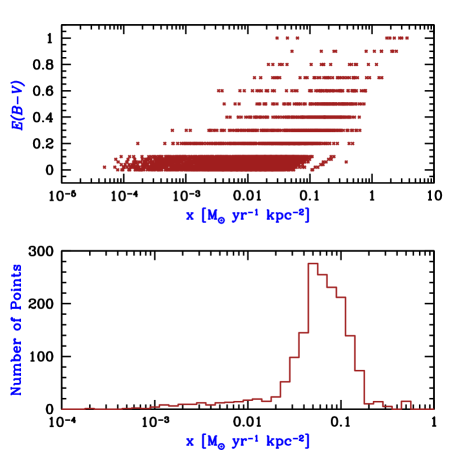
We note that some caution is needed here, since a correlation between the extinction and the SFI would have been introduced into our analysis simply as a selection effect; thus we must carefully demonstrate that the observed correlation is instead a real effect. To identify an object as a galaxy, the selection procedure (as described in TWS) requires a minimum flux per pixel in the various filter wavebands. At any given redshift, objects with very low x values or with high extinction values may exist and not be detected. This selection effect is evident in the upper panel of Figure 3 as a lack of galaxies at the low $x$ and high $E$ region (i.e., the top-left corner). More specifically, the left boundary of the collection of data points is quite linear (as is the case in other redshift bins as well). Since the detectability of galaxies is roughly set by a minimum surface brightness, and the observed surface brightness is proportional to the intrinsic $x$ of the galaxy times an extinction correction of the form $\exp[-aE(B-V)]$ for some constant $a$, then galaxies with observed flux at the detection limit should lie on a straight line in $E$ versus $\log_{10}(x)$.

In general, a correlation between the extinction and the SFI could be inferred mistakenly due to this selection effect, but in Figure 3 this is not the case. The selection effect is relevant only at low $x$ and high $E$, but figure (3a) also shows a clear lack of points at high $x$ and low $E$, where any galaxies would be easily detected, and selection effects are absent.

To demonstrate this more clearly, the data points at each extinction value were tested to verify that most of the $x$ values lie far above the detection limit, and thus the mean $x$ value (which we use below) is insensitive to selection effects. The lower panel of Figure 3 shows a histogram of the $\log_{10}(x)$ values that correspond to $E(B-V)=0.2$ in the upper panel of the same figure. As can be seen, the detection limit in this case is around $\log_{10}(x)=-3$, whereas most of the data points lie at $\log_{10}(x)=-1.6$ or higher, and the average is at -1.1. This behaviour, which we have verified for other extinction values and other redshift bins, clearly indicates that the selection effect is not the main cause of the correlation we find between the extinction and SFI. We caution though that at the highest redshifts we consider, there are fewer observed galaxies and fewer data points particularly at high extinction, so the detection threshold affects the results significantly in this regime. Additional data at fainter fluxes would be very useful for checking the reliability of the high-redshift, high-extinction points.

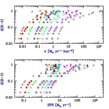
In order to characterize the correlation between the extinction and the SFI as a function of epoch, we divided the data into ten redshift bins: 0.4–0.7, 0.7–1.0, 1.0–1.5, 1.5–2.0, 2.0–2.5, 2.5–3.0, 3.0–3.5, 3.5–4.5, 4.5–5.5 and 5.5–6.5. In each redshift bin, the mean and standard deviation of all the $\log_{10}(x)$ values that correspond to each specific extinction value were calculated. We calculated symmetric errors here in order to use them below in a $\chi^{2}$ minimization. The resulting extinction and mean $\log_{10}(x)$ values, with 1-$\sigma$ error bars in $\log_{10}(x)$, are plotted in Figure 4 for all redshift bins. The correlation between the extinction and SFI is clearly evident at all epochs. Note that the errors in $x$ [which is proportional to $(1+z)^{4}$] are smaller in the higher-redshift bins since the photometric redshifts are more accurate due to the Lyman break (see also figure 1).

Figure 4: Plots of the extinction $E(B-V)$ versus the SFI at various redshift bins between $z=0.4$ and 6.5. The correlation between the extinction and the SFI is clearly observed at all these epochs. We show the double power-law fit to the data (solid curves). We also compare to a power-law slope of 0.71 (dashed curve, $z=0.7$–1.0 panel). See section 5 for a discussion of the model fits

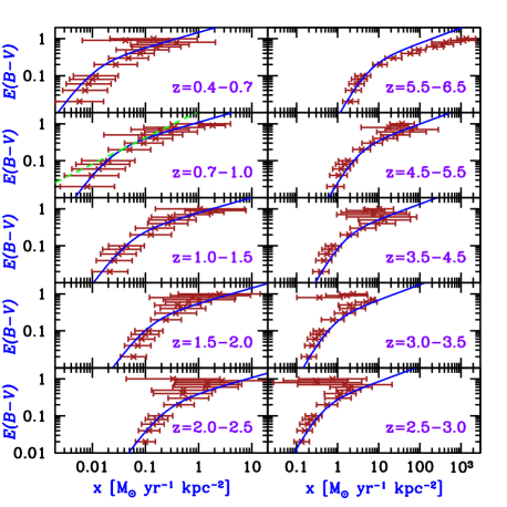
Figure 5 (upper panel) plots all the redshift bins together so that the evolution with redshift can be observed more easily. It is evident that for a given SFI, the extinction decreases with $z$. This behaviour is consistent with the increase in the metallicity of the ISM with time (Inoue, 2003). The lower panel of Figure 5 is similar and is based on the same analysis as the upper panel except that the extinction is plotted against the total SFR and not against the SFI. Although the results in the lower panel depend differently on the size distribution of galaxies, the same behaviour is seen as in the upper panel. We further consider these two different correlations in the following section.

Figure 5: Plot of $E(B-V)$ versus $x$ (upper panel) or versus the SFR (lower panel) for all redshift bins. The bins are $z=0.4$–0.7 ($\times$), 0.7–1.0 ($\bullet$), 1.0–1.5 ($\star$), 1.5–2.0 (open squares), 2.0–2.5 (+), 2.5–3.0 (solid triangles), 3.0–3.5 ($\circ$), 3.5–4.5 (solid squares), 4.5–5.5 ($\diamond$) and 5.5–6.5 (open triangles).

5 Fitting the Correlation

In the previous section, the relation between the extinction and SFI was described empirically. As noted in the introduction, this relation is expected from the Schmidt law together with the correlation between the gas and dust in the ISM of galaxies.

Schmidt (1959) put forth the hypothesis that the rate of star formation in a given region varies as a power of the gas density within that region. Observations yield direct estimates of surface densities and thus, the relation between the SFI $x$ and the gas surface density has been measured over a broad range of physical conditions in relatively nearby galaxies, yielding the relation $x\propto\Sigma_{\rm gas}^{1.4}$ (Kennicutt, 1998). The relation between the dust and gas content in the ISM is less clear. If a constant dust-to-gas ratio is assumed, then if the Kennicutt relation is valid at a given redshift it should yield a linear relation between $x$ and $E$, with a slope of $1/1.4=0.71$ in a log-log scale. However, this model is inconsistent with the observational results shown in Figure 4. To illustrate this, we show in the top-right panel ($z=0.7$–1) of this figure a line with this slope (dashed curve). It is apparent in all the redshift bins that the dependence of $E$ on $x$ in the actual data is steeper than this power at low $x$ and shallower at high $x$. Equivalently, the dust-to-gas ratio at both ends is lower than at the central $x$ values, assuming the Kennicutt (1998) relation is valid at each redshift.

The behaviour in Figure 4 suggests a double power-law model; the precise form we choose is motivated by the conventional model for the luminosity function of quasars [e.g., Peterson (1997)]. In addition, Figure 5 suggests a simple evolution with redshift as a power of $(1+z)$, and so we fit a single model to all epochs simultaneously:

$$E(B-V)=\frac{E_{0}(1+z)^{\gamma_{1}}}{\left[\frac{x}{x_{S}(1+z)^{\gamma_{2}}}\right]^{-\alpha}+\left[\frac{x}{x_{S}(1+z)^{\gamma_{2}}}\right]^{-\beta}}\ .$$ (4)

This model consists of six free parameters: $E_{0}$ – a normalization parameter, $x_{S}$ – the knee point that separates the two slopes, $\gamma_{1}$ and $\gamma_{2}$ – the powers of $(1+z)$ that describe the redshift evolution of $E_{0}$ and $x_{S}$, respectively, and $\alpha$ and $\beta$, which represent the asymptotic power-law slopes at low and high $x$-values, respectively. Note that we excluded $E=0$ data points from the fit and from Figures 4 and 5.

We fit the model to all redshift bins by minimizing a combined $\chi^{2}$ built according to the errors shown in Figure 4. The figure shows that the model yields a rather good fit to the data at all epochs. The redshift value of the fit shown in each panel is the value at the center of the redshift bin. The fitted parameters with their 1-$\sigma$ errors (which correspond to a unit increase in the $\chi^{2}$ value from its minimum value) are: $\log_{10}(E_{0})=-0.65^{+.23}_{-.21}$, $\log_{10}(x_{S})=-2.79^{+.19}_{-.23}$, $\gamma_{1}=0^{+.03}_{-.04}$, $\gamma_{2}=4.14^{+.12}_{-.13}$, $\alpha=2.03^{+.71}_{-.42}$, and $\beta=0.41^{+.11}_{-.13}$.

The best-fit value $\gamma_{1}=0$ implies a relation of constant shape that simply shifts horizontally with redshift. The $\chi^{2}$ value of the best fit is 111.6 while the number of degrees of freedom is 134, which suggests that the errors may be somewhat overestimated, which is perhaps related to our assuming uncorrelated errors for the various points when constructing the $\chi^{2}$ for this fit. Figure 5 reveals another possible characterization of the correlation by relating the extinction to the SFR instead to the SFI. The double power law was fitted to these data as well, using the same analysis as described above for the case of the SFI. The fitted parameter results in this case, with a best-fit $\chi^{2}$ value of 107.1, are: $\log_{10}(E_{0})=-0.39^{+.08}_{-.07}$, $\log_{10}(x_{S})=-0.62^{+.14}_{-.13}$, $\gamma_{1}=0^{+.08}_{-.53}$, $\gamma_{2}=2.16^{+.21}_{-.20}$, $\alpha=2.17^{+.42}_{-.3}$, and $\beta=0.22^{+.05}_{-.06}$.

The two fits presented here depend on the sizes of galaxies in different ways. While the SFI is a more local quantity, the total SFR depends also on the global size of the galaxy. A galaxy’s overall size and mass affects star formation through global feedback effects. In particular, supernova feedback is efficient only in relatively small galaxies which results in various observed correlations in the properties of galaxies at low redshift [e.g., Dekel & Birnboim (2005)]. Additional data for a larger number of galaxies is required to fully explore the effect of the size of a galaxy on its average extinction value.

6 Conclusions

We have shown that a clear correlation exists between the extinction of galaxies and their SFI. This correlation is apparent at various epochs ranging from z=0.4 to z=6.5 and is in general agreement with an increasing metallicity in the ISM with time. We have also shown that a similar correlation remains when the galaxies’ SFR is considered instead of their SFI, a case in which global effects such as supernovae feedback may affect the behaviour. We have fitted a double power-law model to the results and shown that it fits the data well. We have suggested that this correlation is a natural consequence of the Schmidt law, which relates the SFI of galaxies with their gas content in the ISM, together with a relation that exists between the gas and dust content in the ISM. The exact shape of the correlation should be further investigated both to further eliminate selection effects and to shed more light on the cosmic evolution of gas and dust in galaxies.

References

- Adelberger & Steidel (2000) Adelberger K. L., Steidel C. C., 2000, ApJ, 544, 218
- Calzetti (2001) Calzetti D., 2001, PASP, 113, 1449
- Calzetti et al. (2005) Calzetti D., et al., 2005, ApJ, 633, 871
- Cohen (2001) Cohen, J. G. 2001, AJ, 121, 2895
- Dekel & Birnboim (2005) Dekel, A., & Birnboim, Y. 2005, preprint (astro-ph/0412300)
- Dickinson (2000) Dickinson, M. 2000, Philos. Trans. R. Soc. London, A, 358, 2001
- Inoue (2003) Inoue, A. K. 2003, PASJ, 55, 901
- Kennicutt (1998) Kennicutt, R. C., Jr. 1998 ApJ, 498, 541
- Kim & Martin (1996) Kim, S., & Martin, P. G. 1996, ApJ, 462, 296
- Madau, Pozzetti, & Dickinson (1998) Madau, P., Pozzetti, L., Dickinson, M. 1998, ApJ, 559, 620
- Peterson (1997) Peterson, B. M. 1997, An Introduction to Active Galactic Nuclei, Cambridge Univ. Press, Cambridge
- Scalo (1998) Scalo, J. 1998, in ASP conference series Vol 142, The Stellar Initial Mass Function, eds. G. Gilmore & D. Howell, p. 201 (San Francisco: ASP)
- Schmidt (1959) Schmidt, M. 1959, ApJ, 129, 243
- Schmidt & Boller (1993) Schmidt, K.-H., & Boller, T. 1993, Astron. Nachr., 314, 361
- (15) Thompson, R. I., Waymann, R. J. & Storrie-Lombardi, L. J. 2001, ApJ, 546, 694 (TWS)
- Thompson (2003) Thompson, R. I. 2003, ApJ, 596, 748
- Williams et al. (1996) Williams, R. E., et al. 1996, AJ, 112, 1335