Properties of O VI Absorption in the Local Interstellar Medium

Abstract

The measurement of absorption over short distances in the local interstellar medium (LISM) provides an excellent opportunity to study the properties of O VI absorption and its kinematic relationship to absorption by tracers of cool and warm gas. We report on the properties of LISM O VI absorption observed with 20 ${\rm km\,s}^{-1}$  resolution Far Ultraviolet Spectroscopic Explorer (FUSE)  observations of 39 white dwarfs (WDs) ranging in distance from 37 to 230 pc with a median distance of 109 pc. LISM O VI is detected with $\geq 2\sigma$ significance along 24 of 39 lines of sight. The column densities range from $\log N($O VI$)=12.38$ to 13.60 with a median value of 13.10. The line of sight volume density, $n($O VI$)=N($O VI$)/d$, exhibits a large dispersion ranging from (0.68 to $13.0)\times 10^{-8}$ cm^-3 with an average value $n($O VI$)=3.6\times 10^{-8}$ cm^-3 twice larger than found for more distant sight lines in the Galactic disk. The Doppler parameter, $b$, for the $\geq 4\sigma$ O VI detections range from $15.0\pm 3.5$ to $36.2\pm 7.3$ ${\rm km\,s}^{-1}$, with average and dispersion of $23.0\pm 5.6$ ${\rm km\,s}^{-1}$. The narrowest profiles are consistent with thermal Doppler broadening of O VI near its temperature of peak abundance, $2.8\times 10^{5}$ K. $\log N($O VI) is observed to correlate with $b$. The broader profiles are tracing a combination of O VI with $T>2.8\times 10^{5}$ K, multiple component O VI absorption either in interfaces or hot bubbles, and/or the evaporative outflow of conductive interface gas. Comparison of the average velocities of O VI and C II absorption reveals 10 cases where the O VI absorption is closely aligned with the C II absorption as expected if the O VI is formed in a condensing interface between the cool and warm absorption traced by C II (and also O I and C III) and a hot exterior gas. The comparison also reveals 13 cases where O VI absorption is displaced to positive velocity by 7 to 29 ${\rm km\,s}^{-1}$ from the average velocity of C II. The positive velocity O VI is mostly found in the north Galactic hemisphere. The positive velocity O VI appears to be tracing the evaporative flow of O VI from a young interface between warm gas and a hot exterior medium. However, it is possible the positive velocity O VI is instead tracing cooling hot Local Bubble (LB) gas. The properties of the O VI absorption in the LISM are broadly consistent with the expectations of the theory of conductive interfaces caught in the old condensing phase and possibly in the young evaporative phase of their evolution.

1 Introduction

An important source of information about hot gas in interstellar space is the lithium-like O VI ion with doublet transitions in the far-ultraviolet at 1031.93 and 1037.62 Å. The conversion of O V into O VI requires 113.9 eV. Since normal hot stars rarely have large radiative fluxes at energies exceeding the He⁺ absorption edge at 54.4 eV, the O VI found in the interstellar medium is most likely created by electron collisions in hot gas rather than by photoionization in warm gas. For gas in collisional ionization equilibrium, O VI peaks in abundance at $T=2.8\times 10^{5}$ K with an ionization fraction, $n($O VI$)/n({\rm O})=0.22$ (Sutherland & Dopita 1993). Gas with temperatures in the range from T $\sim 10^{5}-5\times 10^{5}$ K cools very rapidly and is often referred to as “transition temperature gas.” In fact, emission by O VI is the primary coolant of transition temperature gas. O VI found in the interstellar medium (ISM), therefore, likely traces regions where hot gas is cooling through transition temperatures in cooling bubbles or in interface regions where cool and warm gas ($10^{2}$–$10^{4}$ K) comes into contact with hot ($10^{6}$ K) gas resulting in layers containing transition temperature gas.

The first studies of O VI absorption in interstellar space with the Copernicus satellite strongly suggested the existence of a hot phase to the interstellar gas (Jenkins & Meloy 1974: York 1974). At the same time, Williamson et al. (1974) recognized that the diffuse soft X-rays observed by sounding rocket instruments were tracing X-ray emission from hot gas in the ISM. These ultraviolet and X-ray observations confirmed the theoretical prediction of Spitzer (1956) of the probable existence of hot gas in the ISM. The hot gas was proposed to provide the pressure confinement of neutral clouds found in the low halo. A subsequent survey of O VI absorption toward 72 stars with the Copernicus satellite by Jenkins (1978a, b) established the widespread existence of a hot phase of the ISM. A recent analysis of the physical implications of the Copernicus O VI absorption line data is found in Shelton & Cox (1994).

Except for brief observing programs with the Hopkins Ultraviolet Telescope (Davidsen 1993) and with the Orbiting and Retrievable Far and Extreme Ultraviolet Spectrometers (Hurwitz et al. 1998; Widmann et al. 1998), observational studies of O VI in the ISM were not possible from 1980 to 1999. However, insights about transition temperature gas were obtained by ultraviolet observations of Si IV, C IV, and N V with the International Ultraviolet Explorer (IUE) satellite and the Hubble Space Telescope (HST). For reviews of this work and hot gas in the ISM see Savage (1995) and Spitzer (1990). The possible role of O VI in the three-phase ISM is reviewed by Cox (2005) while Indebetouw & Shull (2004) consider various O VI production processes possibly operating in the Galactic halo.

With the launch of the Far Ultraviolet Spectroscopic Explorer (FUSE) satellite in 1999 (Moos et al. 2000), we entered a new era in our ability to study O VI in hot gas in the ISM and IGM. With a resolution of 20 ${\rm km\,s}^{-1}$, a wavelength coverage from 912 to 1187 Å, and a high radiometric efficiency, FUSE has provided unique information about the distribution and properties of interstellar and intergalactic O VI. FUSE measurements now include observations of O VI absorption in many astrophysical sites including: the LISM (Oegerle et al. 2005), the Galactic disk (Bowen et al. 2005), the low halo (Zsargó et al. 2003), the distant halo (Savage et al. 2000, 2003), high velocity clouds (Sembach et al. 2000, 2003), the Magellanic Bridge (Lehner 2002), the Large and Small Magellanic Clouds (Howk et al. 2002; Hoopes et al. 2002), the outflow from starburst galaxies (Heckman et al. 2002), and the intergalactic medium at low redshift (Oegerle et al. 2000; Tripp et al. 2000; Savage et al. 2002; Richter et al. 2004; Sembach et al. 2004; Danforth & Shull 2005). The FUSE studies have also revealed the presence of O VI emission from gas in shocked interstellar regions in the Milky Way and LMC (Sankrit & Blair 2002; Sankrit, et al. 2004), the Milky Way halo (Shelton et al. 2001, Shelton 2002) and the halos of nearby starburst galaxies (Otte et al. 2003).

The studies of O VI in the different environments all require an understanding of the physical processes controlling the production and destruction of O VI in hot plasmas. While the studies of O VI in the more distant sites are of great interest, the interpretations of the measurements are hampered by the large amount of line of sight averaging that occurs when studying absorption phenomena over kpc to hundreds of kpc distances. By studying O VI absorptions over the smallest distance scales, we have the opportunity to investigate O VI production in a small number of cool/warm-hot gas interface zones rather than in the superposition of many such zones. Over short distances it is possible to test the ionic column density, line width, and kinematical predictions of the models of conductive interfaces in different stages of evolution and to search for other types of O VI absorption sites.

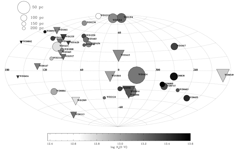
Figure 1: WD locations in Galactic coordinates ($l,b$) for the 39 stars from Table 1 not likely affected by stellar blending (a distance of 100 pc is assumed for the purpose of this plot for WD 0113$+$002). The size of each symbol is inversely proportional to the distance of the line of sight, and the shading of the symbol indicates the total column density of O VI. Note that circles are O VI detections, while the triangles are 2$\sigma$ upper limits for O VI.

The local interstellar medium (LISM) provides an excellent laboratory to probe O VI production processes since the line of sight distances to continuum sources for absorption line spectroscopy are small ($\sim$40 to 200 pc). The LISM is considered to be comprised of the clouds and hot gas within the boundary of the LB which has an asymmetric extension ranging from $\sim$60 to 250 pc. Extensive Na I absorption line studies (Sfeir et al. 1999, Lallement et al. 2003) to map the extent of the LB reveal that the bubble has a sharp boundary determined by a large gradient in the amount of neutral gas. The neutral outer boundary to the local bubble has been traced by Na I (D2) absorption with equivalent widths exceeding 20 mÅ which corresponds to $\log N($H I$)\sim 19.3$. Models for the structure of various clouds situated in the LB are discussed by Linsky et al. (2000) and Redfield & Linsky (2000). In particular Fig. 1 of Linsky et al. (2000) shows the directions where the line of sight to stars in the LB pass through the Local interstellar cloud (LIC), the G cloud, the north Galactic pole cloud, and the south Galactic pole cloud. The distinct cloud identifications suggested by Linsky et al. (2000) are based on the kinematical properties of UV absorption lines seen in the spectra of stars sampling the various cloud directions.

The Copernicus satellite probed O VI absorption toward several relatively nearby stars in the LISM (York 1974; Jenkins 1978a). However, FUSE has completely opened up the range of possible studies. Because of its high radiometric efficiency, measures of O VI absorption toward relatively close-by WDs with FUSE can be achieved in integration times ranging from 10 to 50 ksec. Oegerle et al. (2005) have reported a survey of O VI absorption in the LISM toward 25 white dwarfs ranging in distance from 37 to 224 pc. They reported O VI detections with $\geq 2\sigma$ significance toward 14 of the 25 stars with O VI column densities ranging from somewhat less than $10^{13}$ cm^-2 to $1.7\times 10^{13}$ cm^-2. Oegerle et al. (2005) found an average O VI volume density in the LISM of $2.4\times 10^{-8}$ cm^-3, which is slightly larger than the medium value of $1.7\times 10^{-8}$ cm^-3 measured over kpc distances in the Galactic disk by FUSE (Bowen et al. 2005). Oegerle et al. (2005) attribute the O VI absorption they observe in the LISM to the evaporative interface regions between warm clouds and hot diffuse gas in the Local Bubble (LB). The size and shape of the LB are roughly estimated from the intensity of the diffuse soft X-ray background (Snowden et al. 1998) and the extent of the local region of very weak absorption in the Na I D lines at optical wavelengths (Sfeir et al. 1999, Lallement et al. 2003).

Since the LISM O VI observations discussed by Oegerle et al. (2005) were obtained and analyzed, there have been many additional observations obtained by FUSE of WDs in the LISM. The new observations provide information about O VI absorption along additional lines of sight and provide improved signal-to-noise (S/N) spectra for many of the lines of sight studied by Oegerle et al. In addition, the FUSE data reduction and handling techniques have improved since the version 1.8.7 of the FUSE data reduction pipeline used by Oegerle et al. With these improvements in S/N and data extraction and calibration, it is now possible to not only determine the column densities of O VI toward the WDs but in the higher S/N cases to obtain important information about O VI absorption line velocities and line widths. This allows an evaluation of how the O VI absorption profiles relate to the absorption produced by cooler gas along the line of sight to each white dwarf. Since conductive interface models make specific predictions about the expected O VI line widths and velocity offsets from the cooler gas producing the interface (Böhringer & Hartquist 1987; Slavin 1989; Borkowski, Balbus & Fristrom 1990), it is important to fully quantify the observed character of the O VI absorption in order to test the interface model predictions.

This paper is organized as follows: In §2 we discuss the sample of WDs observed by FUSE and the LISM structures they probe. In §3.1 the FUSE observations and data handling techniques are discussed. In §3.2 and §3.3 problems associated with stellar and circumstellar contamination are discussed. In §3.4 we consider the effects of the WD gravitational redshift. In §3.5 the techniques for determining column densities, line velocities, line widths and their errors are discussed. Comments about absorption along individual lines of sight are found in the Appendix. The observed properties of the LISM O VI absorption are presented in §4. The processes responsible for the presence of O VI in the LISM are considered in §5 with the emphasis being on observational tests of the theory of conductive interfaces. An extension of the results found for the LISM to more distant lines of sight is discussed in §6. The results are summarized in §7. The appendix gives detailed comments about results for selected WDs from the sample.

2 The Sample

We have studied O VI absorption in the FUSE spectra of the 46 WDs listed in Table 1. The sample includes most WD measurements available through the publicly accessible FUSE data archive up to 1 December 2004 but excludes observations where stellar line blending was previously known to severely compromise the interstellar O VI measurement (see §3.2) or where the signal-to-noise level is not adequate for the LISM O VI program. Our sample has considerable overlap with the sample studied by Oegerle et al. (2005), although we use the most recent FUSE extraction and calibration software and when possible have obtained measurements with higher signal-to-noise by incorporating FUSE observations obtained after the 2003 cut off date of the Oegerle et al. data processing.

The various entries in Table 1 include the WD 1950.0 coordinate name and other names, the Galactic latitude, the Galactic longitude, the distance in pc, the estimated effective temperature of the WD, the WD type, the stellar heliocentric velocity, $v_{\star}$, and the heliocentric velocity of low ionization LISM absorption, $v_{\rm LISM}$. The sources for these quantities are given in the footnotes to the table. The distances with listed, errors are from Hipparcos parallax measurements except for WD 1314+293 (HZ 43) where we adopt the distance and error from Van Altena et al. (1995). When no distance error is listed the distance is from photometry and the uncertainty is typically $\pm 20$–30%. The absolute velocities from the literature listed in Table 1 are based on measurements from the IUE satellite (reference 1) or the HST (references 3, 4, and 5) and are more reliable than absolute velocities from FUSE given in parenthesis (this work, reference 2). If no stellar metal lines are detected in the FUSE observations, “NM” for no metals is listed in the column for the stellar heliocentric velocity (see §3.2).

The distribution of the observed WDs on the sky for the 39 stars for which the LISM O VI absorption could be measured or upper limits determined is shown in Fig. 1 where the symbol sizes are inversely proportional to the distance to each object and the symbol grey scale shading denotes the measured column density of O VI  (see §4.1). Seven of the 46 stars are not included in Fig. 1 because stellar contamination of the LISM absorption was judged to be likely (see §3.2). The directions where LISM O VI is detected with $\geq 2\sigma$ significance are displayed as circles with non-detections displayed as triangles. The 39 WDs range in distance from 37 to 230 pc with a median distance of 109 pc.

For several of the brighter WDs in the sample, high resolution spectra ($\lambda/\Delta\lambda\sim 100,000$ and $\sim 40,000$) from the HST obtained with either the Goddard High Resolution Spectrograph (GHRS) or the Space Telescope Imaging Spectrograph (STIS) exist which provide information about the number of discrete LISM absorbing components along the line of sight (see Redfield & Linsky 2002, 2004). Also, in several cases very detailed analysis of the LISM absorption toward selected WDs has been performed with FUSE measurements in order to determine D/H. In some of these cases the analysis has revealed the existence of multiple absorbing components. The component information is important for studying the possible occurrence of O VI in the cloud boundary interface regions. Comments about the WDs with supporting high resolution HST measurements or other observations revealing component structure are given in the Appendix as part of the detailed comments about the O VI absorption toward many of the survey objects.

The picture that emerges from the detailed studies of LISM absorption is that although the lines of sight to the WDs in the LISM extend over relatively small distances, multiple structures are often encountered. For example, along many lines of sight the LISM absorption will be a superposition of absorption in several different structures including the LIC or the G cloud and other more distant clouds. However, in other directions the line of sight structure is very simple.

3 Observations and Measurements

3.1 The FUSE Spectroscopic Data Handling

Descriptions of the FUSE instrument design and inflight performance are found in Moos et al. (2000) and Sahnow et al. (2000). The instrument consists of four channels. Two are optimized for short wavelengths (SiC 1 and SiC 2; 905-1100 Å) and two for longer wavelengths (LiF 1 and LiF 2; 990-1185 Å). The four channels place spectra on two delay line UV detectors and the resulting FUSE data set consists of eight $\sim$90 Å wide spectra identified according to the segments: LiF 1A, LiF 2A, LiF 1B, LiF 2B, SiC 1A, SiC 1B, SiC 2A, SiC 2B. ). The LiF 1A, LiF 2B, SiC 1A, and SiC 2B segment spectra cover the wavelength region of the O VI $\lambda$$\lambda$1031, 1037 doublet. However, we have chosen not to use the SiC 2B data because of the strong fixed pattern noise and relatively low resolution of observations near O VI when using this segment.

Observations in the SiC 1A and LiF 2B segments have $\sim$30% and $\sim$60% of the sensitivity of the LiF 1A segment, respectively. The O VI ISM absorption toward WDs is relatively weak. We have combined the measurements from the three different segments to obtain as high a signal-to-noise (S/N) as possible in the final spectrum even though the spectral resolution is degraded from 20 to approximately 23 ${\rm km\,s}^{-1}$ when combining spectra. In a number of cases early in the FUSE mission, SiC measurements were not obtained because of misalignment of the various channels.

The data set we have processed is listed in Table 2 where we give WD name, the FUSE observation ID, the FUSE aperture, the segments that have been combined into the final co-added spectrum, and the integration times for the segments. The observations were mostly obtained in the LWRS (30″) aperture with a few observations using the MDRS (4″) aperture and 1 line of sight (WD 1634–573) obtained through the HIRS ($1\farcs 25$). Some of the more recent observations obtained with program ID P204 were designed to place the WD at different locations in the LWRS aperture to reduce the effects of detector fixed pattern noise.

The current version of the calibration pipeline software (version 2.0.5 and higher) was employed to extract and calibrate the observations. The details of the processing steps are described by Lehner et al. (2003). The extracted spectra for the separate exposures and segments were aligned in wavelength by a cross-correlation technique and co-added. The cross-correlation provides an excellent alignment because of the presence of strong C II and O I  ISM lines near the weak O VI lines. The combined observations were binned to 4 pixels which corresponds to $\sim$0.025 Å or $\sim$7.5 ${\rm km\,s}^{-1}$. This provides $\sim$3 samples per 20–23 ${\rm km\,s}^{-1}$ resolution element.

When possible, the zero point in the final wavelength scale was established by forcing the ISM lines of C II $\lambda$1036.34 to have the LISM heliocentric velocities found from the more accurate LISM velocities from the literature listed in Table 1 (references 1, 3, 4 or 5). However, when an accurate LISM heliocentric velocity was not available, we simply adopted the heliocentric wavelengths and velocities provided by the standard FUSE pipeline processing of the LiF 1A channel observations. Those velocities are also listed in Table 1 but inside parenthesis. The absolute velocities will therefore be more accurate for those observations incorporating the velocity corrections to the literature. However, since we are primarily interested in the velocity similarities and differences between the O VI absorption and tracers of the neutral gas (O I and C II), this approach is quite acceptable because the velocities of O VI relative to O I and C II are reliable in all cases. Independent studies of O VI absorption toward extragalactic objects by Wakker (private communication) have shown that when using Version 2.05 or later of the data reduction software, the two O VI $\lambda$$\lambda$1031.93, 1037.62 lines are aligned in velocity to better than $\sim$5 ${\rm km\,s}^{-1}$ when using the standard extractions. Since the O VI $\lambda$1037.62 line lies between the ISM O I $\lambda$1039.23 and C II $\lambda$1036.34 lines, it appears that the standard reduction process produces a relative velocity calibration of the O VI, O I, and C II absorption lines that is accurate to $\sim$ 5 ${\rm km\,s}^{-1}$. This is a substantial improvement over the 10 ${\rm km\,s}^{-1}$ velocity error between the two O VI lines present in the earlier version 1.8.7 of the calibration pipeline (see Fig. 2 in Wakker et al. 2003).

Since the path lengths through the LISM are through relatively low density gas, we do not need to worry about possible contamination of the O VI $\lambda$1031.93 measurements from the H₂ (6-0) P(3) and R(4) lines at 1031.19 and 1032.36 Å, respectively. Similarly the O VI $\lambda$1037.62 absorption is not contaminated by the H2 (5-0) R(1) or P(1) lines at 1037.15 and 1038.62 Å, respectively.

3.2 The Effects of WD Gravitational Redshifts

For the WDs listed in Table 1 with detected stellar metal line absorption, it is possible to compare the stellar velocity to the velocity of neutral and weakly ionized gas in the LISM. If the nearby WDs of our sample and the gas of the LISM roughly share a common pattern of motions we would expect the values of the stellar velocity, $v_{\star}$, to exceed that for gas in the LISM by an amount equal to the WD gravitational redshift. Gravitational redshifts of WDs have mostly been studied by observing the radial velocities of WDs and non-degenerate stars in wide binary systems. In a recent study, Silvestri et al. (2001) determined gravitational redshifts for 41 DA WDs by this method and found a distribution of redshifts extending from 8.8 to 58.3 ${\rm km\,s}^{-1}$ for 36 WDs and from 103.6 to 132 ${\rm km\,s}^{-1}$ for 5 WDs. We find the average velocity and velocity dispersion for the lower redshift Silvestri et al. sample are $33.2\pm 11.0$ ${\rm km\,s}^{-1}$. With such a large average gravitational redshift, the effect should be easily seen in a plot of the stellar velocity versus the LISM velocity for a large sample of WDs near to the Sun. In Fig. 2a we compare the values of $v_{\star}$ and $v_{\rm LISM}$ listed in Table 1 and in Fig. 2b display a histogram of number versus $v_{\star}-v_{\rm LISM}$. Although the absolute values of $v_{\star}$ and $v_{\rm LISM}$ are not well determined from our FUSE observations, the relative velocity is accurate to $\sim$ 5 ${\rm km\,s}^{-1}$ when the WD stellar reference lines are the P IV absorptions which are near the LISM C II $\lambda$1036.34 absorption we use to trace neutral and weakly ionized LISM gas. We see from Fig. 2 that $v_{\star}$ exceeds $v_{\rm LISM}$ in all cases except one and the accompanying histogram of number versus $v_{\star}-v_{\rm LISM}$ can be interpreted as an approximate histogram of gravitational redshifts modified somewhat by the different kinematics of gas and stars in the LISM near to the Sun. The average and dispersion of $v_{\star}-v_{\rm LISM}$ we obtain for the 18 stars is $35.2\pm 20.4$ ${\rm km\,s}^{-1}$ which is similar to the average obtained from the Silvestri et al. (2001) sample. It is interesting that the average is similar since the Silvestri et al. (2001) sample is for relatively cool WDs with median temperatures $\sim$10,000 K while our sample is for relatively hot WDs with median temperatures $\sim$40,000 K. A study of this effect could be done more carefully with a larger sample of WDs. However, the measurements are clearly revealing the presence of the WD gravitational redshifts with a simple reference to the rest frame of the LISM. The important result for our investigation of O VI in the LISM is the fact that the WD stellar contamination present in our data set will generally be $\sim$20 to 50 ${\rm km\,s}^{-1}$ redward of the LISM absorption because of the effects of the gravitational redshift.

3.3 Stellar Contamination

Stellar blending of the LISM O VI absorption in the spectra of WDs is a serious problem (Oegerle et al. 2005). The contaminating lines are stellar O VI $\lambda$$\lambda$1031.93 and 1037.62 and in some situations stellar Fe III $\lambda$1032.12 which lies 49 ${\rm km\,s}^{-1}$ redward of the stellar O VI $\lambda$1031.93 line.

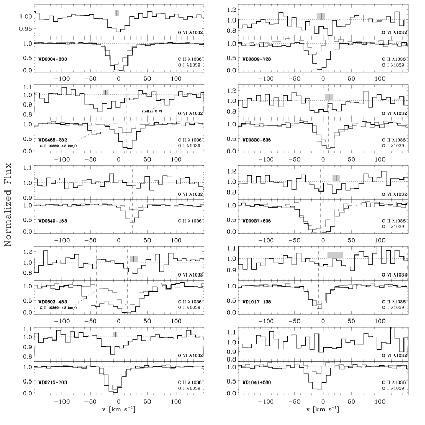
Figure 3: Normalized profiles versus the heliocentric velocity of LISM O VI, C II, and O I absorption. The FUSE velocity was corrected using the LISM values in Table 1, except for the cases where we do not have accurate absolute velocities. The vertical dotted line is the C II  average velocity. The tick mark above the O VI profile is the O VI AOD velocity with the gray area showing its error. We only display the 2$\sigma$ upper limits from Table 1 when $\log N($O VI$)<13.00$.

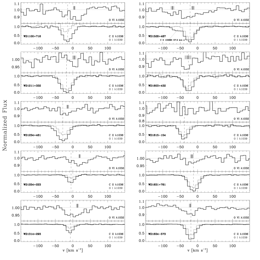
Figure 3: continued.

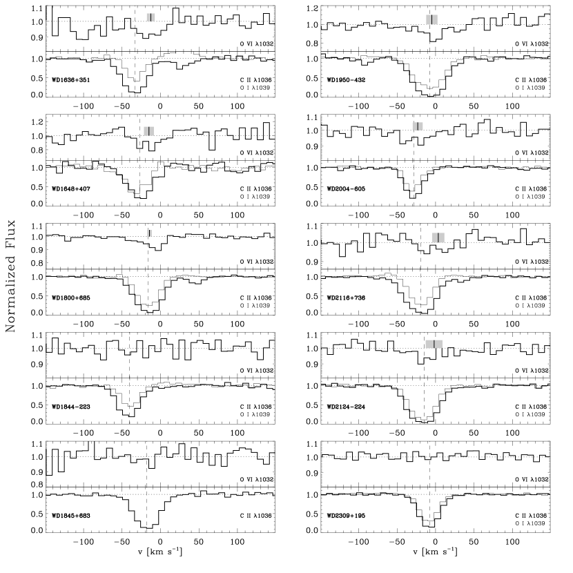
Figure 3: continued.

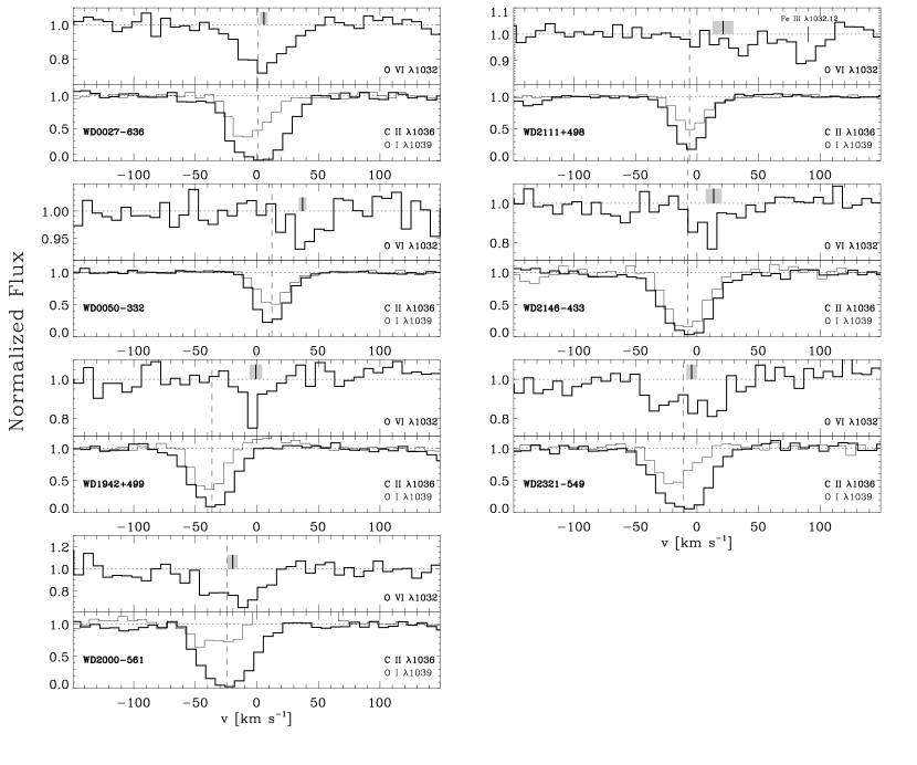
Figure 6: Normalized profiles for O VI, C II, and O I versus the heliocentric velocity. Same as in Fig 3 except for those WDs where much of the observed O VI absorption may be stellar rather LISM (see § 3.2).

For WDs with $T_{\rm eff}<40,000$ K, the NLTE model atmosphere calculations of Oegerle et al. (2005; see their Fig. 5) suggest that the stellar O VI absorption should be very weak provided the oxygen abundance is less than $\log({\rm O/H})=-5.0$. Above 40,000 K, the stellar O VI will be weak or strong depending on the abundance of oxygen in the photosphere. Contamination from Fe III  near O VI can occur in the cooler WDs. When stellar O VI or Fe III is present, stellar lines of other elements and ions will also generally be observable in the wavelength region covered by the FUSE spectra. The Oegerle et al. model atmosphere calculations for particular WDs with stellar comtamination in the lines of O VI and Fe III shown in their Fig. 6 illustrate some of the absorption features accompanying stellar O VI and/ or stellar Fe III. In the higher temperature WDs stellar O VI is accompanied by stellar P IV $\lambda$$\lambda$1030.51, 1033.11. In the four hot WD cases shown by Oegerle et al., the P IV $\lambda$1031.51 line has a strength relative to O VI $\lambda$1031.93 ranging from $\sim 3\times$ stronger to $\sim 2\times$ weaker although there are WDs with extremely strong stellar O VI with no detectable P IV (see Fig. 3 for WD 2156–545 in Oegerle et al. 2005 and Fig. 2 for WD 0131–163 in Lehner et al. 2003). However, WD 0131–163 also shows strong stellar Si IV $\lambda$1066.63 and P V $\lambda$1117.98. This suggests that a first evaluation of the possibility of stellar O VI contamination can be based on the presence or absence of absorption by P IV $\lambda$$\lambda$1030.51, 1033.11, P V $\lambda$1117.98, and Si IV $\lambda$1066.63. For Si IV $\lambda$1066.63, allowance must be made for ISM contamination from Ar I $\lambda$1066.66 which can be evaluated with reference to the blend free ISM Ar I $\lambda$1048.22 absorption. The possible stellar contamination from Fe III $\lambda$1032.12 can be evaluated with reference to other stellar Fe III lines including Fe III $\lambda$$\lambda$1030.92, 1033.30.

For all the stars in our program listed in Table 1 we produced velocity plots showing a combination of potential stellar and potential ISM absorption lines including P IV $\lambda$$\lambda$1030.51, 1033.11, P V $\lambda$1117.98, Fe III $\lambda$$\lambda$1030.92, 1032.12, 1033.30, Si IV $\lambda$1066.63, Ar I $\lambda$$\lambda$1048.22, 1066.66, Fe II $\lambda$1144.94, and O VI $\lambda$1031.93. The ISM Fe II $\lambda$1144.94 observation allows us to calibrate the velocity of the P V $\lambda$1117.98 stellar absorption with the detector segments containing the O VI absorption. An evaluation of the velocity plots for the presence of stellar absorption lines allowed us to identify the possibility of stellar contamination of the LISM O VI $\lambda$1031.93 absorption and the velocity of the contamination. Additional information about possible stellar line blending can be inferred from the WD studies of Holberg et al. (1998) and Bannister et al. (2003) of spectra in the wavelength range from $\sim$1150 to $\sim$1850 Å obtained by the IUE satellite and/or the spectrographs flown on the HST including the GHRS and STIS.

In Table 1 we list values of the WD stellar velocity, $v_{\star}$, when known either from the literature (Table 1 reference 1, 3, 4, and 5) or from the FUSE observations of one or more of the stellar lines of P IV, P V  Si IV, and Fe III listed above (Table 1 reference 2). Velocities based on the FUSE observations alone are given in parenthesis since the absolute velocity is not well determined but the relative velocities are accurate. In a large number of cases denoted with “NM” in Table 1, no stellar metal lines have been seen with FUSE or IUE or HST.

Based on our evaluation of the stellar/interstellar absorption line velocity plots and other sources of information about stellar contamination we have rejected from our LISM study the following 7 WDs from Table 1 because of likely or possible contamination of the LISM O VI $\lambda$1031.92 absorption by stellar O VI absorption. We give the reasons for the rejection in the following brief discussions of each object.

WD 0027–636 ($T_{\rm eff}=63,724$ K). The P IV and Fe III lines are not detected. However, the Si IV and P V absorption is very strong and occurs near 30.2 ${\rm km\,s}^{-1}$ which is close to the velocity of the observed O VI absorption at $23.2\pm 4.4$ ${\rm km\,s}^{-1}$. A substantial amount of stellar O VI contamination is likely given the high stellar temperature.

WD 0050–332 (GD 659) ($T_{\rm eff}=36,000$ K). We detect strong P V but do not detect P IV or Si IV. Bannister et al. (2003) note that GD 659 has photospheric absorption at $34.3\pm 0.17$ ${\rm km\,s}^{-1}$  and possibly weaker circumstellar absorption at $-2.97\pm 3.00$ ${\rm km\,s}^{-1}$. The photospheric absorption is seen in Si IV, C IV and N V in STIS and IUE spectra and in P V in the FUSE observations. This photospheric absorption is well aligned with the O VI we detect at $39.8\pm 3.1$ ${\rm km\,s}^{-1}$ and we conclude stellar O VI contamination is possible even though $T_{\rm eff}<40,000$ K. This is a conservative conclusion since O V $\lambda$1371.30 is evidently not seen in the IUE spectrum discussed by Holberg et al. (1998).

WD 1942+499 ($T_{\rm eff}=34,400$ K). Strong Si IV $\lambda$1066.63 absorption is detected near $-5$ ${\rm km\,s}^{-1}$ which is close to the O VI absorption velocity of $-0.8\pm 5.1$ ${\rm km\,s}^{-1}$. Stellar O VI contamination is possible even though $T_{\rm eff}<40,000$ K.

WD 2111+498 ($T_{\rm eff}=37,360$ K). Very strong stellar P IV, Si IV, and Fe III are found at 28.9 ${\rm km\,s}^{-1}$ which is near the velocity of the observed O VI absorption at $21.1\pm 8.4$ ${\rm km\,s}^{-1}$. The Fe III $\lambda$1032.12 feature near the stellar or interstellar O VI  is also evident in the spectrum. Since the P IV and Si IV absorption is so strong, the $W_{\lambda}=9.5\pm 3.1$ mÅ  O VI $\lambda$1031.93 feature detected is probably contaminated by stellar O VI even though $T_{\rm eff}<40,000$ K. This is a conservative conclusion since O V $\lambda$1371.30 is evidently not seen in the IUE spectrum studied by Holberg et al. (1998).

WD 2000–561 ($T_{\rm eff}=47,299$ K). Very strong stellar P IV and Si IV are found at $-15.4$ ${\rm km\,s}^{-1}$  which is close to the $-19.6\pm 4.1$ ${\rm km\,s}^{-1}$ velocity of the observed O VI absorption. Given the large value of $T_{\rm eff}$, stellar O VI contamination is likely.

WD 2146–433 ($T_{\rm eff}=67,912K$). Very strong stellar P IV and Si IV are found at 27.0 ${\rm km\,s}^{-1}$ which is near $13.5\pm 6.4$ ${\rm km\,s}^{-1}$, the observed O VI velocity. Given the high value of $T_{\rm eff}$, stellar O VI contamination appears likely.

WD 2321–549 ($T_{\rm eff}=45,860$ K). Very strong stellar P IV and Si IV are found at 9.9 ${\rm km\,s}^{-1}$. Approximately 50% of the observed O VI absorption occurs near this velocity and is likely stellar in origin because of the large value of $T_{\rm eff}$. Rather than trying to separate the stellar and interstellar O VI absorption, the object was rejected from inclusion in the final LISM sample.

We also rejected from consideration and inclusion in Table 1 the other WDs that Oergele et al. (2005) have previously shown to be contaminated. These include WD 0501+527, WD 2156–546, WD 2211–495, and WD 2331–475.

In several cases, we identify strong stellar features in the FUSE WD spectrum but have retained the star for our LISM O VI study. The 4 stars include:

WD 0455–282 ($T_{\rm eff}=57,200$ K). Strong stellar P IV, Si IV, C IV and N V absorption is seen at 69.6 ${\rm km\,s}^{-1}$ which is well displaced from the LISM O VI, C II, and O I absorption. O V $\lambda$1371.30 is evidently not seen in the IUE spectrum studied by Holberg et al. (1998) although stellar O VI near 80 ${\rm km\,s}^{-1}$ is evident in the FUSE spectrum shown in Fig. 3.

WD 0603–483 ($T_{\rm eff}=35,322$ K). Stellar P V is detected near 41 ${\rm km\,s}^{-1}$ but is not aligned with the O VI absorption at $25.6\pm 7.1$ ${\rm km\,s}^{-1}$.

WD 1634–573 (HD 149499B) ($T_{\rm eff}=49,500$ K). We detect what could be P IV $\lambda$1033.11 near $-15$ ${\rm km\,s}^{-1}$ but do not see the corresponding P IV $\lambda$1030.51 absorption. Holberg et al. (1998) report stellar Si IV and C IV at $v_{\star}=0.61\pm 2.15$ ${\rm km\,s}^{-1}$ and LISM absorption at $v_{\rm LISM}=-19.6$ ${\rm km\,s}^{-1}$. The O VI absorption we see toward this star is well aligned with the LISM absorption of C II and O I. Although some stellar O VI contamination may be present, it does not appear to be affecting our measurement.

WD 1950–432 ($T_{\rm eff}=41,339$ K). Stellar P V is detected at 40 ${\rm km\,s}^{-1}$ but it is not aligned in velocity with the O VI absorption at $-4.9\pm 7.3$ ${\rm km\,s}^{-1}$.

There are a number of stars that potentially have stellar contamination of O VI as judged from the stellar/ISM velocity plots but for which no O VI (stellar or interstellar) has been detected. Since these objects provide good upper limits to the interstellar value of $\log N($O VI), they have been retained for our LISM study. WDs in this category include:

WD 0416+402 ($T_{\rm eff}=35,227$ K). Strong stellar Fe III $\lambda$1030.92 and Si IV $\lambda$1066.63 are found near 79 ${\rm km\,s}^{-1}$. However, stellar or ISM O VI is not detected.

WD 0802+413 ($T_{\rm eff}=45,394$ K). Photospheric P V $\lambda$1117.98 is strong at 59 ${\rm km\,s}^{-1}$. However, stellar or ISM O VI is not detected.

We believe it is unlikely that the 39 WDs retained for our LISM study are seriously affected by stellar O VI blending. However, it would take a very extensive stellar spectroscopic investigation, well beyond the scope of our ISM study, to actually prove in all cases that stellar blending can be ignored.

3.4 Circumstellar Contamination

Non-photospheric circumstellar absorption has been found in the spectra of 5 of 44 DA WDs observed by Holberg et al. (1998). An additional four examples have been identified by Bannister et al. (2003) among a group of 23 WDs. The features have shown up as highly ionized ions (Si IV, C IVand N V) seen in IUE spectra (Holberg et al. 1998) and/or STIS spectra (Bannister et al. 2003). A number of origins for these features include photoionization of the local interstellar environment of the WD (Dupree & Raymond 1983), matter in the WD gravitational potential well, mass loss in a WD wind, matter in a surrounding ancient planetary nebula, and matter from a companion star. One object on our list, WD 0050–332 (GD 659) with possible circumstellar contamination, has already been discussed §3.2 and has been rejected from our LISM study because of the possibility of strong stellar contamination.

WD 0455–282 with $T_{\rm eff}=57,200$ K is another star in our sample possibly having circumstellar contamination problems. Holberg et al. (1998) note that Si IV and C IV absorption is seen in IUE spectra at $v=16.21\pm 2.66$ ${\rm km\,s}^{-1}$  while the photospheric velocity is $69.60\pm 1.97$ ${\rm km\,s}^{-1}$. Photospheric O VI is detected in this WD but at a velocity well removed from the LISM absorption. While circumstellar contamination is potentially a problem, our observations show the O VI absorption near 16 ${\rm km\,s}^{-1}$ provides only a small ($\sim$10–15 %) contribution to the total O VI absorption.

We are not aware that any of the other stars in our sample have been identified as possibly having circumstellar contamination problems. While the frequency of occurrence of circumstellar contamination appears to be relatively low, we need to be aware that circumstellar contamination may adversely affect some of the WDs in our LISM study.

3.5 Measurements of O VI Column Densities, Velocities, and Line Widths

Continuum normalized absorption line profiles for the lines of O VI $\lambda$1031.93, C II $\lambda$1036.34, and O I $\lambda$1039.23 displayed on a heliocentric velocity scale are shown in Fig. 3 for the 24 WDs for which the LISM O VI $\lambda$1031.93 line has been detected with $\geq 2\sigma$ significance along with profiles for 4 WDs where no O VI has been detected. Absorption lines produced by contaminating stellar features are identified on several of the panels. In Fig. 4 we display the line profile plots for the 7 WDs for which we believe the LISM O VI absorption is likely contaminated by stellar O VI as discussed in §3.2.

O VI absorption line measurements are listed in Table 3 for all the objects listed in Table 1. The O VI $\lambda$1031.93 absorption line equivalent width, $W_{\lambda}$, is listed in column 9 with the heliocentric velocity range of the integration listed in column 11. When we believe stellar contamination is likely affecting the measurements as discussed in §3.2, the equivalent width of the O VI $\lambda$1031.93 line is given in parenthesis.

The continuum placement procedure for measuring the absorption utilized Legendre polynomials and the algorithm described by Sembach & Savage (1992) which provides an estimate of the continuum uncertainty. The listed $\pm 1\sigma$ errors for the equivalent widths in Table 3 are from a quadrature addition of the statistical error and the continuum placement error. The fixed pattern noise errors for these combined observations from multiple segments are estimated to be $\sim$2–3 mÅ. When an equivalent width and error is listed in Table 3, the detection significance is $\geq 2\sigma$. When LISM O VI is not detected with a significance of 2$\sigma$ or greater we list the 2$\sigma$ upper limit to the value of $W_{\lambda}$. The actual significance of the detection, $W_{\lambda}/\sigma$, is given in column 10.

Two methods have been used to measure the O VI absorption velocities, line widths, and column densities listed in Table 3. For method 1, the entries for $\bar{v}_{f}$, $b_{f}$, $\log N_{f}$, in columns 2, 3, and 4 are based on Voigt profile fits of single absorption components with velocity, $\bar{v}_{f}$, Doppler parameter, $b_{f}$, and logarithmic O VI column density, $\log N_{f}$. The fit results and the errors were obtained using the Voigt component fitting software of Fitzpatrick & Spitzer (1997). The fit results listed are based on a simultaneous fit to both members of the O VI $\lambda$$\lambda$1031.93, 1037.62 doublet even though the $\lambda$1037.62 line is only clearly detected with $\geq 2\sigma$ significance in 8 of the 30 WDs (see Table 4). The FUSE instrumental function was assumed to be a Gaussian with FWHM $=20$ ${\rm km\,s}^{-1}$. The errors on $b_{f}$ are large for the lower significance detections of the $\lambda$1031.93 line with $2\sigma<W_{\lambda}<4\sigma$. In those cases the values of $b_{f}$ are not listed in Table 3. Two examples of the simultaneous component fit process are shown in Fig. 5. These examples are for the well-observed stars WD 1254+223 and WD 1314+293.

For method 2, the entries for $\bar{v}_{a}$, $b_{a}$, $\log N_{a}$, in columns 5, 6, and 7 in Table 3 are based on the apparent optical depth (AOD) method of Savage & Sembach (1991) applied to the $\lambda$1031.93 absorption line. The O VI absorption profiles were converted into apparent column densities per unit velocity $N_{a}(v)=3.768\times 10^{14}\ln[F_{c}/F_{\rm obs}(v)]/(f\lambda)$, where $F_{c}$ is the continuum flux, $F_{\rm obs}(v)$ is the observed flux as a function of velocity, $f$ is the oscillator strength of the absorption and $\lambda$ is in Å. The values of $\bar{v}_{a}$, $b_{a}$, $\log N_{a}$, listed in columns 5, 6, and 7 are obtained from $\bar{v}_{a}=\int vN_{a}(v)dv/N_{a}$, $b_{a}=[2\int(v-\bar{v}_{a})^{2}N_{a}(v)dv/N_{a}]^{1/2}$, and $N_{a}=\int N_{a}(v)dv$.

Again for the lower significance detections with $2\sigma<W_{\lambda}<4\sigma$, the errors on $b_{a}$ are so large the values of $b_{a}$ are not listed. In those cases where O VI $\lambda$1031.93 absorption was not detected with a significance $\geq 2\sigma$, we report the 2$\sigma$ upper limit to the column density in the column labeled $\log N_{a}$ in Table 3 by assuming the line is on the linear part of the curve of growth. This is a valid assumption given the breadth and weakness of the O VI absorption. The $f$-values for the O VI $\lambda$$\lambda$1031.93, 1037.62 lines of 0.133 and 0.0658 used in our derivations of the O VI column density are taken from Morton (2003).

For the 8 WDs for which the O VI $\lambda$1037.62 line was also detected with a significance $\geq 2\sigma$ the equivalent widths and ADO values of $\bar{v}_{a}$, $b_{a}$, $\log N_{a}$ are listed in Table 4. When both O VI absorption lines are detected the best estimates of the O VI absorption properties are from the simultaneous Voigt profile fits listed in Table 3 or from an average of the two reported values of $N_{a}$.

The O VI absorption lines are broad, relatively weak and are unlikely to contain unresolved saturated structures. Since O VI peaks in abundance at $T=2.8\times 10^{5}$ K, the thermal Doppler width of a single component containing O VI is expected to be $b=17.1$ ${\rm km\,s}^{-1}$ corresponding to FWHM $=28.5$ ${\rm km\,s}^{-1}$. With a resolution of 20–23 ${\rm km\,s}^{-1}$, FUSE is expected to nearly fully resolve the O VI absorption implying the observed absorption profiles are probably a good representation of the true O VI absorption. In the 8 cases where both components of the O VI doublet have been detected (see Table 3 and 4) a comparison of the two values of $\log N_{a}$ based on the weak and strong line of the doublet reveals good agreement. This confirms that line saturation problems are not a difficulty when deriving values of $\log N($O VI). If saturation were a problem we would expect the value of $N_{a}$ from the strong line to be smaller than the value from the weak line.

In Fig. 6 we compare the results from the two methods we have used to derive the O VI absorption parameters for the WDs not affected by stellar contamination. In Fig. 6a the AOD and profile fit column densities are compared. The solid line shows the 1:1 relationship. The correspondence is very good. However, we prefer the AOD results since they are not dependent on assumptions about the line shape or component structure. In Fig. 6b we compare the AOD results from Table 3 with the earlier measures of $\log N($O VI) based on the equivalent widths measured by Oegerle et al. (2005). The agreement is good, although in a number of cases our measurements have a higher statistical significance since for some of the WDs our results are based on combining more recent measurements with the older observations studied by Oegerle et al. Therefore, we were able to convert several of the earlier upper limits into detections. In Fig. 6c we compare the AOD and profile fit values of the average O VI velocity. The correspondence between the two ways of measuring $\bar{v}($O VI) is good. In Fig. 6d we compare the AOD and profile fit results for $b($O VI) for the more reliable cases, where the O VI detection significance for the strong line of the doublet exceeds 4$\sigma$. The two methods yield similar results although the AOD method does not require assumptions about line shape or component structure. We conclude that both the profile fit method and the AOD method yield good measures of $\log N($O VI) and $\bar{v}($O VI). The two methods provide reliable estimates of $b($O VI) provided $W_{\lambda}\geq 4\sigma$.

An important aspect of our investigation involves studying the kinematical relationships between the absorption by LISM O VI and other tracers of gas in the LISM. We therefore compare the absorption velocities of O VI with those of O I and C II in Table 5 for the 24 WDs listed in Table 3 not affected by stellar contamination and with $W_{\lambda}\geq 2\sigma$. For all three ions we list the average absorption velocity for the ion determined from the AOD method. Table 5 therefore lists for each WD with detected O VI absorption, $\bar{v}_{a}($O VI), $\bar{v}_{a}($C II), $\bar{v}_{a}($O I), and $\bar{v}_{a}($O VI$)-\bar{v}_{a}($C II). Table 1 identifies those cases where the absolute velocities are referenced to the more reliable IUE or HST measurements (Table 1 references 1, 3, 4, and 5). However, velocity differences among O VI, O I, and C II within the FUSE observations listed in Table 5 are reliable in most cases since the relative velocity calibration error is $\sim 5$ ${\rm km\,s}^{-1}$.

4 Properties of O VI Absorption

4.1 O VI Column Densities

Results are reported for O VI LISM absorption unaffected by stellar contamination toward 39 WDs in Table 3. The O VI $\lambda$1031.93 line is detected with $\geq 2\sigma$ significance toward 24 of the 39 WDs. If we increase the required significance of a detection to $\geq 3\sigma$, these numbers change to 17 of 39 WDs. In 12 cases where the detection significance $\geq 4\sigma$ it is possible to obtain high quality information about the line width and shape. For 8 of these higher significance detections there is also reliable information provided by the O VI $\lambda$1037.62 absorption line. The O VI column densities for the 24 $\geq 2\sigma$ detections range from $\log N_{a}($O VI$)=12.38$ (WD 1211+332) to 13.60 (WD 0809–728) with a median of 13.10. In the following discussions we will make use of the AOD value of $\log N($O VI) for the stronger $\lambda$1031.93 absorption since no assumptions are required about profile shape or component structure when determining a column density via the AOD method.

The distribution of O VI absorption on the sky is illustrated with the symbols and grey scale coding of Fig. 1. The irregular distribution of O VI on the sky is well illustrated in the figure. The most striking column density contrast is in the direction of the north Galactic pole with $b>80\arcdeg$ where there are two WDs including WD 1254+223 and WD 1314+293 with similar distances (67 pc) and similar column densities ($\log N($O VI$)=13.10$ and 12.94). The results for these two stars are in stark contrast to the result for the third north Galactic polar WD 1211+332 with $d=115$ pc and $\log N($O VI$)=12.38$. The range in average line of sight O VI volume density among these three stars is a factor of six.

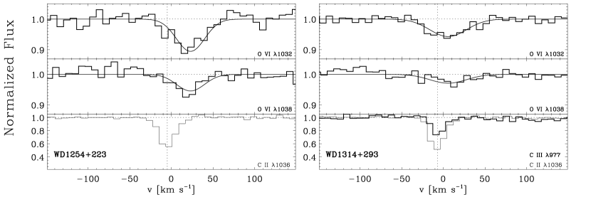
Figure 7: Normalized flux versus heliocentric velocity and one component fit to the O VI absorption lines toward WD 1254+223 and WD 1314+293. C II absorption is displayed for both stars. For WD 1314+293 C III is also displayed.

In Fig. 7 $\log N_{a}($O VI) is plotted against $\log d$ (pc) with the distance to each WD taken from Table 1. The filled circles are the $\geq 2\sigma$ detections and the open circles with the attached arrow are the 2$\sigma$ upper limits. The open diamonds (without or with limit arrows) show the values of $\log N($O VI) or the $\sim$2$\sigma$ limits from the Copernicus Satellite survey of O VI  (Jenkins 1978a) toward hot stars with $d<1000$ pc. There is a general trend of increasing $N_{a}($O VI) with distance, although the dispersion in the measurements indicates a considerable amount of irregularity in the O VI absorption in the LISM and beyond. The solid line in Fig. 7 shows the relation between $\log N_{a}($O VI) and $\log d$ corresponding to the average value of $n_{a}($O VI$)=3.6\times 10^{-8}$ cm^-3 we obtain for the FUSE WD sample (see below). The dashed line shows the median value, $1.7\times 10^{-8}$ cm^-3, obtained when the FUSE measurements of O VI in the Galactic disk toward 150 stars with distances up to $\sim$8 kpc (Bowen et al. 2005) are combined with the Copernicus measurements of Jenkins (1978a) of stars with distances up to $\sim$2 kpc.

4.2 O VI Average Density

Although the actual volume density distribution of O VI in the ISM is unknown, it is useful to examine the behavior of the O VI volume density, $n_{a}($O VI$)=N_{a}($O VI$)/d$, averaged along each WD line of sight. The volume density along different lines of sight and its dispersion can be studied as a function of position in the Galaxy and the values can be compared to theoretical expectations for different O VI production processes.

The value for $n_{a}($O VI) or the density limit for each WD is listed in column 8 of Table 3 for 39 WDs. The limit to $n_{a}($O VI) for WD 0113+002 assumes a WD distance of 100 pc. The values of $n($O VI) for the 24 $\geq 2\sigma$ detections range from $(0.68-13.0)\times 10^{-8}$ cm^-3. The distribution on the sky of the average line of sight physical density is displayed in Fig. 8 with the same symbol coding that was used in Fig. 1. There is considerable irregularity to the distribution of the values of $n_{a}($O VI) on the sky although the highest average density line of sight cluster in the general direction toward $l\sim 270\arcdeg$ and $b\sim-15\arcdeg$.

Medians, averages, and dispersions for $n_{a}($O VI) derived from several subsets of the 39 WD sample are listed in Table 6. The first entries in Table 6 are the values for the 39 stars treating the 15 2$\sigma$ upper limits as detections. The second entries are the values for the 24 stars where O VI is detected with $\geq 2\sigma$ significance.

Since 15 of 39 measurements are upper limits to $n_{a}($O VI), we need to seek a better method to determine the average value of $n_{a}($O VI) from our data sample. Feigelson & Nelson (1985) and Isobe et al. (1986) discuss the Kaplan-Meier product-limit estimator method, which is a nonparametric univariate survival analysis technique that can be used to estimate the mean of a set of data points containing upper limits. The technique can be applied to variables with any underlying distribution so long as the observations are a random sampling of the distribution and the detections and limits are part of the same distribution. The Kaplan-Meier analysis technique applied to the 24 detections and 15 2$\sigma$ upper limits yields $n_{a}($O VI$)=(3.6\pm 0.5)\times 10^{-8}$ cm^-3, where the error is the Kaplan-Meier error on the average value rather than the dispersion about the average.

The average density we estimate for O VI is considerably larger than the value $2.4\times 10^{-8}$cm^-3 found by Oegerle et al. (2005) along the sight line to 25 LISM WDs. O VI was detected with greater than 2$\sigma$ significance toward 13 of the 25 stars in the Oegerle et al. sample. The derived value of $n($O VI) is sensitive to how the detections and limits are included in the averaging process. Oegerle et al. averaged all the data values for the 25 WDs in their sample treating non-detections as detections and even treating negative non-detections as negative densities in the averaging. Many of the non-detections have values of $n($O VI) close to zero which introduces a large downward bias in the estimate of the average value of $n($O VI). The Kaplan-Meier analysis technique we have adopted for dealing with the upper limits is a much better approach for estimating the average value of O VI. To test if there is a fundamental difference between the Oergerle et al. measurements and our measurements, we converted the Oegerle et al. column densities into a set of 13 detections and 12 2$\sigma$ upper limits. After adopting our distances from Table 1, we determined O VI volume densities and 2$\sigma$ upper limits. We then used the Kaplan-Meier analysis technique to estimate the average volume density from the Oegerle et al. sample and found $n($O VI$)=(3.1\pm 0.4)\times 10^{-8}$ cm^-3 which is very similar to the average density we have obtained from our measurements. The estimate of the average value of the LISM O VI volume density from the Oegerle et al. data set agrees with our value when the upper limits are properly included in the averaging process.

If we restrict our estimate of the average value of $n($O VI) to the 17 WDs with $d<100$ pc (including 9 $\geq 2\sigma$ detections and 8 upper limits) we obtain a sample dominated by WDs within the LB. If we again use the Kaplan-Meier analysis technique to evaluate the effects of the upper limits on the average, we obtain $n($O VI$)=(4.0\pm 0.8)\times 10^{-8}$ cm^-3 which is similar to the value of $3.6\pm 0.5$ cm^-3 obtained for the entire sample of 39 WDs.

The average value of $n($O VI$)=3.6\times 10^{-8}$ cm^-3 we obtain for O VI in the LISM toward 39 WDs is 2.1 times larger than the median value $n($O VI$)=1.7\times 10^{-8}$ cm^-3 obtained for the much more distant sample of hot stars surveyed by FUSE by Bowen et al. (2005). There is a modest excess of O VI in the LISM compared to the more distant interstellar regions.

4.3 $N($O VI) vs $N($O I) in the LISM

It is of interest to compare the observed column density of O VI to that for other tracers of LISM gas along the line of sight to each WD. Currently, the largest body of measurements for other important species toward our WD sample exists for O I from Lehner et al. (2003). In Table 7 we list the WD, distance from Table 1, $\log N_{a}($O VI) from Table 3, and values of $\log N($O I) which are mostly from Lehner et al. (2003). O I is an important tracer of gas in the LISM because the measured value of $\log N($O I), is useful in determining if the line of sight passes through the dense boundary wall of the LB. For O/H $=(3.45\pm 0.19)\times 10^{-4}$ which is the value measured in the LISM (Oliveira et al. 2005), $\log N($O I$)=15.8$ implies $\log N($H I$)\sim 19.3$ corresponding to the bubble wall definition of Sfeir et al. (1999). Those lines of sight where $\log N($O I$)<15.6$ probably do not extend through the boundary of the LB wall. For $\log N($O I$)>15.8$ the LB wall is probably penetrated. For the intermediate cases with $15.6<\log N($O I$)<15.8$, the line of sight may or may not pass through the LB wall. If the wall does occur in this column density range, one might expect to observe a change in the behavior of O VI if the O VI  absorption occurs in or near the boundary of the LB.

Fig. 9 shows $\log N($O VI) versus $\log N($O I) for the 18 WDs for which both O VI and O I column density measurements exist (ignoring WD 0455–282). There are only 4 WDs with $\log N($O I$)<15.6$. O VI is detected toward 3 of these 4 WDs and the median value of $\log N_{a}($O VI) is 12.94. The 14 WDs with $\log N($O I$)>15.6$ show a large spread in $\log N($O VI) with a median value of 12.95. Three of the WDs that should lie near or beyond the bubble wall show the smallest values of $\log N($O VI) in the sample. These include WD 1211+332 with $\log N($O VI$)=12.38\pm\,^{0.17}_{0.28}$, WD 1631+781 with $\log N($O VI$)=12.52\pm\,^{0.12}_{0.17}$, and WD 2309+105 with $\log N($O VI$)<12.53$. There are 3 WDs out of a total of 8 beyond the bubble wall displaying an excess of O VI compared to the closer WDs. These are WD 0715–703 with $\log N($O VI$)=13.23\pm 0.07$, WD 1017–138 with $\log N($O VI$)=13.29\pm 0.11$, and WD 1528+487 with $\log N($O VI$)=13.27\pm 0.06$. The 0.2 to 0.3 dex excess in $\log N($O VI) toward these 3 objects could be due to the bubble wall. The excess corresponds to a bubble wall contribution to $\log N($O VI) of $\sim$ 13.0. Note that the objects beyond the bubble wall with high and with low values of $\log N($O VI) are widely distributed on the sky. The presence of O VI in the LB wall is suggested by the excess O VI recorded along 3 of the 8 lines of sight through the wall. The absence of a strong LB wall signature in O VI for the 5 lines of sight could be due to the magnetic suppression of conduction in the warm-hot gas interface or to the absence of hot gas at the LB wall.

4.4 O VI Line Widths

When LISM O VI is detected with $\geq 4\sigma$ significance, it is possible to obtain reliable measures of the line width, $b$ (${\rm km\,s}^{-1}$), either from the AOD or profile fit methods (see Fig. 6d). The AOD values of $b$ are slightly larger than the profile fit values, probably partly due to the fact that the profile fit values of $b$ allow for the instrumental blurring while the AOD values of $b$ are simply based on a direct integration of the observed profile. The observed profile fit line widths for the 11 WDs with $W_{\lambda}/\sigma>4$ tracing LISM gas range from $15.0\pm 3.5$ ${\rm km\,s}^{-1}$ for WD 1800+685 to $36.2\pm 7.3$ ${\rm km\,s}^{-1}$ for WD 1528+487. The median and the average and dispersion of $b_{f}$ are 20.5 ${\rm km\,s}^{-1}$ and $23.0\pm 5.6$ ${\rm km\,s}^{-1}$  respectively. In CIE O VI peaks in abundance at $2.8\times 10^{5}$ K (Sutherland & Dopita 1993). At this temperature the thermal Doppler line width of O VI is $b=17.1$ ${\rm km\,s}^{-1}$ which is close to the minimum value of $b_{f}$ observed. A line with $b_{f}$ as large as 36.2 ${\rm km\,s}^{-1}$ implies $T=1.3\times 10^{6}$ K if the broadening is dominated by thermal Doppler broadening. Very little O VI exists at temperatures this large under conditions of CIE (Sutherland & Dopita 1993). Therefore, the broader O VI profiles could be tracing multiple component O VI absorption or the kinematic flow of the O VI in a single absorbing structure.

In several of the highest S/N cases the observed line profiles are strongly suggestive of the blending of multiple absorption components. Examples include WD 0455–282 and WD 1528+487 (see Fig. 3). However, the S/N in most of the observations is not adequate to warrant fitting multiple absorption components to the observed line profiles of the weak O VI absorption.

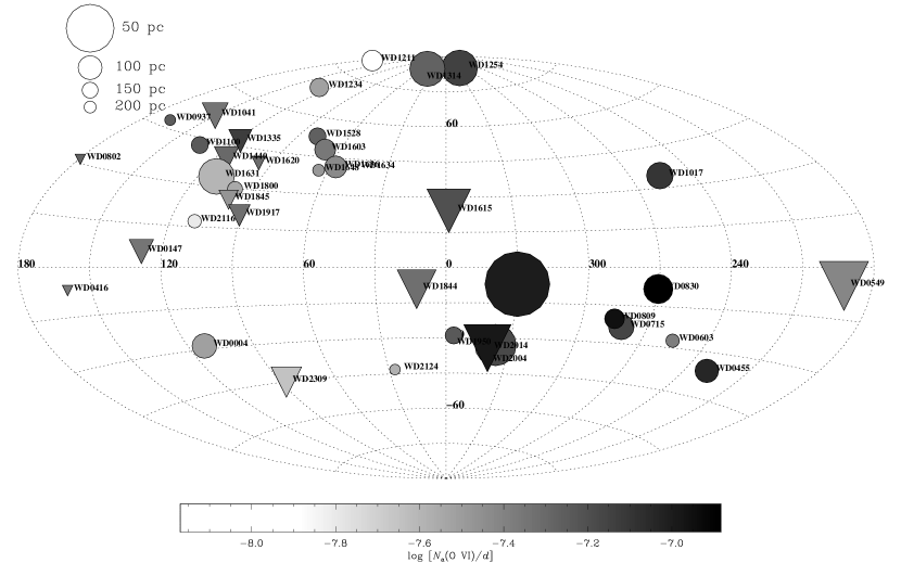
Figure 10: WD locations in Galactic coordinates ($l,b$) for the 39 stars from Table 1 not likely affected by stellar blending problems. Same symbol code as Fig. 1 except the grey scale indicates the average line of sight density $N_{a}($O VI$)/d$ (circles) or density limit (triangles).

The O VI column density and Doppler parameter for LISM lines of sight are correlated. In Fig. 10a $\log N_{a}($O VI) is plotted against $b_{a}$ for the 11 $\geq 4\sigma$ LISM detections listed in Table 3. The histogram of the values of $b_{a}$ for the 11 $\geq 4\sigma$ LISM detections is shown in Fig. 10b. The correlation of $\log N_{a}($O VI) and $b_{a}$ has previously been shown to extend from the LISM to the Galactic disk and halo and beyond (Heckman et al. 2002; Savage et al. 2003). The trend observed in the LISM could be the result of the superposition of contributions to $\log N_{a}($O VI) and $b_{a}$ from multiple interfaces displaced in velocity. This explanation is supported by the fact that those lines of sight with very broad O VI profiles also have very strong and broad multicomponent C II absorption. Examples include WD 0455–282, WD 0830–535, and WD  1528+487 (see Fig. 3). However, several lines of sight with particularly simple and narrow C II absorption profiles including WD 1254+223 and WD 1314+293 exhibit O VI absorption that may be affected by the outflow from an evaporative interface (see §5.1.2). The O VI profile breadths for gas in the LISM evidently are influenced by a combination of several effects in addition to the thermal Doppler broadening that certainly affects each component of the O VI absorption profiles. Heckman et al. (2002) have proposed that the correlation is similar to that predicted for radiatively cooling gas if it is assumed that the cooling flow velocity and line width are strongly correlated. While radiative cooling could be applicable for the higher column density systems included in the Heckman et al. study, the discussion above shows that such a simple cooling gas flow process is not a valid explanation for the origin of the correlation observed for lines of sight only sampling gas in the LISM.

4.5 O VI Absorption Velocities

The kinematical relationships between the absorption by O VI and other tracers of interstellar gas are important for evaluating the origin(s) of the O VI. If the O VI is produced in the interface region between the cool and warm ISM and the hot ISM, one would expect the O VI  to absorb at velocities near the absorption tracing the cool and warm gas. If there are outflows or inflows in the O VI interface zone, modest ($\sim$ 10 to 20 ${\rm km\,s}^{-1}$) velocity shifts might occur. If the some of the O VI in the LISM is produced in bubbles of hot gas with $T\sim 2-5\times 10^{5}$ K there should be very little associated absorption from tracers of cool or warm gas and the O VI absorption might be found at velocities where there is no cool and no warm gas.

In Fig. 11a $\bar{v}_{a}($O I) is compared to $\bar{v}_{a}($C II ) for the 24 WDs where LISM O VI is detected with $\geq 2\sigma$ significance. The velocities are from Table 5 and were calculated by the AOD method and refer to the dominant C II and O I absorbing components. The solid diagonal line assumes $\bar{v}_{a}($C II$)=\bar{v}_{a}($O I). The correspondence between $\bar{v}_{a}($C II) and $\bar{v}_{a}($O I) is excellent. In the LISM O I and C II generally have very similar absorption velocities. The histogram of $\bar{v}_{a}($O I$)-\bar{v}_{a}($C II) is shown in Fig. 11c.

There are several objects for which C II can be seen in weak extra components not detected in O I. These include: WD 0455–282 which has a C II component at $-42$ ${\rm km\,s}^{-1}$; WD 1528+487 with a C II component at $-57.5$ ${\rm km\,s}^{-1}$; WD 0603–483 with a C II component at $-40$ ${\rm km\,s}^{-1}$. There are other cases where the actual shape of the C II and O I absorption differ slightly in the wings of the line. However, even in those cases the measured values of $\bar{v}_{a}($C II) and $\bar{v}_{a}($O I) are very similar. The extra C II components without associated O I absorption is likely the result of C II being a more sensitive tracer of neutral and ionized gas than O I which only traces neutral gas.

In Fig. 11b $\bar{v}_{a}($O VI) is compared to $\bar{v}_{a}($C II) and the histogram of $\bar{v}_{a}($O VI$)-\bar{v}_{a}($C II) is shown in Fig. 11d. The solid line in Fig. 11b is for $\bar{v}_{a}($O VI) $=\bar{v}_{a}($C II). O VI and C II are correlated in velocity but not as well as for O I versus C II.

There are 10 WDs where $\bar{v}_{a}($O VI$)=\bar{v}_{a}($C II) to within $\pm 6$ ${\rm km\,s}^{-1}$. These include: WD 0004+330, WD 0715–703, WD 0809–728, WD 0830–535, WD 1603+432, WD 1631+781, WD 1634–573, WD 1800+685, WD 1950–432, and WD 2004–605.

There are 5 WDs where $\bar{v}_{a}($O VI) exceeds $\bar{v}_{a}($C II) by +7 to +14 ${\rm km\,s}^{-1}$. These include: WD 0603–483, WD 1234+481, WD 1528+487, WD 1648+407, and WD 2124–224.

There are 8 WDs where $\bar{v}_{a}($O VI) exceeds $\bar{v}_{a}($C II) by +20 to +29 ${\rm km\,s}^{-1}$. These include: WD 0937+505, WD 1017–138, WD 1100+716, WD 1211+332, WD 1254+223, WD 1314+293, WD 1636+351, and WD 2116+736.

This summary of the O VI and C II velocity difference has ignored the most discrepant case of WD 0455–282 with $\bar{v}_{a}($O VI$)-\bar{v}_{a}($C II$)=-37.6\pm 4.6$. Most of the O VI absorption toward WD 0455–282 appears to be associated with the unusual high negative velocity C II absorption seen at $-42$ ${\rm km\,s}^{-1}$  in the multicomponent C II profile (see Fig. 3). Note that with respect to the $-42$ ${\rm km\,s}^{-1}$ C II component, the O VI observed in this direction has $\bar{v}_{a}($O VI$)-\bar{v}_{a}($C II$)=+18.4\pm 4.6$ ${\rm km\,s}^{-1}$.

The positive velocity offset between the O VI and C II absorption for the 13 WDs could be the result of an evaporative flow in an interface containing O VI or from multi-component O VI absorption where some of the O VI components do not have associated absorption in C II or O I. The highest quality O VI line profiles for stars exhibiting large velocity offsets between O VI and C II are for WD 1254+223 and WD 1314+293 (see Figs. 3 and 5). For both lines of sight, some of the O VI absorption extends over the range of the C II and O I absorption. However, the large velocity shift between $\bar{v}_{a}($O VI) and $\bar{v}_{a}($C II) is caused by strong O VI absorption also occurring where there is no C II absorption. For example for WD 1254+223 the O VI absorption from 15 to 60 ${\rm km\,s}^{-1}$ occurs in a velocity range where O I and C II are not detected. The same is true for WD 1314+293 for the 10 to 50 ${\rm km\,s}^{-1}$ velocity range. While the profiles for the other WDs with large values of $\bar{v}_{a}($O VI$)-\bar{v}_{a}($C II) are not as well defined, many of them imply there is substantial O VI absorption occurring at velocities where there is no evidence for C II or O I absorption.

It is interesting that the O VI absorption displaced in velocity from the C II or O I absorption always occurs on the positive velocity side of the C II and O I absorption. In order to see if this positive velocity O VI absorption is possibly associated with a more highly ionized tracer of gas in the LISM we show in Fig. 4 for WD 1314+393 LISM absorption in the C III $\lambda$977.00 line. The C III follows the C II absorption and shows no evidence for component structure at the larger positive velocities where the O VI is detected. Therefore a substantial fraction of the O VI absorption toward WD 1314+394 occurs at velocities where there is no associated O I, C II, and C III.

In Fig. 12 we show the directions in the sky where $\bar{v}_{a}($O VI$)-\bar{v}_{a}($C II) has small, medium, and large values. In that figure the circles denote the different WDs with size scaled inversely according to the WD distance. The grey scale is coded according to the observed values of $\bar{v}_{a}($O VI$)-\bar{v}_{a}($C II), with white to black indicating small values to large positive values. The WDs with the larger values of $\bar{v}_{a}($O VI$)-\bar{v}_{a}($C II) are all found north of the Galactic plane. The three objects closest to the north Galactic pole (WD 1211+332, WD 1254+223, and WD 1314+293) all have $\bar{v}_{a}($O VI$)-\bar{v}_{a}($C II$)>20$ ${\rm km\,s}^{-1}$. In the case of the closely aligned pair of stars in the direction of the north Galactic pole (WD 1254+223 and WD 1314+293), the observations are of very high quality and approximately the same O VI to C II velocity shift is measured toward each WD.

Since we have found 8 cases where the O VI LISM absorption is redshifted by 20 to 29 ${\rm km\,s}^{-1}$ with respect to the cooler LISM gas traced by O I, C II, and C III it is reasonable to ask could the redshifted O VI absorption be from contaminating stellar absorption redshifted by the gravitational redshift of the WDs. The required redshift is $\sim$25 ${\rm km\,s}^{-1}$ and the average gravitational redshift estimated for the WDs showing stellar absorption lines discussed in §3.3 was $35.2\pm 20.4$ ${\rm km\,s}^{-1}$. In the case of the two best observed stars in our sample showing the shifted O VI (WD 1254+223 and WD 1314+293), there is no evidence for any stellar metal line absorption in the spectra from FUSE, IUE or STIS. Furthermore WD 1254+223 and WD 1314+293 with effective temperatures of 38,686 and 50,560 K, respectively would need to produce nearly identical stellar O VI blend contributions for the two O VI profiles displayed in Fig. 3 to be so similar. While WD 1314+293 is hot enough to have stellar O VI, WD 1254+223 appears to be too cool to produce stellar O VI. We believe the most likely explanation for the similar O VI profiles toward WD 1254+223 and WD 1314+293 is that the absorption occurs in the LISM and the gas properties are fairly similar along the line of sight to these two stars which are only separated by $\sim$10 degrees on the sky. We conclude that the redshifted O VI absorption compared to C II and O I is a common characteristic of the absorption by O VI in the LISM.

5 The Origin of O VI in the LISM

5.1 LISM O VI in Warm-Hot Gas Interfaces

5.1.1 Theory of Evaporating and Condensing Interfaces

A leading theory for the origin of O VI in the LISM is that it forms in the interface region between warm ($T\sim 5000$–8000 K) and hot ($T\sim 10^{6}$ K) gas. In the interface, detectable amounts of transition temperature gas with $T\sim(1-6)\times 10^{5}$ K should exist with the gas column density depending on a number of parameters including the temperature of the hot gas, the viewing angle through the interface, the age of the interface, the presence or absence of a magnetic field, and the orientation of the field with respect to the interface. Non-equilibrium ionization processes are important in the interfaces and must be considered when calculating expected column densities of particular ions such as O VI. In addition to predictions of the column densities of the highly ionized atoms, the various interface models also make predictions for expected line widths from thermal broadening and for possible velocity offsets between the warm gas forming the interface and the transition temperature gas in the interface. These velocity offsets arise from flows associated with the evaporation of the warm gas into the hot medium or the condensation of hot gas into the warm medium. The interface models, therefore, make specific predictions for $\log N($O VI), $b($O VI), and $\Delta v$, the velocity offset between the O VI absorption and some tracer of the warm gas such as O I or C II.

A short summary of the model predictions from the theoretical papers of Böhringer & Hartquist (1987), Borkowski et al. (1990), and Slavin (1989) follows:

The evaporative phase. In the initial evaporating phase of an interface the evolution is dominated by conductive heating because of the steep temperature gradient in the interface. During this phase which can last for up to $\sim 2\times 10^{6}$ years, the column density of O VI for the magnetic field perpendicular to the interface becomes detectable at $\log N($O VI) $\sim$ 12.5 after $10^{5}$ years and increases to $\sim$ 13.0 after $3\times 10^{5}$ years (see Fig. 6 in Borkowsky et al. 1990). The amount of O VI in the interface is reduced by up to $\sim$1 dex for field orientations nearly parallel to the interface for the Borkowsky et al. model assumptions. Although very few results are reported in the literature, it is during this evaporative phase that substantial evaporative outflows of O VI are possible. For example, Böhringer & Hartquist (1987) report O VI outflow velocities as large as 18 to 25 ${\rm km\,s}^{-1}$ in their models D, A, and C. These same models have values of $\log N($O VI) ranging from 12.85 to 13.15. In the evaporative stage the mean temperature of O VI in these models ranges from $\sim(7-8)\times 10^{5}$ K which is higher than the CIE temperature of peak O VI abundance because of the time lag in the ionization of the evaporating gas. O VI with $T=7.5\times 10^{5}$ K would have a thermal Doppler parameter $b=28$ ${\rm km\,s}^{-1}$. The Borkowsky et al. models also predict velocity shifts and enhanced thermal line widths in the evaporative stage of the interface evolution, although the sizes of the effects are smaller than those determined by Böhringer & Hartquist (1987). In the evaporative phase, the O VI lines produced in an interface are expected to be shifted in velocity and to be broad. The O VI column density in the evaporative phase could be as large as $\log N($O VI) $\sim$ 13.0 for a path perpendicular to the interface. For oblique paths through the interface the column density will be several times larger. The value of $\log N($O VI) could be suppressed by up to $\sim$1 dex if the magnetic field limits the evaporation. The overall column density range is therefore expected to be from $\log N($O VI) $\sim$ 12.0 to 13.3 per interface.

The condensation phase. At later times in the evolution of the interface, radiative cooling dominates the evolution and the gas flow is from the hot phase into the cold phase. This condensation phase begins after $\sim 2\times 10^{6}$ years for the Borkowski et al. (1990) ISM parameters. During the condensation phase the expected O VI column density stabilizes at $\log N($O VI$)\sim 13.0$ for the magnetic field perpendicular to the interface. Again the expected O VI column density is substantially suppressed by up to $\sim$1 dex for fields more nearly parallel to the interface. The condensing flow velocities are only several ${\rm km\,s}^{-1}$, therefore, the internal motions in the front are negligible compared to thermal Doppler broadening. In the condensing front the average temperature of O VI is smaller than in the evaporation front. The Borkowski et al. models suggest values of $T=(3-4)\times 10^{5}$ K for hot exterior gas temperatures of $(0.75-1.0)\times 10^{6}$ K. At $T=3.5\times 10^{5}$ K, $b($O VI$)=19$ ${\rm km\,s}^{-1}$. Therefore, in the condensing phase the O VI absorption should be well aligned with the warm gas absorption and the O VI line widths should be relatively narrow. The values of the O VI column density are expected to be similar to the values found in the late stages of evolution of the evaporating front models discussed above. The overall column density range is therefore expected to be from $\log N($O VI$)\sim 12.0$ to 13.3 per interface depending on the amount of quenching from the magnetic field.

The Borkowski et al. (1990) interface theory described above assumed an interstellar oxygen abundance (O/H) $=8.13\times 10^{-4}$ from Grevesse (1984) which is 2.36 times larger than the value, (O/H) $=3.45\times 10^{-4}$, measured for warm gas in the LISM (Oliveira et al. 2005). Lowering the oxygen abundance will lower the predicted values of $N($O VI) for gas in condensing or evaporating interfaces. However, as discussed by Savage et al. (2003) and Fox et al. (2004), the change in $N($O VI) does not scale linearly with the change in (O/H) because with a reduction in (O/H) the cooling rate of the interface gas is reduced, which allows O VI to survive longer in the transition temperature gas of the interface. According to equation 8 in Fox et al. (2004) a factor of 2.36 reduction in (O/H) will cause the predicted value of $N($O VI) to be reduced by only a factor of 1.13. The assumed oxygen abundance has a relatively small effect on the predicted column density provided the cooling of the gas is dominated by oxygen.

The ages of warm-hot gas interfaces in the LISM will depend on explosive events that create hot gas and the nature and path of the expanding flow of that hot gas following the explosion. Smith & Cox (2001) have concluded that several supernova explosions are needed to create the LB with the last explosion occurring within 5 Myr. Maíz-Apellániz (2001) has considered possible sites of those supernovae and has proposed that supernovae occuring in the lower Centauris Crux subgroup of the Scorpius-Centauris OB association are likely responsible for the creation of the LB. The recent convincing detection of excess ⁶⁰Fe in sea sediments in a layer 2.8 Myr old (Knie et al. 2004) provides strong evidence for a recent local supernova with an estimated distance of 15 to 120 pc (Fields et al. 2005). Such an event could be responsible for the reheating of the LB and for producing conductive interfaces in the LISM in both the old ($>2$ Myr) condensing phase and the young ( $<2$ Myr) evaporative phase of their evolution.

The principal discriminators between evaporating interfaces and condensing interfaces are the O VI line width and the O VI velocity shift with respect to the warm gas velocity. However, actually looking for these predicted effects in the evaluation of O VI absorption in the LISM becomes increasingly difficult as the line of sight goes through more than one interface.

5.1.2 Observations

We examine if the measurements of the O VI absorption in the LISM are consistent with the theoretical expectations of the interface theories discussed above.

The O VI column densities we measure for the 24 LISM WD detections plotted in Fig. 7 range from $\log N($O VI$)=12.38$ to 13.60 with a median of 13.10. The 2$\sigma$ upper limits span approximately the same column density range. The detections are consistent with a typical maximum value of $\log N($O VI$)\sim 13.0$ per interface and the fact that multiple interfaces are probably encountered toward the more distant stars in the sample. The detections with $\log N($O VI) ranging from 12.4 to 12.7 are consistent with the expectation of smaller values of the column density if the evaporation or condensation in the interface is impeded by a magnetic field or if an evaporation front is caught very early in its evolution. Thirteen of the 15 2$\sigma$ upper limits with $\log N($O VI) ranging from $<12.84$ to $<13.48$ lack the sensitivity to detect the typical value of the O VI column density expected to be produced by a single interface. The two smallest upper limits with $\log N($O VI$)<12.53$ and $<12.62$ for WD 0549+158 and WD 2309+105 reveal that in some cases there is very little O VI associated with LISM warm gas absorbers. The absence of O VI could be the result of an absence of the hot gas required to produce a warm-hot gas interface. An alternate possibility is a warm-hot gas interface exists but the evaporative or condensation flows are suppressed by a magnetic field. The case of WD 2309+195 is most impressive in this context since the LISM in this direction has relatively strong O I and C II absorption and virtually no O VI absorption as recorded on a very flat and well defined continuum (see Fig. 3).

In the LISM $N($O VI) and $N($O I) are not correlated (see Fig. 9). A poor correlation is expected between $N($O VI) and $N($O I) if interfaces produce O VI since the total column density of O VI depends on the number of interfaces along the line of sight and not on the total amount of cool or warm gas in the structures producing the interfaces.

The O VI absorption velocities and line widths for some of the WDs are most consistent with the expectations for O VI absorption in condensing interfaces where the O VI velocity is expected to align well with the C II absorption. These cases include the 10 WDs where $\bar{v}_{a}($O VI$)=\bar{v}_{a}($C II) to within $\pm 6$ ${\rm km\,s}^{-1}$. High quality examples from this group include WD 0004+330, WD 0715–703, WD 1634–573, and WD 1800–432. In all four cases the O VI absorption is well aligned with the C II absorption. In these four cases the value of $b_{f}($O VI) ranges from $15.0\pm 3.5$ to $19.5\pm 5.2$ ${\rm km\,s}^{-1}$ with an average of 17.3 consistent with the O VI in gas with $T=2.9\times 10^{5}$ K which is close to the expected temperature for O VI in a condensing interface.

There are 5 WDs where $\bar{v}_{a}($O VI) exceeds $\bar{v}_{a}($C II) by +7 to +14 ${\rm km\,s}^{-1}$and 8 WDs where $\bar{v}_{a}($O VI) exceeds $\bar{v}_{a}($C II) by +20 to +29 ${\rm km\,s}^{-1}$ (see §4.4). The velocity shifts for some of these WDs could be the result of looking through multiple interfaces with warm gas component velocity offsets from one interface to the next and different values of $\log N($O VI) from one interface to the next. However, the fact that the velocity offsets are almost always in the positive sense suggests that another possible explanation is that the paths to these WDs pass outward from the warm medium of the local cloud into a hot medium and we are seeing the O VI in the evaporative outflow in the interface region. The two best observations illustrating this velocity offset are for WD 1254+223 and WD 1314+293 (see the profiles in Fig. 3 and 5). For both WDs the O VI absorption overlaps the range defined by the C II absorption but also extends $\sim$+40 ${\rm km\,s}^{-1}$ beyond the center of the C II absorption so that the average velocity differences are $24.2\pm 3.1$ and $19.9\pm 3.7$ ${\rm km\,s}^{-1}$, respectively. The values of $b_{f}($O VI) for the two WDs are $20.5\pm 3.6$ and $28.6\pm 4.1$, respectively. The velocity shift and large value of $b_{f}$ for WD 1314+293 are consistent with the expectations for the evaporative flow described by the models of Böhringer & Hartquist (1987). The value $b_{f}=20.5$ ${\rm km\,s}^{-1}$ for WD 1254+223 implies $T=4\times 10^{5}$ K which is more consistent with the expected temperatures in the evaporative flow described by the Borkowsky et al. models. While the Borkowsky et al. models do not exhibit as large a velocity offset as observed, it is evident from these simple comparisons that changes in some of the basic ISM and model assumptions might be implemented that would allow the models to span the range of observables. For example, an increase in the temperature of the hot exterior gas will cause the predicted evaporative flow velocity to increase.

In the case of the evaporative interface explanation, the positive value of the O VI to C II velocity offset implies we must be viewing the interface from the warm medium into the hot medium. Such a viewing direction is possible since our viewing position is from within the warm gas of the local cloud. For look directions toward the north Galactic pole and the Galactic center, the path length through the local cloud is small (Redfield & Linsky 2000). In these directions very little warm gas from the local cloud would be sampled, although O VI from an associated evaporating interface might still be sampled. Given the apparent complexity of the distribution of the warm gas in the LISM, we have not tried to associate the O I and C II warm gas tracers in our program with particular LISM cloud names as proposed for example by Redfield & Linsky (2000) in their LISM model of the the gas distribution.

If the evaporative interface explanation is correct for the origin of the positive velocity offsets between O VI and C II, the evaporation must be more prominent in the directions of the northern Galactic hemisphere as revealed in Fig. 11 where the larger values of $\bar{v}_{a}($O VI$)-\bar{v}_{a}($C II) are shown to occur in the north. This could occur if the interfaces in the northern Galactic hemisphere of the LISM are younger than those in the southern Galactic hemisphere.

We conclude that the LISM O VI observations are consistent with an origin of the O VI in conductive interfaces caught in the old condensing phase and in the young evaporative phase of their evolution. However, other explanations are possible for that aspect of the O VI absorption that appears to be tracing evaporative interface gas.

5.2 Is there O VI in the LISM that is not Associated with Warm-Hot Gas Interfaces?

Are there other possible explanations for the O VI absorption we see in the LISM, particularly that portion of the O VI absorption that occurs at velocities where there is no C II or O I absorption? It would be possible to produce the distribution of values of $\bar{v}_{a}($O VI) versus $\bar{v}_{a}($C II) shown in Fig. 11b if there existed in the LISM a hot gaseous region or bubble with no associated C II absorption in addition to the O VI associated with C II. A cooling bubble with interior temperatures of $\geq 2\times 10^{5}$ K would contain O VI but no detectable C II or O I. The hot gaseous region would need to exhibit O VI absorption at velocities $\sim+20$ to +29 ${\rm km\,s}^{-1}$ with respect to the bulk of the warm gas in the LISM. This hot gaseous region needs to mostly exist in the north Galactic hemisphere (see Fig. 12). Blending between the absorption by the hot bubble gas and LISM conductive interface gas would then explain the redshifted O VI absorption overlapping the O VI absorption near the lower velocity of the warm gas. A close inspection of the line profiles for the highest S/N cases where the average velocity of O VI is substantially shifted away from the average velocity of C II reveals the following: For WD 1254+223 and WD 1314+293 we see that a substantial portion ($\sim$70%) of the O VI absorption occurs at velocities where C II, O I, and even C III are not detected. This extra absorption corresponds to $\log N($O VI$)\sim 12.8-12.7$ out of a total of $\log N($O VI$)=13.1-12.9$. This extra O VI absorption could be the outflowing evaporating interface gas as discussed above in §5.1 or it could be revealing the presence of a second gaseous component that is only traced by O VI. A possible site is the cooler part of the more generally distributed hot gas of the LB. It could, for example, be associated with hot gas related to the local interstellar chimney extending into the low halo in the northern Galactic hemisphere (Welsh et al. 1999).

We can not rule out the possibility that the 20 to 29 ${\rm km\,s}^{-1}$ positive velocity shifts seen for a number of the O VI profiles is from the detection of a second spatially isolated hot phase of O VI with no associated warm gas absorption from O I, C II or C III.

Additional observations of O VI absorption toward WDs ranging in distance from 20 to 100 pc in the general direction of the north Galactic pole might provide information on the distance and extent of the higher positive velocity O VI absorption. An extended bubble origin for the O VI would be favored if the positive velocity O VI column density were to increase with distance

6 O VI Absorption Beyond the LISM

Understanding the properties of O VI in nearby and relatively simple warm-hot gas interfaces in the LISM is important for understanding the origins of O VI in more distant astrophysical sites including more distant regions in the Galactic disk, gas in the Galactic halo, gas in high velocity clouds, and gas in the IGM. The observations in this investigation reveal that whenever a cool/warm to hot gas interface exists, O VI will generally be detected with column densities of $\log N($O VI$)\sim 12.5$ to 13.0 provided the conductive heat flow from the hot to the warm or cool medium is not suppressed by the presence of a magnetic field. In addition, the absorption by O VI should be closely aligned with a tracer of the cool or warm gas if the interface is an older condensing interface. If the interface is in the younger evaporative phase of its evolution offset velocities between O VI and the cool/warm gas might be as large as 15 to 30 ${\rm km\,s}^{-1}$.

If conductive interfaces were the only explanation for O VI found in the Galactic disk, one might expect the dispersion in plots of $\log N($O VI) vs $\log d$ to decrease for larger values of distance. A decrease might be expected since large values of $\log N($O VI) would require many interfaces each contributing $\log N($O VI$)\sim 13.0$ to the total. If 10 to 30 interfaces are required to produce $\log N($O VI$)\sim 14.0$ to 14.5, the dispersion in the large column density distribution would be expected to be smaller than for the low column density distribution because of the effects of the averaging over many interfaces at large $\log N($O VI). However, such a decrease is not evident in the Copernicus and FUSE observations of stars in the Galactic disk with distances up to $\sim$8 kpc (Bowen et al. 2005). The fact that the dispersion does not decrease with distance possibly implies that some other process could be responsible for the large dispersion seen at large distances. For example, perhaps the behavior occurs because at large distances important contributions to $\log N($O VI) come from the presence of O VI in the hot gas of cooling supernova remnant bubbles as proposed by Slavin & Cox (1993). Another simpler possibility for the effect is to assume that most of the O VI does occur in interfaces but that the distribution of the hot gas required to produce the interfaces is irregularly distributed over very large distance scales. If the hot gas is absent, there will be no interface even though numerous warm clouds may exist.

Moving into the Galactic halo, Savage et al. (2003) have shown that the values of $\log N($O VI) toward extragalactic objects associated with the 2 to 5 kpc thick disk of the Milky Way reveal an irregular distribution of O VI. With $\log N($O VI$)=14.36\pm 0.18$ (standard deviation) through the halo to each side of the Galactic plane, a typical line of sight would require $\sim$23 interfaces if the O VI mostly occurs in conductive interfaces like those seen in the LISM. With such a large number of interfaces, a reasonable way to explain the irregularity of the distribution of O VI on the sky would be to have significant variations in the amount of the hot exterior gas from one line of sight to the next. In addition, a population of supernova remnant bubbles (Slavin & Cox 1993) and/or parcels of cooling Galactic fountain gas (Edgar & Chevalier 1986) may also contribute to the irregularity.

In the gaseous regions beyond the Galactic thick disk, high velocity O VI has often been detected at velocities implying a direct association with Galactic high velocity clouds (HVCs) measured in H I 21 cm emission (Sembach et al. 2003). For the carefully studied cases toward several HVCs investigated by Fox et al. (2004, 2005), it appears likely that the O VI is produced in conductive or turbulent interfaces between the cool/warm gas of the HVC and a hot exterior medium assumed to be the highly extended $R>70$ kpc Galactic corona as proposed by Sembach et al. (2003). The existence of such a hot medium appears to be required to explain the detection of extremely strong O VII and O VIII absorption lines at zero redshift (Fang et al. 2003; Futamoto et al. 2004; McKernan et al. 2004; Savage et al. 2005; Yao & Wang 2005). However, Nicastro et al. (2002) have proposed that most of the O VII and O VIII absorption instead occurs in the Local Group medium. The close kinematic connection between O VI and C II observed in the conductive interfaces observed in the LISM gives support to the conductive interface hypothesis for the origin of O VI in some of the HVCs and appears to require the presence of hot gas in the vicinity of the H I HVCs including the Magellanic Stream which is likely at a distance of $\sim$50 to 70 kpc from the Milky Way.

Conductive interfaces could also exist in the intergalactic medium (IGM). If an IGM absorption line system is found implying a close kinematical association of O VI and lower ionization species such as H I, C II and C III, a conductive interface origin for the O VI is a distinct possibility provided the lower ionization gas does interface with a hot (unseen) exterior gas. A single interface is expected to produce $\log N($O VI$)\sim 13.0$ and the column density should not depend sensitively on metallicity as discussed by Fox et al. (2004). If a IGM absorption line system is found containing for example H I, C II, and C III but no O VI to a detection sensitivity of $<12.5-13.0$, it would imply there is no conductive interface either due to magnetic quenching of the conductive heat flow or because of the absence of the exterior hot gas required to produce the interface.

7 Summary

We have investigated the properties of O VI absorption in the LISM observed in FUSE 20 ${\rm km\,s}^{-1}$ resolution spectra of 39 WDs ranging in distance from 37 to 230 pc with a median distance 109 pc. The LISM O VI absorption toward an additional 7 WDs in our sample appears to be contaminated by stellar O VI absorption. Our investigation extends the first FUSE O VI LISM survey of Oegerle et al. (2005) by approximately doubling the number of objects and substantially increasing the S/N in the spectra for many cases. In addition, improvements in the data processing have provided more accurate velocity calibrations. With the larger sample, higher S/N and better velocity calibrations, we are able to explore various properties of the O VI absorption including the absorption profile shapes and the kinematic relationships between O VI and other tracers of cool and warm gas in the LISM such as C II and O I. The investigation has revealed the following:

1. LISM O VI is detected with $\geq 2\sigma$ significance along 24 of 39 WD sight lines and with $\geq 3\sigma$ significance along 17 of 39 sight lines. For the $\geq 2\sigma$ significance detections, the observed O VI column densities range from $\log N($O VI$)=12.38$ to 13.60 with a median value of 13.10.

2. Values of the average line of sight volume density, $n($O VI$)=N($O VI$)/d$, toward each WD exhibit a large dispersion ranging from (0.88 to $13.0)\times 10^{-8}$ cm^-3 with a average value and dispersion of $(4.4\pm 2.8)\times 10^{-8}$ cm^-3 obtained by treating the 15 2$\sigma$ upper limits as detections. A more reliable estimate of the average LISM O VI density toward the 39 WDs using the Kaplan-Meier survival analysis technique to properly account for the 15 upper limits yields $n($O VI$)=(3.6\pm 0.5)\times 10^{-8}$ cm^-3 which is 2.1 times larger than the average value $1.7\times 10^{-8}$ cm^-3 found for more distant sight lines in the Galactic disk by Bowen et al. (2005). There is a modest excess of O VI in the LB compared to the more distant interstellar regions.

3. Plots of $\log N($O VI) versus $\log N($O I) reveal an increase in $\log N($O VI) near the expected location of the LB wall at $\log N($O I$)\sim 15.8$ for only 3 of 8 WDs that lie beyond the wall. The increase is $\log N($O VI$)\sim 13.0$. The 5 WDs showing no signature of an enhancement in O VI from the LB wall may lie in directions where hot gas does not contact the wall or where magnetic fields suppress the conduction.

4. For the 11 O VI detections with $\geq 4\sigma$ significance, the O VI line widths can be reliably measured. Gaussian profile fit values of the Doppler parameter $b_{f}$ range from $15.0\pm 3.5$ to $36.2\pm 7.3$ ${\rm km\,s}^{-1}$, with median value, average value and dispersion of 20.5 ${\rm km\,s}^{-1}$ and $23.0\pm 5.6$ ${\rm km\,s}^{-1}$, respectively. The narrowest profiles are consistent with thermal Doppler broadening of O VI near its temperature of peak abundance, $2.8\times 10^{5}$ K, where the Doppler parameter is 17.1 ${\rm km\,s}^{-1}$. The broader profiles are probably tracing a combination of O VI with $T>2.8\times 10^{5}$ K, multiple component O VI absorption, and/or the evaporative outflow of conductive interface gas.

5. $\log N_{a}($O VI) and the Doppler parameter, $b_{a}$, are observed to be correlated for the sample of LISM lines of sight. The correlation is, in part, due to the detection of O VI in multiple interfaces for many of the higher column density lines of sight which display strong multicomponent C II absorption.

6. Comparisons of the average velocities and the profiles of O VI and C II absorption reveals 10 cases where the O VI absorption is closely aligned with the C II absorption as expected if the O VI is formed in a condensing interface between the cool and warm absorption traced by C II (and also O I and C III) and a hot exterior gas.

7. There are 15 cases where no O VI absorption is found at the velocities tracing cool and warm LISM gas. However, for 13 of the 15 cases the detection sensitivity is relatively large with $\log N($O VI) ranging from $<12.84$ to $<13.48$. Low upper limits are obtained for two WDs with $\log N($O VI$)<12.53$ and $<12.62$. Low values of $N($O VI) can occur in an interface caught early in its evolution or if a magnetic field inhibits the conduction of energy from the hot gas into the cool gas. Another explanation could be the absence of a hot exterior gas required to produce an interface.

8. The average velocity and profile comparison of O VI and C II reveals positive velocity O VI absorption in the LISM toward 13 WDs that is displaced +7 to +29 ${\rm km\,s}^{-1}$ from the velocity of the tracers of the warm and cool gas. This positive velocity O VI absorbing LISM gas is mostly found in the north Galactic hemisphere. The positive velocity O VI appears to be tracing the evaporative flow of O VI from the interface between warm gas and a hotter exterior gas. However, the positive velocity O VI could also be explained as tracing cooling hot gas of the LB.

9. The properties of O VI absorption in the LISM are broadly consistent with the expectations of the theory of conductive interfaces caught both in the old condensing phase and possibly in the younger evaporative phase of their evolution.

Table 1: Summary of the Observational Data

WD name	Other name	$l$	$b$	$d$	$T_{\rm eff}$	Type	$v_{\star}$	$v_{\rm LISM}$	References
		(°)	(°)	(pc)	(K)		(${\rm km\,s}^{-1}$)	(${\rm km\,s}^{-1}$)
WD 0004$+$330	GD 2	112.48	$-28.69$	97	49360	DA1	NM	$+0.1$	a, 1
WD 0027$-$636	MCT 0027-6341	306.98	$-53.55$	238	63724	DA	$(+30.2)$	$(+0.6)$	b, 2
WD 0050$-$332	GD 659	299.15	$-84.12$	58	36000	DA1.5	$+34.3$	$+9.8$	a, 3
WD 0113$+$002	HS 0111+0012	134.85	$-61.88$	$\cdots$	65000	DO	NM	$(-18.1,+33.1)$	b, 2
WD 0147$+$674	GD 421	128.58	$+5.44$	99	30210	DA	NM	$(-9.6)$	b, 2
WD 0416$+$402		160.20	$-6.95$	228	35227	DA	$(+79.1)$	$(-2.3,+19.6)$	a, 2
WD 0455$-$282	MCT 0455-2812	229.29	$-36.17$	102	57200	DA1	$+69.6$	$+14.0$	a, 1
WD 0549$+$158	GD 71	192.03	$-5.34$	49	32750	DA1.5	NM	$+23.2$	a, 1
WD 0603$-$483		255.78	$-27.36$	178	35332	DA:	$(+41.0)$	$(-39.3,+15.3)$	a, 2
WD 0715$-$703		281.62	$-23.50$	94	43600	DA	NM	$(-9.0)$	a, 2
WD 0802$+$413		179.22	$+30.94$	230	45394	DA	$(+58.5)$	$(+15.3,+70.7)$	b, 2
WD 0809$-$728		285.82	$-20.42$	121	30585	DA	NM	$(-4.1)$	c, 2
WD 0830$-$535		270.11	$-8.27$	82	30500	DA	NM	$(+9.2)$	c, 2
WD 0937$+$505		166.90	$+47.12$	218	36200	DA	NM	$(-5.1)$	b, 2
WD 1017$-$138		255.74	$+34.53$	90	32000	DA	NM	$(-7.5)$	a, 2
WD 1041$+$580	PG 1041+580	150.12	$+52.17$	93	30800	DA	NM	$(-10.1)$	a, 2
WD 1100$+$716		134.48	$+42.92$	141	43000	DA	NM	$(-14.8)$	b, 2
WD 1211$+$332	HZ 21	175.03	$+80.02$	$115\pm 35$	53000	DO2	$(+14.8)$	$-18.0$	d, e, 2, 1
WD 1234$+$481		129.81	$+69.01$	129	56400	DA1	NM	$-28.9$	a, 1
WD 1254$+$223	GD 153	317.26	$+84.75$	67	38686	DA1.5	NM	$-5.0$	a, 4
WD 1314$+$293	HZ 43	54.10	$+84.16$	$68\pm 13$	50560	DA1	NM	$-6.8$	f, g, 4
WD 1335$+$700		117.30	$+46.80$	104	30289	DA	NM	$(-24.5)$	b, 2
WD 1440$+$751	HS 1440+7518	114.10	$+40.12$	98	42400	DA:	NM	$(-18.1)$	a, 2
WD 1528$+$487		78.87	$+52.72$	140	47600	DA1	$(+48.6)$	$(-85.0,-21.6)$	a, 2
WD 1603$+$432	PG 1603$+$432	68.23	$+47.95$	114	35075	DA	NM	$(-26.2)$	b, 2
WD 1615$-$154	EGGR 118	358.79	$+24.18$	55	29732	DA1.5	NM	$-38.2$	f, h, 1
WD 1620$+$647		96.61	$+40.16$	174	30184	DA	NM	$(-36.7)$	b, 2
WD 1631$+$781	1ES 1631+78.1	111.29	$+33.58$	67	44560	DA1+dMe	NM	$-11.8$	a, 1
WD 1634$-$573	HD 149499 B	329.88	$-7.02$	$37\pm 3$	49500	DO+KOV	$+0.6$	$-19.6$	h, i, 5
WD 1636$+$351		56.98	$+41.40$	109	37200	DA	NM	$(-12.5)$	a, 2
WD 1648$+$407		64.64	$+39.60$	200	38800	DA:	NM	$(-27.2)$	a, 2
WD 1800$+$685		98.73	$+29.78$	159	46000	DA1	NM	$-15.9$	a, 1
WD 1844$-$223		12.50	$-9.25$	62	31600	DA1	NM	$(-41.1)$	a, 2
WD 1845$+$683		98.84	$+25.65$	125	37400	DA	NM	$(-18.1)$	a, 2
WD 1917$+$595	HS 1917+5954	91.02	$+20.04$	111	33000	DA	$(+12.2)$	$(-24.2)$	b, 2
WD 1942$+$499		83.08	$+12.75$	104	34400	DA:	$(-8.0)$	$(-36.4)$	b, 2
WD 1950$-$432		356.49	$-28.95$	140	41339	DA	$(+40:)$	$(-7.5)$	b, 2
WD 2000$-$561	MCT 2000-5611	341.78	$-32.25$	198	47229	DA	$(-15.4)$	$(-24.2)$	b, 2
WD 2004$-$605		336.58	$-32.86$	58	44200	DA1	NM	$-28.0$	a, 1
WD 2014$-$575	RE J2018-572	340.20	$-34.25$	51	27700	DA	NM	$(-34.4)$	c, 2
WD 2111$+$498	GD 394	91.37	$+1.13$	50	37360	DA1.5	$+28.9$	$-6.2$	a, 1
WD 2116$+$736	RE J2116+735	109.39	$+16.93$	177	54680	DA	NM	$(-18.0)$	b, 2
WD 2124$-$224		26.81	$-43.19$	224	49800	DA	$+29.5$	$-14.8$	j, 3
WD 2146$-$433	BPS CS22951-0067	356.97	$-49.44$	362	67912	$\cdots$	$(+27.0)$	$(-7.7)$	b, 2
WD 2309$+$105	GD 246	87.26	$-45.11$	79	58700	DA1	$-12.9$	$-7.9$	a, 1
WD 2321$-$549	RE J2324-54	326.91	$-58.21$	192	45860	DA:	$(+9.9)$	$(-11.1)$	b, 2

Note. — The distance and temperature of the WDs are from: (a) Vennes et al. 1997; (b) J. Dupuis et al. 2005, in prep.; (c) Vennes et al. 1997; (d) Perryman et al. 1997; (e) Dreizler & Werner 1996; (f) Finley et al. 1997; (g) van Altenna et al. 1995; (h) Napiwotzki et al. 1995; (i) Holberg et al. 1998; (j) Vennes et al. 1998. Distances with errors are from parallax measurements, others are photometric distances. The stellar ($v_{\star}$) and LISM ($v_{\rm LISM}$) heliocentric velocities are from: (1) IUE (Holberg et al. 1998), (2) FUSE (this work); (3) HST/STIS (Bannister et al. 2003); (4) HST/STIS (Redfield & Linksy 2004), (5) HST/GHRS (Wood et al. 2002). For IUE and HST the error on the absolute heliocentic velocity is $\lesssim 3$ ${\rm km\,s}^{-1}$, for FUSE the error on the absolute velocity is unknown and the values are therefore listed inside parentheses. “NM” stands for no metal detected in the FUSE bandpass.

Table 2: FUSE Data Summary

WD name	ID	Aperture	Segment	Timea
				(ks)
WD 0004$+$330	P2041102	MDRS	LiF 1A+LiF 2B	80.0
WD 0027$-$636	Z9030201	MDRS	LiF 1A+LiF 2B+SiC 1A	14.6
WD 0050$-$332	P2042001	LWRS	LiF 1A+LiF 2B+SiC 1A	8.5
	M1010101	LWRS	LiF 1A+LiF 2B	16.4
WD 0113$+$002	A0130303	LWRS	LiF 1A+LiF 2B+SiC 1A	2.8
WD 0147$+$674	Z9030301	LWRS	LiF 1A+LiF 2B+SiC 1A	4.5
	Z9030302	LWRS	LiF 1A+LiF 2B+SiC 1A	9.8
WD 0416$+$402	Z9030801	LWRS	LiF 1A+LiF 2B	18.5
WD 0455$-$282	P1041102	MDRS	LiF 1A+LiF 2B	19.7
	P1041103	MDRS	LiF 1A+LiF 2B	10.1
	P1041104	MDRS	LiF 1A+LiF 2B	17.7
WD 0549$+$158	P2041701	LWRS	LiF 1A+LiF 2B+SiC 1A	13.9
WD 0603$-$483	Z9030901	LWRS	LiF 1A+LiF 2B+SiC 1A	14.2
WD 0715$-$703	P2042101	MDRS	LiF 1A+SiC 1A	10.2
	M1050701	LWRS	LiF 1A+SiC 1A	14.2
WD 0802$+$413	Z9031101	LWRS	LiF 1A+LiF 2B+SiC 1A	9.4
WD 0809$-$728	Z9031201	LWRS	LiF 1A	9.7
	Z9031202	LWRS	LiF 1A+LiF 2B	24.0
WD 0830$-$535	Z9031301	LWRS	LiF 1A+LiF 2B	14.9
WD 0937$+$505	Z9031401	LWRS	LiF 1A+LiF 2B+SiC 1A	19.0
WD 1017$-$138	P2041501	LWRS	LiF 1A+LiF 2B+SiC 1A	18.9
WD 1041$+$580	Z9031701	LWRS	LiF 1A+LiF 2B+SiC 1A	21.2
WD 1100$+$716	Z9031801	LWRS	LiF 1A+LiF 2B+SiC 1A	34.1
WD 1211$+$332	P2040801	LWRS	LiF 1A+LiF 2B+SiC 1A	12.4
	P2040802	LWRS	LiF 1A	16.7
	M1080201	LWRS	LiF 1A+LiF 2B+SiC 1A	4.9
WD 1234$+$481	P2040901	LWRS	LiF 1A+LiF 2B	12.2
	M1052401	LWRS	LiF 1A+LiF 2B	6.3
	M1052402	LWRS	LiF 1A+LiF 2B	12.7
WD 1254$+$223	P2041801	LWRS	LiF 1A+LiF 2B+SiC 1A	9.9
	M1010401	LWRS	LiF 1A+LiF 2B	6.3
	M1010402	LWRS	LiF 1A+LiF 2B	12.2
	M1010403	LWRS	LiF 1A+LiF 2B+SiC 1A	8.1
WD 1314$+$293	P1042302	MDRS	LiF 1A+LiF 2B	39.6
WD 1335$+$700	Z9032001	LWRS	LiF 1A+LiF 2B	10.8
WD 1440$+$751	Z9032201	LWRS	LiF 1A+LiF 2B	20.4
WD 1528$+$487	P2040101	LWRS	LiF 1A+LiF 2B+SiC 1A	20.3
	D0580201	MDRS	LiF 1A	29.4
WD 1603$+$432	Z9032401	LWRS	LiF 1A+LiF 2B	11.6
WD 1615$-$154	P2041901	MDRS	LiF 1A+LiF 2B	14.0
WD 1620$+$647	Z9032501	LWRS	LiF 1A	42.6
WD 1631$+$781	P1042901	MDRS	LiF 1A+LiF 2B	22.2
	P1042902	MDRS	LiF 1A+LiF 2B	30.2
	M1052802	LWRS	LiF 1A+LiF 2B+SiC 1A	5.4
	M1052803	LWRS	LiF 1A+LiF 2B+SiC 1A	5.3
	M1052804	LWRS	LiF 1A+LiF 2B	16.3
WD 1634$-$573	M1031107	HIRS	LiF 1A	5.8
	M1031113	HIRS	LiF 1A	4.9
	M1031116	HIRS	LiF 1A	5.3
	M1031119	HIRS	LiF 1A	6.7
	M1031122	HIRS	LiF 1A	5.3
	S5140203	HIRS	LiF 1A	9.5
WD 1636$+$351	P2040201	LWRS	LiF 1A+LiF 2B	14.0
WD 1648$+$407	Z9032601	LWRS	LiF 1A	10.8
WD 1800$+$685	M1053001	LWRS	LiF 1A	13.2
	M1053001	LWRS	LiF 1A	16.5
	M1053002	LWRS	LiF 1A	12.4
	M1053003	LWRS	LiF 1A+LiF 2B	12.6
	M1053005	LWRS	LiF 1A+LiF 2B	16.6
	M1053006	LWRS	LiF 1A+LiF 2B	8.5
WD 1844$-$223	P2040501	LWRS	LiF 1A+LiF 2B+SiC 1A	13.0
WD 1845$+$683	Z9032901	LWRS	LiF 1A+LiF 2B+SiC 1A	36.3
WD 1917$+$595	Z9033001	LWRS	LiF 1A+LiF 2B	15.3
WD 1942$+$499	Z9033101	LWRS	LiF 1A+LiF 2B	28.2
WD 1950$-$432	Z9033201	LWRS	LiF 1A+LiF 2B+SiC 1A	15.6
WD 2000$-$561	Z9033301	LWRS	LiF 1A+LiF 2B	12.4
WD 2004$-$605	P2042203	LWRS	LiF 1A+LiF 2B+SiC 1A	9.6
WD 2014$-$575	Z9033401	LWRS	LiF 1A+LiF 2B	18.8
WD 2111$+$498	P1043601	LWRS	LiF 1A+LiF 2B+SiC 1A	28.6
WD 2116$+$736	Z9033801	LWRS	LiF 1A+LiF 2B+SiC 1A	16.8
	Z9033802	LWRS	LiF 1A+LiF 2B+SiC 1A	38.2
WD 2124$-$224	P2040601	MDRS	LiF 1A+LiF 2B	19.0
WD 2146$-$433	Z9033901	LWRS	LiF 1A+LiF 2B+SiC 1A	17.4
WD 2309$+$105	P2042401	MDRS	LiF 1A+LiF 2B+SiC 1A	24.6
WD 2321$-$549	Z9034201	LWRS	LiF 1A+LiF 2B+SiC 1A	15.0

Note. — $a$: Total exposure time in LiF 1A.

Table 3: Summary of the O VI Measurements

WD name	$\bar{v}_{f}$	$b_{f}$	$\log N_{f}$	$\bar{v}_{a}$	$b_{a}$	$\log N_{a}$	$(N_{a}/d)$	$W_{\lambda}^{a}$	$W_{\lambda}/\sigma$	$[-v,+v]$
	${\rm km\,s}^{-1}$	(${\rm km\,s}^{-1}$)	(cm-2)	${\rm km\,s}^{-1}$	(${\rm km\,s}^{-1}$)	(cm-2)	($10^{-8}$ cm-3)	(mÅ)		(${\rm km\,s}^{-1}$)
(1)	(2)	(3)	(4)	(5)	(6)	(7)	(8)	9	(10)	(11)
WD 0004$+$330	$+3.2\pm 1.9$	$17.6\pm 4.1$	$12.81\pm 0.05$	$-3.8\pm 3.6$	$21.3\pm 4.1$	$12.79\pm 0.09$	2.06	$7.6\pm 1.6$	4.8	$[-47,+38]$
WD 0027$-$636	$+5.8\pm 1.9$	$23.6\pm 3.4$	$13.55\pm 0.04$	$+5.7\pm 3.1$	$23.2\pm 4.4$	$13.55\pm 0.04$	$\cdots$	$(39.3\pm 4.9)$	8.0	$[-43,+56]$
WD 0050$-$332	$+36.3\pm 3.4$	$\cdots$	$12.52\pm 0.22$	$+37.2\pm 3.1$	$\cdots$	$12.70\pm\,^{0.10}_{0.14}$	$\cdots$	$(6.0\pm 1.7)$	3.5	$[+14,+65]$
WD 0113$+$002	$\cdots$	$\cdots$	$\cdots$	$\cdots$	$\cdots$	$<13.06$	$<3.72^{b}$	$<14.4$	$<2$	$[-68,+16]$
WD 0147$+$674	$\cdots$	$\cdots$	$\cdots$	$\cdots$	$\cdots$	$<13.01$	$<3.38$	$<12.9$	$<2$	$[-61,+41]$
WD 0416$+$402	$\cdots$	$\cdots$	$\cdots$	$\cdots$	$\cdots$	$<13.35$	$<3.31$	$<28.1$	$<2$	$[-50,+50]$
WD 0455$-$282	$-26.0\pm 3.8$	$32.1\pm 7.0$	$13.40\pm 0.06$	$-23.6\pm 4.6$	$30.1\pm 7.4$	$13.42\pm 0.07$	8.36	$30.5\pm 5.9$	5.2	$[-74,+38]$
WD 0549$+$158	$\cdots$	$\cdots$	$\cdots$	$\cdots$	$\cdots$	$<12.62$	$<2.78$	$<5.3$	$<2$	$[-45,+42]$
WD 0603$-$483	$+28.6\pm 2.8$	$\cdots$	$13.33\pm 0.19$	$+25.6\pm 7.1$	$\cdots$	$13.22\pm\,^{0.15}_{0.22}$	$2.01$	$18.2\pm 8.2$	2.2	$[-20,+54]$
WD 0715$-$703	$-7.0\pm 2.5$	$19.5\pm 5.2$	$13.19\pm 0.06$	$-6.7\pm 3.8$	$20.2\pm 5.1$	$13.23\pm 0.07$	5.86	$19.8\pm 4.0$	4.9	$[-41,+38]$
WD 0802$+$413	$\cdots$	$\cdots$	$\cdots$	$\cdots$	$\cdots$	$<13.48$	$<6.44$	$<37.7$	$<2$	$[-50,+50]$
WD 0809$-$728	$-4.0\pm 4.2$	$26.2\pm 8.7$	$13.50\pm 0.08$	$-3.7\pm 7.1$	$33.2\pm 8.9$	$13.60\pm 0.09$	10.6	$44.4\pm 9.2$	4.8	$[-66,+54]$
WD 0830$-$535	$+3.0\pm 6.4$	$\cdots$	$13.34\pm 0.12$	$+10.5\pm 7.7$	$\cdots$	$13.52\pm\,^{0.11}_{0.15}$	13.0	$37.5\pm 10.9$	3.4	$[-39,+72]$
WD 0937$+$505	$+30.1\pm 8.1$	$\cdots$	$13.34\pm 0.13$	$+23.1\pm 6.4$	$\cdots$	$13.48\pm\,^{0.10}_{0.14}$	4.49	$33.7\pm 9.3$	3.6	$[-33,+74]$
WD 1017$-$138	$+21.1$	$\cdots$	$12.94\pm 0.25$	$+21.1\pm 13.5$	$\cdots$	$13.29\pm 0.11$	7.02	$12.8\pm 5.8$	2.2	$[-43,+67]$
WD 1041$+$580	$\cdots$	$\cdots$	$\cdots$	$\cdots$	$\cdots$	$<12.99$	$<3.44$	$<12.1$	$<2$	$[-51,+27]$
WD 1100$+$716	$+11.7\pm 2.0$	$20.6\pm 4.0$	$13.32\pm 0.05$	$+4.1\pm 3.5$	$27.2\pm 3.9$	$13.30\pm 0.05$	4.59	$23.2\pm 3.3$	7.0	$[-47,+46]$
WD 1211$+$332	$+5.4\pm 5.7$	$\cdots$	$12.30\pm 0.21$	$+4.0\pm 5.5$	$\cdots$	$12.38\pm\,^{0.17}_{0.28}$	0.68	$3.0\pm 1.4$	2.1	$[-15,+21]$
WD 1234$+$481	$-17.4\pm 3.6$	$20.1\pm 8.6$	$12.89\pm 0.08$	$-14.7\pm 3.8$	$17.9\pm 5.6$	$12.91\pm 0.08$	3.16	$9.8\pm 1.9$	5.2	$[-43,+26]$
WD 1254$+$223	$+22.9\pm 1.8$	$20.5\pm 3.6$	$13.11\pm 0.04$	$+19.4\pm 3.1$	$23.1\pm 4.1$	$13.10\pm 0.05$	4.21	$15.0\pm 2.0$	7.5	$[-26,+67]$
WD 1314$+$293	$+5.7\pm 2.3$	$28.6\pm 4.1$	$12.95\pm 0.04$	$+13.1\pm 3.7$	$27.4\pm 4.4$	$12.94\pm 0.06$	4.15	$10.6\pm 1.7$	6.2	$[-34,+67]$
WD 1335$+$700	$\cdots$	$\cdots$	$\cdots$	$\cdots$	$\cdots$	$<13.31$	$<6.42$	$<25.6$	$<2$	$[-60,+19]$
WD 1440$+$751	$\cdots$	$\cdots$	$\cdots$	$\cdots$	$\cdots$	$<13.07$	$<3.92$	$<14.8$	$<2$	$[-71,+31]$
WD 1528$+$487	$-85.0\pm 7.9$	$\cdots$	$12.40\pm 0.25$	$-72.1\pm 5.0$	$\cdots$	$12.82\pm\,^{0.09}_{0.13}$	1.53	$7.9\pm 2.1$	3.8	$[-106,-50]$
	$-25.9\pm 3.7$	$36.2\pm 7.3$	$13.31\pm 0.05$	$-13.7\pm 4.8$	$31.7\pm 7.4$	$13.27\pm 0.06$	4.31	$21.9\pm 3.7$	5.9	$[-50,+67]$
WD 1603$+$432	$-30.1\pm 4.6$	$\cdots$	$12.93\pm 0.18$	$-27.6\pm 9.4$	$\cdots$	$13.06\pm\,^{0.15}_{0.24}$	3.26	$13.2\pm 5.7$	2.3	$[-71,+11]$
WD 1615$-$154	$\cdots$	$\cdots$	$\cdots$	$\cdots$	$\cdots$	$<12.94$	$<5.18$	$<10.8$	$<2$	$[-90,+10]$
WD 1620$+$647	$\cdots$	$\cdots$	$\cdots$	$\cdots$	$\cdots$	$<13.30$	$<4.42$	$<25.2$	$<2$	$[-110,+30]$
WD 1631$+$781	$-20.7\pm 4.0$	$\cdots$	$12.51\pm 0.11$	$-16.4\pm 5.1$	$\cdots$	$12.52\pm\,^{0.12}_{0.17}$	1.60	$4.0\pm 1.3$	3.1	$[-51,+24]$
WD 1634$-$573	$-21.2\pm 2.1$	$17.2\pm 4.7$	$13.00\pm 0.05$	$-21.2\pm 3.7$	$22.2\pm 5.3$	$13.04\pm 0.06$	9.6	$13.0\pm 2.1$	6.2	$[-46,+52]$
WD 1636$+$351	$-16.4\pm 3.8$	$\cdots$	$12.98\pm 0.11$	$-12.5\pm 5.0$	$\cdots$	$12.95\pm\,^{0.12}_{0.20}$	2.65	$10.4\pm 3.9$	2.7	$[-47,+19]$
WD 1648$+$407	$-14.0\pm 6.1$	$\cdots$	$13.14\pm 0.18$	$-15.0\pm 6.5$	$\cdots$	$13.14\pm\,^{0.18}_{0.29}$	2.24	$15.6\pm 7.9$	2.0	$[-48,+20]$
WD 1800$+$685	$-10.5\pm 1.6$	$15.0\pm 3.5$	$12.99\pm 0.04$	$-14.3\pm 2.9$	$19.9\pm 3.3$	$12.96\pm 0.07$	1.86	$11.0\pm 1.9$	5.8	$[-53,+19]$
WD 1844$-$223	$\cdots$	$\cdots$	$\cdots$	$\cdots$	$\cdots$	$<12.84$	$<3.65$	$<8.6$	$<2$	$[-95,+5]$
WD 1845$+$683	$\cdots$	$\cdots$	$\cdots$	$\cdots$	$\cdots$	$<12.95$	$<2.33$	$<11.2$	$<2$	$[-78,+38]$
WD 1917$+$595	$\cdots$	$\cdots$	$\cdots$	$\cdots$	$\cdots$	$<13.10$	$<3.71$	$<15.7$	$<2$	$[-74,+27]$
WD 1942$+$499	$-2.7\pm 2.1$	$\cdots$	$13.12\pm 0.13$	$-0.8\pm 5.1$	$\cdots$	$13.00\pm\,^{0.13}_{0.17}$	$\cdots$	$(11.3\pm 3.8)$	3.0	$[-31,+33]$
WD 1950$-$432	$-3.4\pm 5.8$	$\cdots$	$13.19\pm 0.10$	$-4.9\pm 7.3$	$\cdots$	$13.30\pm\,^{0.10}_{0.13}$	4.62	$23.0\pm 6.1$	3.8	$[-73,+51]$
WD 2000$-$561	$-19.7\pm 2.6$	$27.8\pm 4.6$	$13.69\pm 0.05$	$-19.6\pm 4.1$	$25.1\pm 5.8$	$13.68\pm 0.06$	$\cdots$	$(52.1\pm 8.1)$	6.4	$[-75,+31]$
WD 2004$-$605	$-26.3\pm 3.7$	$\cdots$	$12.96\pm 0.09$	$-23.2\pm 6.4$	$\cdots$	$13.00\pm 0.10$	5.59	$12.0\pm 3.3$	3.6	$[-64,+24]$
WD 2014$-$575	$\cdots$	$\cdots$	$\cdots$	$\cdots$	$\cdots$	$<13.19$	$<9.93$	$<19.5$	$<2$	$[-83,+24]$
WD 2111$+$498	$+30.8\pm 10.9$	$\cdots$	$13.05\pm 0.12$	$+21.1\pm 8.4$	$\cdots$	$12.90\pm 0.13$	$\cdots$	$(9.5\pm 3.1)$	3.1	$[-30,+60]$
WD 2116$+$736	$-5.7\pm 8.6$	$\cdots$	$12.43\pm 0.27$	$+3.5\pm 7.9$	$\cdots$	$12.68\pm\,^{0.15}_{0.24}$	0.88	$5.7\pm 2.4$	2.4	$[-36,+43]$
WD 2124$-$224	$-13.2\pm 3.4$	$\cdots$	$12.88\pm 0.11$	$-1.9\pm 10.6$	$\cdots$	$13.07\pm 0.11$	1.70	$13.9\pm 4.4$	3.2	$[-68,+53]$
WD 2146$-$433	$+8.9\pm 2.8$	$\cdots$	$13.15\pm 0.10$	$+13.5\pm 6.4$	$\cdots$	$13.21\pm\,^{0.12}_{0.16}$	$\cdots$	$(18.7\pm 6.1)$	3.1	$[-19,+64]$
WD 2309$+$105	$\cdots$	$\cdots$	$\cdots$	$\cdots$	$\cdots$	$<12.53$	$<1.40$	$<4.3$	$<2$	$[-60,+40]$
WD 2321$-$549	$-1.5\pm 3.9$	$33.9\pm 7.2$	$13.49\pm 0.06$	$-4.5\pm 4.2$	$31.8\pm 4.1$	$13.47\pm 0.06$	$\cdots$	$(52.1\pm 8.1)$	6.4	$[-75,+31]$

Note. — A value preceded by “$<$” is a 2$\sigma$ upper limit. WD 1017$-$138: We fixed the velocity in the profile fit at 21.1 ${\rm km\,s}^{-1}$ to be consistent with the AOD velocity. $a$: Equivalent widths listed in parentheses are for 7 stars for which stellar O VI contamination is likely (see § 3.2). The line profiles for these objects are shown in Fig. 3. Measurements for these stars are not used to infer information about O VI in the LISM. $b:$ We assume a distance of 100 pc.

Table 4: Detection of O VI $\lambda$1038

WD name	$\bar{v}_{a}$	$\log N_{a}$	$W_{\lambda}$
	(${\rm km\,s}^{-1}$)	(cm-2)	(mÅ)
WD 0004$+$330	$-8.9\pm 6.3$	$12.75\pm 0.12$	$3.5\pm 1.1$
WD 0027$-$636	$+14.7\pm 5.4$	$13.52\pm 0.07$	$19.5\pm 3.7$
WD 0715$-$703	$-15.2\pm 8.7$	$13.30\pm 0.15$	$9.6\pm 3.8$
WD 1254$+$223	$+16.4\pm 5.4$	$13.12\pm 0.09$	$8.1\pm 1.7$
WD 1314$+$293	$+12.4\pm 9.5$	$12.91\pm 0.13$	$5.1\pm 1.5$
WD 1528$+$487	$-26.0\pm 13.2$	$13.19\pm 0.10$	$10.1\pm 2.3$
WD 2000$-$561	$-29.1\pm 7.4$	$13.68\pm 0.10$	$28.0\pm 7.1$
WD 2321$-$549	$+4.7\pm 6.1$	$13.54\pm 0.12$	$20.3\pm 5.1$

Table 5: Average Velocities of LISM O VI, C II, and O I^a

WD name	$\bar{v}_{a}({\mbox{O$\;${\small\rm VI}}})$	$\bar{v}_{a}({\mbox{C$\;${\small\rm II}}})$	$\bar{v}_{a}({\mbox{O$\;${\small\rm I}}})$	$\bar{v}_{a}({\mbox{O$\;${\small\rm VI}}})-\bar{v}_{a}({\mbox{C$\;${\small\rm II}}})$
	(${\rm km\,s}^{-1}$)	(${\rm km\,s}^{-1}$)	(${\rm km\,s}^{-1}$)
WD 0004$+$330	$-3.8\pm 3.6$	$+0.1\pm 0.2$	$-1.0\pm 0.5$	$-3.9\pm 3.6$
WD 0455$-$282	$-23.6\pm 4.6$	$+14.0\pm 0.6$	$+16.9\pm 2.5$	$-37.6\pm 4.6$
WD 0603$-$483	$+25.6\pm 7.1$	$+15.3\pm 1.4$	$+16.6\pm 2.2$	$+10.3\pm 7.2$
WD 0715$-$703	$-6.7\pm 3.8$	$-9.0\pm 0.4$	$-8.1\pm 0.4$	$+2.3\pm 3.8$
WD 0809$-$728	$-3.7\pm 7.1$	$-4.1\pm 1.0$	$-12.0\pm 1.3$b	$+0.4\pm 7.2$
WD 0830$-$535	$+10.5\pm 7.7$	$+9.2\pm 0.8$	$+12.7\pm 2.1$	$+1.3\pm 7.7$
WD 0937$+$505	$+23.1\pm 6.4$	$-5.1\pm 1.5$	$-8.8\pm 1.2$b	$+28.2\pm 6.4$
WD 1017$-$138	$+21.1\pm 13.5$	$-7.5\pm 0.9$	$-13.5\pm 1.3$	$+28.6\pm 13.5$
WD 1100$+$716	$+4.1\pm 3.5$	$-14.8\pm 0.6$	$-20.7\pm 1.1$b	$+18.9\pm 3.6$
WD 1211$+$332	$+4.0\pm 5.5$	$-17.9\pm 0.4$	$-17.1\pm 0.5$	$+21.9\pm 5.5$
WD 1234$+$481	$-14.7\pm 3.8$	$-28.9\pm 0.6$	$-26.5\pm 0.7$	$+14.2\pm 3.8$
WD 1254$+$223	$+19.4\pm 3.1$	$-5.0\pm 0.7$	$-3.6\pm 1.6$	$+24.4\pm 3.1$
WD 1314$+$293	$+13.1\pm 3.7$	$-6.8\pm 0.6$	$-6.4\pm 1.4$	$+19.9\pm 3.7$
WD 1528$+$487	$-72.1\pm 5.0$	$-57.5\pm 1.0$	$\cdots$ c	$-14.6\pm 5.0$
	$-13.7\pm 4.9$	$-21.6\pm 0.3$	$-21.1\pm 0.6$	$+7.9\pm 4.9$
WD 1603$+$432	$-27.6\pm 9.4$	$-26.2\pm 1.2$	$-30.1\pm 1.6$	$-1.4\pm 9.5$
WD 1631$+$781	$-16.4\pm 5.1$	$-11.8\pm 0.3$	$-12.1\pm 0.5$	$-4.6\pm 5.1$
WD 1634$-$573	$-21.2\pm 3.7$	$-19.6\pm 0.3$	$-19.9\pm 0.4$	$-1.6\pm 3.7$
WD 1636$+$351	$-12.5\pm 5.0$	$-33.4\pm 0.6$	$-33.2\pm 1.0$	$+20.9\pm 5.0$
WD 1648$+$407	$-15.0\pm 6.5$	$-27.2\pm 2.2$	$-33.9\pm 1.8$b	$+12.2\pm 6.9$
WD 1800$+$685	$-14.3\pm 2.9$	$-15.9\pm 0.5$	$-16.3\pm 0.4$	$+1.6\pm 2.9$
WD 1950$-$432	$-4.9\pm 7.3$	$-7.5\pm 0.7$	$-8.9\pm 0.9$	$+2.6\pm 7.3$
WD 2004$-$605	$-23.2\pm 6.4$	$-28.1\pm 0.5$	$-29.0\pm 0.6$	$+4.9\pm 6.4$
WD 2116$+$736	$+3.5\pm 7.9$	$-18.0\pm 0.5$	$-18.9\pm 0.4$	$+21.5\pm 7.9$
WD 2124$-$224	$-1.9\pm 10.6$	$-14.8\pm 0.7$	$-16.3\pm 0.6$	$+12.9\pm 10.6$

Note. — $a$: Velocities are listed for 24 WDs from Table 3 with $\geq 2\sigma$ O VI detections and no evidence for stellar contamination. $b$: O I is complicated by the airglow line. $c$: A high velocity component is present in C II, but not in O I.

Table 6: Values of $n$(O VI) in the LISM^a

Method	$n({\mbox{O$\;${\small\rm VI}}})$	$n({\mbox{O$\;${\small\rm VI}}})\pm\sigma$
	median	average
	($10^{-8}$ cm-3)	($10^{-8}$ cm-3)
Median and average determined from data for 39 stars where	3.7	$4.4\pm 2.8^{b}$
the 2$\sigma$ upper limits for 14 stars are treated as detections.
Median and average determined from data for 24 stars where	4.3	$4.6\pm 3.2^{b}$
O VI has been detected with $\geq 2\sigma$ significance.
Estimate of the average from data for 39 stars where the	$\cdots$	$3.6\pm 0.5^{c}$
contributions for the 2$\sigma$ upper limits are evaluated
using the Kaplan-Meier analysis method.

Note. — $a$: Medians and averages are derived from the 39 measurements and limits in Table 3 for WDs with little or no stellar contamination. The high velocity component of O VI toward WD 1528$+$487 is not included. $b$: The listed error is the dispersion about the average value listed. $c$: The listed error is the Kaplan-Meier estimator error on the derived average value (see § 4.1).

Table 7: LISM O VI and O I Column Densities^a

WD name	$d$	$\log N_{a}$(O VI)	$\log N$(O I)
	(pc)	(cm-2)	(cm-2)
WD 0004$+$330	97	$12.79\pm 0.09$	$16.35\pm 0.15$
WD 0455$-$282	102	$13.42\pm 0.07$	$14.91:$
WD 0549$+$158	49	$<12.62$	$14.27\pm\,^{0.07}_{0.09}$
WD 0715$-$703	94	$13.23\pm 0.07$	$15.90\pm\,^{0.10}_{0.09}$
WD 1017$-$138	90	$13.29\pm 0.11$	$15.95\pm\,^{0.45}_{0.22}$
WD 1211$+$332	115	$12.38\pm\,^{0.17}_{0.28}$	$15.74\pm\ 0.05$
WD 1234$+$481	129	$12.91\pm 0.08$	$15.63\pm\,^{0.08}_{0.07}$
WD 1254$+$223	67	$13.10\pm 0.05$	$14.25\pm\,^{0.06}_{0.05}$
WD 1314$+$293	68	$12.94\pm 0.06$	$14.51\pm 0.03$
WD 1528$+$487	140	$13.27\pm 0.06$	$15.80\pm 0.08$
WD 1615$-$154	55	$<12.94$	$15.78\pm\,^{0.10}_{0.09}$
WD 1631$+$781	67	$12.52\pm\,^{0.12}_{0.17}$	$15.90\pm 0.09$
WD 1634$-$573	37	$13.04\pm 0.06$	$15.51\pm 0.03$
WD 1636$+$351	109	$12.95\pm\,^{0.12}_{0.20}$	$15.71\pm\,^{0.24}_{0.13}$
WD 1800$+$685	159	$12.96\pm 0.07$	$16.12\pm\,^{0.14}_{0.12}$
WD 1844$-$223	62	$<12.84$	$15.97\pm 0.08$
WD 2004$-$605	58	$13.00\pm 0.10$	$15.65\pm 0.08$
WD 2124$-$224	224	$13.07\pm 0.11$	$15.94\pm 0.03$
WD 2309$+$105	79	$<12.53$	$15.67\pm 0.04$

Note. — $a$: The O VI column densities are from the AOD values listed in Table 3 for WDs with no evidence of stellar contamination. The limits are 2$\sigma$. The O I column densities are from Lehner et al. (2003) and references therein, except toward WD 1254$+$223 which is from Oliveira et al. (2005). See Table 1 for distance references.

Figure 2: In (a) the WD stellar heliocentric velocity, $v_{\star}$, is compared to the LISM velocity for the measurements listed in Table 1. In (b) the number histogram of $v_{\star}-v_{\rm LISM}$ is displayed. The stellar velocity is on average redshifted by 35 ${\rm km\,s}^{-1}$  relative to the gas in the LISM. Most of this shift is probably from the gravitational redshift of the WDs. The dashed line in (a) and (b) shows the average value of $v_{\star}-v_{\rm LISM}$.

Figure 8: Comparison plots: (a) AOD and FIT column densities; (b) AOD and equivalent width (Oegerle et al. 2004, data with arrows for 2$\sigma$ upper limits) column densities; (c )AOD and FIT velocities; (d) AOD and FIT $b$-parameters.

Figure 9: The logarithmic column density of O VI is plotted against the logarithmic distance to the star. Filled circles are the LISM $\geq 2\sigma$ detections from Table 3. Open circles with arrows are 2$\sigma$ upper limits. Detections and 2$\sigma$ upper limits from Jenkins (1978a) for stars with $\log d<3$ are displayed with the open diamonds, without and with arrows. The solid line corresponds to $n($O VI$)=3.6\times 10^{-8}$ cm^-3; the dotted line corresponds to $n($O VI$)=1.7\times 10^{-8}$ cm^-3.

Figure 11: The logarithmic column density of O VI (AOD) is plotted against the logarithmic column density of O I from Lehner et al. (2003). The Local Bubble data points are delimited by the vertical line ($\log N($O I$)\lesssim 15.80$ dex). We did not plot the data for WD 0455$-$282 because $N$(O I) is uncertain. Data with arrows are 2$\sigma$ upper limits.

Figure 12: (a) The logarithmic column density of O VI is plotted against the Doppler parameter. (b) Histogram of the Doppler parameter.

Figure 13: Average velocities of O VI and O I absorptions are plotted against the average velocity of C II absorption in (a) and (b). Note that we did not include O I if followed by a $b$ in Table 4. Histograms of $\bar{v}_{a}($O I$)-\bar{v}_{a}($C II) and $\bar{v}_{a}($O VI$)-\bar{v}_{a}($C II) are shown in (c) and (d)

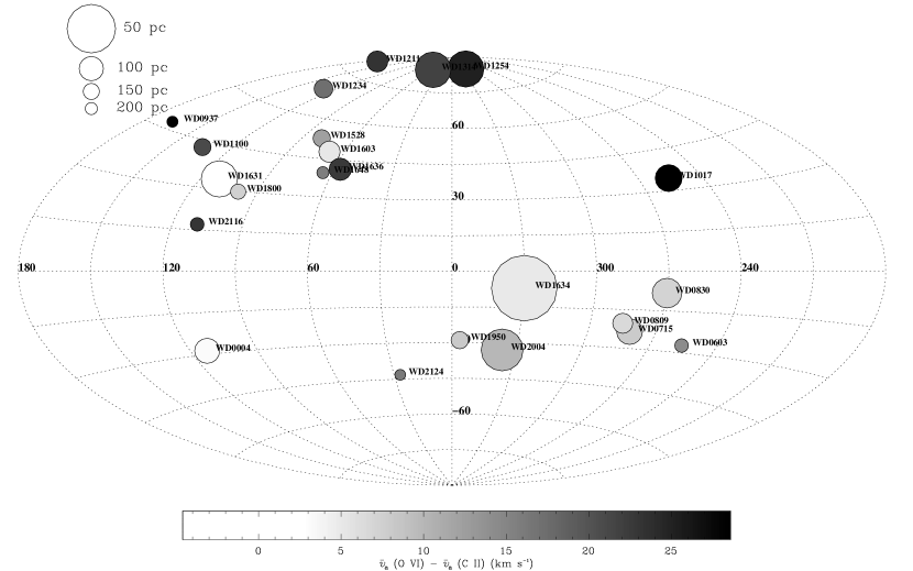
Figure 14: WD locations in Galactic coordinates ($l,b$) of the 24 stars from Table 5 except WD 0455$-$282 with $\geq 2\sigma$ O VI detections and not likely affected by stellar contamination. Same symbol code as Fig. 1 except the grey scale indicates $\Delta v=\bar{v}_{a}($O VI$)-\bar{v}_{a}($C II). Note that the WDs with the larger values of $\Delta v$ lie north of the Galactic plane.

References

- (1) Bannister, N. P., Barstow, M. A., Holberg, J. B., & Bruhweiler, F. C. 2003, MNRAS, 341, 477
- (2) Böhringer, H., & Hartquist, T. W. 1987, MNRAS, 228, 915
- (3) Borkowski, K. J., Balbus, S. A., Fristrom, C. C. 1990, ApJ, 355, 501
- (4) Bowen, D. V., Jenkins, E. B., Tripp, T. M., Sembach, K. R., & Savage, B. D. 2005, in ASP Conf. Ser. XX, Astrophysics in the Far-Ultraviolet, ed. G. Sonneborn, H.W.
- (5) Cox, D. P. 2005, ARAA, in press
- (6) Danforth, C. W., & Shull, J. M. 2005, ApJ, 624, 555
- (7) Davidsen, A. F. 1993, Science, 259, 327
- (8) Dreizler, S., & Werner, K. 1996, A&A, 314, 217
- (9) Dupree, A. K., & Raymond, J. C. 1983, ApJ, 275, L71
- (10) Edgar, R. J., & Chevalier, R. A. 1986, ApJ, 310, L27
- (11) Fang, T., Sembach, K. R., Canizares, C. R. 2003, ApJ, 586, L49
- (12) Feigelson, E. D., & Nelson, P. I. 1985, ApJ, 293, 192
- (13) Fields, B. D., Hochmuth, K. A., & Ellis, J. 2005, ApJ, 621, 902
- (14) Finley, D. S., Koester, D., & Basri, C. 1997, ApJ, 488, 375
- (15) Fitzpatrick, E. L., & Spitzer, L. 1997, ApJ, 475, 623
- (16) Fox, A. et al. 2004, ApJ, 602, 738
- (17) Fox, A. et al. 2005, ApJ, [astro-ph/0505299]
- (18) Futamoto, K. et al. 2004, ApJ, 605, 793
- (19) Grevesse, N. 1984, Phys. Scripta, T8, 49
- (20) Heckman, T. M., Norman, C. A., Strickland, D. K., & Sembach, K. R. 2002, ApJ, 577, 691
- (21) Holberg, J. B., Barstow, M. A., & Sion, E. M. 1998, ApJS, 119, 207
- (22) Hoopes, C. G., Sembach, K. R., Howk, J. C., Savage, B. D., & Fullerton, A. W. 2002, ApJ, 569, 233
- (23) Howk, J. C., Sembach, K. R., Savage, B. D., Massa, D., Friedman, S. D., & Fullerton, A. W. 2002, ApJ, 569, 214
- (24) Hurwitz, M., et al. 1998, ApJ, 500, L61
- (25) Isobe, T., Feigelson, E.D., & Nelson, P. I. 1986, ApJ, 306, 490
- (26) Indebetouw, R., & Shull, J. M. 2004, ApJ, 605, 205
- (27) Jenkins, E. B., & Meloy, D. A. 1974, ApJ, 193, L121
- (28) Jenkins, E. B. 1978a, ApJ, 219, 845
- (29) Jenkins, E. B. 1978b, ApJ, 220, 107
- (30) Knie, K. et al. 2004, Phys. Rev. Letters, 93, 171103
- (31) Kruk, J., et al. 2002, ApJS, 140, 19
- Lallement et al. (2003) Lallement, R., Welsh, B. Y., Vergely, J. L., Crifo, F., & Sfeir, D. 2003, A&A, 411, 447
- (33) Lehner, N. 2002, ApJ, 578, 126
- (34) Lehner, N., Jenkins, E. B., Gry, C., Moos, H. W., Chayer, P., & Lacour, S. 2003, ApJ, 595, 858
- (35) Linsky, J. L., Redfield, S., Wood, B. E., & Piskunov, N. 2000, ApJ, 528, 756
- (36) Linsky, J. L., & Wood, B. E. 1996, ApJ 463, 254
- Maíz-Apellániz (2001) Maíz-Apellániz, J. 2001, ApJ, 560, L83
- (38) McKernan, B., Yaqoob, T., & Reynolds, C. S. 2004, ApJ, 617, 232
- (39) Moos, H. W. et al. 2000, ApJ, 538, L1
- (40) Morton, D. C. 2003, ApJS, 149, 205
- (41) Napiwotzki, R., Hurwitz, M., Jordan, S., Bowyer, S., Koester, D., Weidemann, V., Lampton, M., & Edelstein, J. 1995, A&A, 300, L5
- (42) Nicastro, F. et al. 2002, ApJ, 573, 157
- (43) Oegerle, W. R. et al. 2000, ApJ, 538, L23
- (44) Oegerle, W. R., Jenkins, E. B., Shelton, R., Bowen, D. V., & Chayer, P. 2005, ApJ, 622, 377
- (45) Oliveira, C. M., Dupuis, J., Chayer, P., & Moos, H. W. 2005, ApJ, 625, 232
- (46) Otte, B., Murphy, E. M., Howk, J. C., Wang, Q. D., Oegerle, W. R., Sembach, K.R. 2003, ApJ, 591, 821
- (47) Perryman, M. A. C., et al. 1997, A&A, 323, L49
- (48) Redfield, S., & Linsky, J. L. 2000, ApJ, 534, 825
- (49) Redfield, S., & Linsky, J. L. 2002, ApJS, 139, 439
- (50) Redfield, S., & Linsky, J. L. 2004, ApJ, 602, 776
- (51) Richter, P., Savage, B. D., Tripp, T. M., Sembach, K. R. 2004, ApJS, 153, 165
- (52) Sahnow, D. S. et al. 2000, ApJ, 538, L7
- (53) Sankrit, R., & Blair, W. P. 2002, ApJ 565, 297
- (54) Sankrit, R., Blair, W. P., & Raymond, J. C. 2004, AJ 128, 1615
- (55) Savage, B. D. 1995, in ASP Conf. Ser. 80, The Physics of the Interstellar and Intergalactic Medium, ed. A. Ferrara, C. F. McKee, C. Heiles, & P. R. Shaprio (San Francisco:ASP), 233
- (56) Savage, B. D. et al. 2000, ApJ, 538, L27
- (57) Savage, B. D., Sembach, K. R., Tripp, T. M., & Richter, P. 2002, ApJ, 564, 631
- (58) Savage, B. et al. 2003, ApJS, 146, 125
- (59) Savage, B. D., Wakker, B. P., Fox, A. J., & Sembach, K. R. 2005, ApJ, 619, 863
- (60) Savage, B. D., & Sembach, K. R. 1991, ApJ, 379, 245
- (61) Sembach, K. R., & Savage, B. D. 1992, ApJS, 83, 147
- (62) Sembach, K. R. et al. 2000, ApJ, 538, L31
- (63) Sembach, K. R. et al. 2003, ApJS, 146, 165
- (64) Sembach, K. R. et al. 2004, ApJS, 155, 351
- (65) Sfeir, D. M., Lallement, R., Critfo, F., & Welsh, B. Y. 1999, A&A, 346, 785
- (66) Shelton, R. 2002, ApJ, 569, 758
- (67) Shelton, R., & Cox, D. P. 1994, ApJ, 434, 599
- (68) Shelton, R. et al. 2001, ApJ, 560, 730
- (69) Silvestri, N. M. et al. 2001, AJ, 121, 503
- (70) Slavin, J. D. 1989, ApJ, 346, 718
- Slavin & Cox (1993) Slavin, J. D., & Cox, D. P. 1993, ApJ, 417, 187
- (72) Smith, R. K., & Cox, D. P. 2001, ApJS, 134, 283
- (73) Snowden, S. L. et al. 1998, ApJ 493, 715
- (74) Spitzer, L. 1956, ApJ, 124, 20
- (75) Spitzer, L. 1990, ARAA, 28, 71
- (76) Sutherland, R. S., & Dopita, M. A. 1993, ApJS, 88, 253
- (77) Tripp, T. M., Savage, B. D., & Jenkins, E. B. 2000, ApJ, 534, L1
- (78) Van Altena, W. F., Lee, J. T., & Hoffeit, E. D. 1995, The General Catalog of Trigonometric Stellar Parallaxes (New Haven: Yale University Observatory)
- (79) Vennes, S., Thhejll, P.A., Wickramasinghe, D. T., & Bessell, M. S. 1996, ApJ, 467, 782
- (80) Vennes, S. et al. 1998, ApJ, 500, L41
- (81) Wakker, B. P. et al. 2003, ApJS, 146, 1
- (82) Welsh, B. Y., Sfeir, D. M., Sirk, M. M. & Lallement, R. 1999, A&A, 352, 308
- (83) Widmann, H. et al. 1998, A&A, 338, L1
- (84) Williamson, F. O., Sanders, W. T., Kraushaar, W., McCammon, D., Borken, R., & Bunner, A. N. 1974, ApJ, 193, L133
- (85) Wood, B. E. et al. 2002, ApJS, 140, 91
- (86) Wood, B. E., & Linsky, J. L. 1998, ApJ 492, 788
- (87) Yao, Y., & Wang, Q. D. 2005, ApJ, 625, 751
- (88) York, D. G. 1974, ApJ, 193, L127
- (89) Zsargó, J., Sembach, K. R., Howk, J. C., & Savage, B. D. 2003, ApJ, 586, 1019