Explosion Mechanism, Neutrino Burst, and Gravitational Wave in Core-Collapse Supernovae

Abstract

Core-collapse supernovae are among the most energetic explosions in the universe marking the catastrophic end of massive stars. In spite of rigorous studies for several decades, we still don’t understand the explosion mechanism completely. Since they are related to many astrophysical phenomena such as nucleosynthesis, gamma-ray bursts and acceleration of cosmic rays, understanding of their physics has been of wide interest to the astrophysical community.

In this article, we review recent progress in the study of core-collapse supernovae focusing on the explosion mechanism, supernova neutrinos, and the gravitational waves. As for the explosion mechanism, we present a review paying particular attention to the roles of multidimensional aspects, such as convection, rotation, and magnetic fields, on the neutrino heating mechanism. Next, we discuss supernova neutrinos, which is a powerful tool to probe not only deep inside of the supernovae but also intrinsic properties of neutrinos. For this purpose, it is necessary to understand neutrino oscillation which has been established recently by a lot of experiments. Gravitational astronomy is now also becoming reality. We present an extensive review on the physical foundations and the emission mechanism of gravitational waves in detail, and discuss the possibility of their detections.

1 Overview

Core-collapse supernovae are among the most energetic explosions in the universe. They mark the catastrophic end of stars more massive than 8 solar masses leaving behind compact remnants such as neutron stars or stellar mass black holes. Noteworthy, they have been thought to be extremely important astrophysical objects and thus have been of wide interest to the astrophysical community. The nucleosynthesis in these massive stars, and their subsequent explosions, are responsible for most of the heavy element enrichment in our galaxy. So naturally, any attempt to address human origins must begin with an understanding of core-collapse supernovae.

At the moment of explosion, most of the binding energy of the core is released as neutrinos. These neutrinos, which we call them as supernova neutrinos in the following, are temporarily confined in the core and escape to the outer region by diffusion. Thus supernova neutrinos will have valuable information of deep inside of the core. In fact, the detection of neutrinos from SN1987A paved the way for the Neutrino Astronomy, which is an alternative to the conventional astronomy by electromagnetic waves. Even though neutrino events from SN1987A were just two dozens, they have been studied extensively and allowed us to have a confidence that the basic picture of core-collapse supernova is correct.

Here it is worth mentioning that supernova neutrinos have attracted not only astrophysicist but also particle physicist. This is because supernova neutrinos are also useful to probe intrinsic properties of neutrinos as well as supernova dynamics. Conventionally they are used to set constraints on neutrino mass, lifetime and electric charge etc. More recent development involves neutrino oscillation, which have been established experimentally in the last decade. Neutrino oscillation on supernova neutrinos is important in two ways. First, since neutrino oscillation changes the event spectra, we cannot obtain the information on the physical state of the core without a consideration of neutrino oscillation. Second, since supernova has a distinct feature as a neutrino source compared with other sources such as the sun, atmosphere, accelerator and reactor, it also acts as a laboratory for neutrino oscillation.

Supernova is now about to start even another astronomy, Gravitational-Wave Astronomy. In fact, core-collapse supernovae have been supposed to be one of the most plausible sources of gravitational waves. Currently a lot of long-baseline laser interferometers such as GEO600, LIGO, TAMA300 and VIRGO are running and preparing for the first direct observation, by which the prediction by Einstein’s theory of General Relativity can be confirmed.

Astrophysicists have been long puzzled by the origins of the gamma-ray bursts since their accidental discovery in the late sixties. Some recent observations imply that the long-duration gamma-ray bursts are associated with core-collapse supernovae. In a theoretical point of view, the gamma-ray bursts are considered to be accompanied by the failed core-collapse supernovae, in which not the neutron star but the black hole is left behind. It is one of the most exciting issue to understand how the failed core-collapse supernovae can produce the observed properties of the gamma-ray bursts.

In order to obtain the understanding of these astrophysical phenomena related to core-collapse supernovae and the properties of neutrino and gravitational-wave emissions, it is indispensable to understand the explosion mechanism of core-collapse supernovae. However one still cannot tell it exactly albeit with the elaborate efforts during this 40 years. At present, detections of neutrinos and gravitational waves from nearby core-collapse supernovae are becoming reality. Since neutrinos and gravitational waves can be the only window that enables us to see directly the innermost part of core-collapse supernovae, their information is expected to help us to understand the explosion mechanism itself. Under the circumstances, the mutual understanding of the explosion mechanism, the supernova neutrinos, and the gravitational waves, which we will review in turn in this article, will be important.

The plan of this article is as follows. We begin by a brief description of the standard scenario of core-collapse supernovae in section 2. In section 3, we give a tool to discuss supernova neutrinos and their observation, neutrino oscillation. Although neutrino oscillation is thought to have only a negligible effect on the dynamics of supernova, it is necessary when we try to interpret observed neutrinos and extract information of supernova from them. Then supernova neutrinos and their neutrino oscillation are elaborately reviewed in section 4. With respect to the study of the explosion mechanism, good progress in the multi-dimensional models has been made recently. We review these studies in section 5. Finally, gravitational waves in core-collapse supernovae are reviewed in section 6, in which we pay a particular attention to the predicted characteristics of gravitational waves and their detectability for the currently running and planning laser interferometers. So far a number of excellent reviews already exist on various topics in this article. This article goes beyond such reviews to cover more the state-of-the-art investigations.

2 Supernova Theory

2.1 The Fate of Massive Star

In a historical view point, supernovae owe their name to astronomers Walter Baarde and Fritz Zwicky, who already in the early 1930’s realized that these objects show a sudden bursts in luminosity that slowly decays, similar to common novae, but much more luminous and rare [18]. Their high luminosities comparable to the integrated light of their host galaxies and their broad spectral lines led them to conclude that supernovae were very energetic explosions produced at the death of the massive star. What is amazing is that they suggested that a supernova derive their tremendous energy from gravitational collapse, in particular that the inner part of the star collapses to a neutron star. Although much observational and theoretical progress have been made since then, and many physical principles and important details have been identified, the basic picture of the early 1930’s still holds nowadays. To begin with, we review the current understanding of the fate of the massive stars in the following.

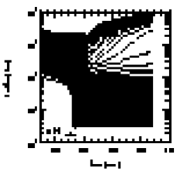
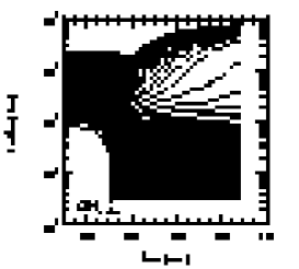
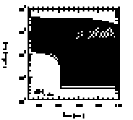
The fate of a single massive stars, that is to say, whether the remnant formed after stellar collapse will be a neutron star or a black hole, is mainly determined by its mass at birth and by the history of its mass loss during its evolution. The mass loss is expected to be crucially affected by the initial metalicity of the star, because the mass loss rate by the stellar winds is sensitive to the photon opacity, which is determined by the metalicity. The stars with high initial metalicity have more mass loss, and thus, have smaller helium cores and hydrogen envelopes during its evolution. Stellar collapse of such stars tends to lead to the formation of a neutron star, while for the lower metalicity stars, a black hole [123]. Figure 1 illustrates how the remnants of massive stars will be as a function of the initial mass and the metalicity (this figure is taken from [123]). From the figure, stellar collapse of the stars with the initial masses above $\sim 9M_{\odot}$ and below $\sim 25M_{\odot}$ lead to the formation of neutron stars. Above $25M_{\odot}$, black holes are expected to be formed either by fall-back of matter after the weak explosion (below $40M_{\odot}$) or directly if the stellar core is too massive to produce the outgoing shock wave (above $40M_{\odot}$). Given a fixed initial mass above $40M_{\odot}$, the stars with smaller initial metalicity tend to form a black hole directly due to the more heavier core as a result of the less mass-loss activities during evolution.

Recently, the fate of massive stars has been paid considerable attention. This is mainly due to the accumulating observations that the death of massive stars and supernova-like events are associated with the long-duration gamma-ray bursts (GRBs) (see, for example, [194]). The fact that accompanying supernovae are in general more energetic (they are frequently referred to as “hypernovae” in the literature) than the canonical core-collapse supernovae is another reason for this frenzy [225]. According to the most widely accepted theoretical models, it is believed that a black hole/an accretion disk system supported by the sufficient angular momentum is required [220]. In addition to the rapid rotation, the strong magnetic fields, as high as $10^{15}\sim 10^{16}$ G in the central regions are also pointed out to be helpful for producing the GRBs. In order to determine the progenitor of the gamma-ray bursts, stellar rotation and magnetic fields should be taken into consideration. Such investigation has just begun [122]. In addition, the astrophysical details of the geometry or environment of the black hole/accretion system are currently hidden from us both observationally and computationally. Although these are open questions now, this situation may change in the near future with the development of gravitational-wave and neutrino observatories and more sophisticated astrophysical simulation capabilities (see [262] for a review).

Very massive stars between $140M_{\odot}\leq M\leq 260M_{\odot}$ with the smaller initial metalicity are considered to become unstable to the electron-positron pair-instability ($\gamma\gamma\rightarrow e^{+}e^{-}$) during its evolution, which lead to the complete disruption of the star. Recently, explosions of metal-poor stars have been paid great attention because such stars are related to the first stars (the so-called Population III stars) to form in the universe. So far two hyper metal-poor stars, HE0107-5240 [69] and HE1327-2326 [96], whose metalicity is smaller than $1/100000$ of the sun, have been discovered. They provided crucial clues to the star formation history [281] and the synthesis of chemical elements [341, 150] in the early universe. Furthermore, neutrino emissions and gravitational waves from such stars are one of the most exciting research issues.

In this review, we focus on the ordinary supernova which lead to the neutron star formation ($\sim 9M_{\odot}\leq M\leq 25M_{\odot}$ with the solar metalicity). As will be explained below, the most promising scenario of the explosion mechanism of such stars are the neutrino-heating explosion. After we shortly refer to the current status of the presupernova models in section 2.2 (for details, see, [364, 123]), we explain the scenario in section 2.3.

Figure 1: Remnants of massive single stars as a function of initial metalicity and initial mass. In the regions above the thick green line (for the higher initial metalicity), the hydrogen envelope is stripped during its evolution due to the active mass loss processes. The dashed blue line indicates the border of the regime of direct black hole formation. The white strip near the right lower corner indicates the occurrence of the pair-instability supernovae. In the white region on the left side at lower mass, the stellar cores do not collapse and end their lives as white dwarfs. This figure is taken from Heger et al (2003) [123].

2.2 Presupernova Models

Figure 2: Structure of the precollapse star (Woosley and Weaver’s 15 $M_{\odot}$ model taken from [362]). In the upper panel, the temperature and density profiles are given. $L_{\rm tot}$, $\epsilon_{\nu}$, and $\epsilon_{\rm nuc}$, represents the total energy loss and the contribution from the neutrino emission and from the nuclear-energy generation, respectively. In the lower panel, the composition profile is given.

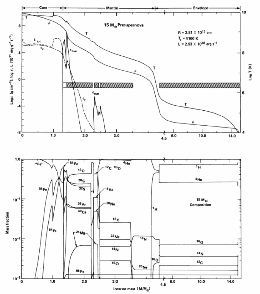
In Figure 2, an example of the precollapse stellar model by Woosley and Weaver (1995) [363], which has been often employed as an initial condition of core-collapse simulations, is shown. The iron core is surrounded by shells of lighter elements (the bottom panel of Figure 2). This is called onion-skin structure. The size of iron core is the order of $10^{9}$ cm while the stellar radius is larger than $10^{13}$ cm. At the core and the surrounding shell, the density decreases steeply and hence the dynamical timescale of the core (:$\tau_{\rm dyn}\sim(G\bar{\rho})^{-1/2}$ with $G$ and $\bar{\rho}$ being the gravitational constant and the average density) is much shorter than that of the envelope (see the upper panel of Figure 2). That is, the dynamics of the iron core is not affected by the envelope. Therefore we focus on the core hearafter for a while.

The late evolutional stage of massive stars are strongly affected by weak interactions. In fact, it can be seen from the upper panel of Figure 2 that the dominant energy loss process in the iron core is the neutrino emissions (see $L_{\rm tot}$, $\epsilon_{\nu}$, and $\epsilon_{\rm nuc}$ in the panel). The generated neutrinos, which are well transparent for densities $\bar{\rho}\leq 10^{11}~{}\rm{g}~{}\rm{cm}^{-3}$, escape the star carrying away energy and thus cooling the star. Due to the weak interactions, namely electron capture and beta decay, not only the core entropy $s$, but also the electron fraction $Y_{e}$, which is the electron to baryon ratio, changes. Since the mass of the presupernova core can be approximately expressed by the effective Chandrasekar mass [66, 334],

$$M_{\rm Ch}=5.83\bar{Y}_{e}^{2}\Bigl{[}1+\Bigl{(}\frac{\bar{s}_{e}}{\pi\bar{Y}_{e}}\Bigr{)}^{2}\Bigr{]}M_{\odot},$$ (1)

with $\bar{Y}_{e}$ and $\bar{s}_{e}$ being the average values of electron fraction and electronic entropy per baryon in the core, the weak interaction rates play an important role of determining the core mass. Putting the typical values of $\bar{Y}_{e}=0.45,\bar{s}_{e}=0.52$ in a $15M_{\odot}$ star into Eq. (1), one has an Chandrasekhar mass of $1.34M_{\odot}$ which is close to the core mass obtained by the stellar evolution calculation (see Figure 2).

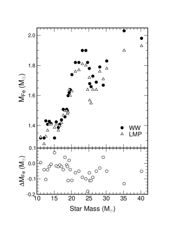
So far presupernova models have been constructed by employing the weak interaction rates by Fuller, Fowler and Newman (FFN) [104, 105, 106] for electron-capture rates with an older set of beta decay rates. As well known, the electron capture and its inverse are dominated by Fermi and Gamow-Tellar transitions. A correct description of the Gamow-Tellar transitions is difficult because it requires to solve the many-body problem in the nuclear structure. Due to the restricted available experimental data in the mid 1980’s, the tabulations of FFN could not fully describe the Gamow-Taylor distributions in nuclei. This has been practicable recently by the new-shell model calculation by Langanke and Martínez-Pinedo ([189, 190], see [193] for review). According to Heger et al [124, 125], who studied the effect of the shell model rates on presupernova models by repeating the calculations of Woosley and Weaver (1995) [363] while fixing the other stellar physics, the iron core mass is found to be reduced about up to $0.2M_{\odot}$ than the ones in Woosley and Weaver’s computations (see Figure 3).

Figure 3: Comparison of the values of the iron core masses for $11-40M_{\odot}$ stars between the Woosley and Weaver’s models (WW) using the FFN interaction rates and the ones using the shell model weak interaction rates by Langanke and Martínez-Pinedo (LMP) [189, 190]. $\Delta M_{\rm Fe}$ represents the difference of the masses between the two computations. This figure is taken from [193].

2.3 Standard Scenario of Core-collapse Supernova Explosion

In the following, we shall briefly outline the modern picture of the explosion mechanism of core-collapse supernovae (see, also [35, 319] for reviews).

2.3.1 onset of infall

In the late-time iron core of a massive star, the pressure, which supports it against the core’s own gravitational force, is dominated by a degenerate gas of relativistic electrons,

$$P_{\rm e}=\frac{1}{4}(3\pi^{2})^{1/3}\Bigl{(}\frac{\rho}{m_{u}}\Bigr{)}^{4/3}Y_{\rm e}^{4/3},$$ (2)

where $Y_{\rm e}\equiv n_{e^{-}}-e_{e^{+}}$ is electron fraction per baryon, $m_{u}$ is the atomic mass unit, and $\rho$ is the density. At the typical core densities and temperatures ($\rho\sim 10^{10}~{}{\rm g}~{}{\rm cm}^{-3}$ and $T\sim 10^{10}~{}{\rm K}$), the electron capture on Fe nuclei occurs via

$${}^{56}{\rm Fe}+e^{-}\rightarrow{}^{56}{\rm Mn}+\nu_{e},$$ (3)

because the Fermi energy of electrons,

$$\mu_{e} = (3\pi^{2}n_{e})^{\frac{1}{3}}\hbar c$$ (4)

$$= 11.1{\rm MeV}\left(\frac{\rho Y_{e}}{10^{10}{\rm g}~{}{\rm cm}^{-3}}\right)^{\frac{1}{3}}$$ (5)

exceeds the mass difference between the nuclei, namely, $m_{\rm Mn}-m_{\rm Fe}=3.7{\rm MeV}$. Decrease of the electron fraction results in the reduction of the pressure support and the core begins to collapse. Note that neutrinos escape freely from the core before the central density for $\rho\lesssim 10^{11}{\rm g}~{}{\rm cm}^{-3}$ as will be mentioned in the next subsection.

The onset of core-collapse can be also understood by the fact that the adiabatic index:

$$\Gamma_{S}\equiv\left(\frac{\partial\ln p}{\partial\ln\rho}\right)_{S},$$ (6)

is lowered below $4/3$, which is the instability condition against the radial perturbation of a spherical star [66]. From Eq. (2), the adiabatic index becomes

$$\Gamma_{S} = \left.\frac{\partial\ln{P_{e}}}{\partial\ln{\rho}}\right|_{S}=\left.\frac{\partial\ln{P_{e}}}{\partial\ln{\rho}}\right|_{S,Y_{e}}+\left.\frac{\partial\ln{Y_{e}}}{\partial\ln{\rho}}\right|_{S}\left.\frac{\partial\ln{P_{e}}}{\partial\ln{Y_{e}}}\right|_{S}+\left.\frac{\partial\ln{S}}{\partial\ln{\rho}}\right|_{Y_{e}}\left.\frac{\partial\ln{P_{e}}}{\partial\ln{S}}\right|_{Y_{e}}$$ (7)

$$= \frac{4}{3}\left(1+\left.\frac{\partial\ln{Y_{e}}}{\partial\ln{\rho}}\right|_{S}\right),$$ (8)

where the final term on Eq.(7) is set to zero, because the collapse proceeds almost adiabatically. Progression of electron capture implies negative $\left.\frac{\partial\ln{Y_{e}}}{\partial\ln{\rho}}\right|_{S}$ which makes $\Gamma_{S}$ less than $4/3$.

Furthermore, the endothermic photodissociation of iron nuclei,

$$\gamma+^{56}{\rm Fe}\rightarrow 13\alpha+4n-124.4{\rm MeV}$$ (9)

occurs for the temperature $T\geq 5\times 10^{9}$ K, which leads to the reduction of the thermal pressure support. In addition, the internal energy produced by the core contraction is exhausted by this reaction. Both of them promote the core collapse.

Since the degenerate pressure of relativistic electrons in finite temperature can be expressed as,

$$P_{e}=\frac{\mu_{e}^{4}}{12\pi^{2}c^{3}\hbar^{3}}\Biggl{[}1+\frac{2}{3}\Bigl{(}\frac{S_{e}}{\pi Y_{e}}\Bigr{)}^{2}\Biggr{]},$$ (10)

the adiabatic index in Eq. (6) becomes,

$$\Gamma_{S}\approx\frac{4}{3}\Bigl{[}1+\frac{\alpha^{2}}{1+2/3\alpha^{2}}\left.\frac{\partial\ln{S_{e}}}{\partial\ln{\rho}}\right|_{Y_{e}}\Bigr{]},$$ (11)

where $S_{e}=\pi^{2}Y_{e}k_{\rm B}T/\mu_{e}$ is the electron entropy with $k_{\rm B}$ being the Boltzmann constant [30]. The electron entropy decreases with the central density during infall phase because the photodissociation proceeds by the loss of the thermal energy of electrons. Hence, $\left.\frac{\partial\ln{S_{e}}}{\partial\ln{\rho}}\right|_{Y_{e}}$ in Eq. (11) becomes negative, by which the core is shown to be destabilized by the reaction. It is noted that the entropy transfer from electron to nucleon occurs during the core collapsing phase because the reduction of electron entropy leads to the increase of the entropy of nucleons, while conserving the total entropy [30].

2.3.2 neutrino trapping

After the onset of gravitational collapse, the core proceeds to contract under the pull of the self gravitational force, unnoticed by the rest of the outer part of the star, on a free-fall time scale, which is of the order of $\tau\sim(G\bar{\rho})^{-1/2}\sim 0.04~{}{\rm sec}~{}(\bar{\rho}/1\times 10^{10}~{}{\rm g}~{}{\rm cm}^{-3})^{-1/2}$ with the average density of the core of $\sim 10^{10}~{}{\rm g}~{}{\rm cm}^{-3}$. When the central densities exceed $10^{11}-10^{12}~{}{\rm g}~{}{\rm cm}^{-3}$, electron neutrinos, which can escape freely from the core at first, begins to be trapped in the core, because the timescale for electron neutrino diffusion from the core becomes longer than that for the timescale of the core-collapse. This is the so-called “neutrino trapping” , which plays very important roles in supernova physics [278, 279, 97].

During the core collapses, only electron neutrinos ($\nu_{e}$) are produced copiously by electron captures. Since the wavelength of neutrinos with the typical energy of $E_{\nu}$,

$$\lambda\approx 20~{}{\rm fm}\Bigl{(}\frac{E_{\nu}}{10~{}{\rm MeV}}\Bigr{)}^{-1},$$ (12)

is longer than the size of the nuclei of ${}_{26}^{56}{\rm Fe}$,

$$r_{\rm nuc}\sim 1.2A^{1/3}~{}{\rm fm}\approx 5\left(\frac{A}{56}\right)^{\frac{1}{3}}{\rm fm},$$ (13)

neutrinos are scattered coherently off $A$ nucleons in the nucleus, by which the cross section ($\nu_{e}+A\rightarrow\nu_{e}+A$) becomes roughly $A^{2}$ times of the cross section of each scattering of nucleons ($\nu_{e}+n,p\rightarrow\nu_{e}+n,p$). Thus the coherent scattering of neutrinos is the dominant opacity source for the neutrinos during the infall phase.

The mean free path determined by the coherent scattering of the neutrinos on the iron nuclei is estimated to be,

$$\lambda_{\nu} = \frac{1}{\sigma_{A}~{}n_{A}},$$ (14)

where $n_{A}=\rho/(Am_{u})$ is the number density of nuclei and $\sigma_{A}$ is the cross section of the coherent scattering in the leading order (see the detailed one in [54]),

$$\sigma_{A}=\frac{1}{16}\sigma_{0}\Bigl{(}\frac{E_{\nu}}{m_{\rm e}c^{2}}\Bigr{)}^{2}A^{2}\Bigl{[}1-\frac{Z}{A}+(4\sin^{2}\theta_{w}-1)\frac{Z}{A}\Bigr{]}^{2},$$ (15)

where $\sigma_{0}=4G_{F}^{2}(m_{\rm e}c^{2})^{2}/(\pi(\hbar c)^{4})=1.705\times 10^{-44}~{}{\rm cm}^{2}$ is a convenient reference cross section of weak interactions, $G_{F}$ and $\theta_{w}$ is the Fermi coupling constant and the Weinberg angle. The mean electron-neutrino energy in the iron (${}_{26}^{56}{\rm Fe}$) core can be estimated as follows,

$$E_{\nu}\approx\frac{5}{6}\mu_{e}=\frac{5}{6}\left(3\pi^{2}\frac{\rho Y_{e}}{m_{u}}\right)^{\frac{1}{3}}\hbar c\approx 10.3{\rm MeV}\left(\frac{\rho}{3\times 10^{10}{\rm g}\;{\rm cm}^{-3}}\right)^{\frac{1}{3}}\left(\frac{Y_{e}}{26/56}\right)^{\frac{1}{3}}.$$ (16)

Introducing Eqs. (15) and (16) to Eq. (14), the mean free path in Eq. (14) becomes

$$\lambda_{\nu} = \frac{1}{\sigma_{A}~{}n_{A}}$$ (17)

$$= 8.5\times 10^{6}~{}{\rm cm}~{}\left(\frac{\rho}{3\times 10^{10}{\rm g}{\rm cm}^{-3}}\right)^{-1}\left(\frac{A}{56}\right)^{-1}\left(\frac{E_{\nu}}{10.3~{}{\rm MeV}}\right)^{-2},$$

$$\approx 10^{7}{\rm cm}\left(\frac{\rho}{3\times 10^{10}{\rm g}{\rm cm}^{-3}}\right)^{-5/3}\left(\frac{A}{56}\right)^{-1}\left(\frac{Y_{e}}{26/56}\right)^{-\frac{2}{3}}.$$ (18)

Since the mean free path becomes smaller than the size of the core,

$$R_{\rm core}\approx\Bigl{(}\frac{3M_{\rm core}}{4\pi\rho}\Bigr{)}^{1/3}\approx 2.7\times 10^{7}{\rm cm}\left(\frac{\rho}{3\times 10^{10}{\rm g}{\rm cm}^{-3}}\right)^{-\frac{1}{3}}\left(\frac{Y_{e}}{26/56}\right)^{\frac{2}{3}},$$ (19)

as the central density increases (note $\lambda_{\nu}\propto\rho^{-5/3}$, while $R_{\rm core}\propto\rho^{-1/3}$), neutrinos cannot escape freely from the core. This suggests that there is a characteristic surface determining the escape or trapping of neutrinos in the core. The radial position of the neutrino sphere is usually defined as the surface where the neutrino “optical” depth,

$$\tau(r,E_{\nu})=\int^{\infty}_{r}\frac{dr}{\lambda_{\nu}},$$ (20)

becomes $2/3$. The neutrino sphere is the effective radiating surface for neutrinos, in analogy with the “photosphere” of normal light emitting surface. It is noted that its position differs from neutrino species to species and is dependent on the neutrino energy. The neutrino sphere, which we are now discussing, is of the electron neutrinos defined by their mean energy.

Introducing Eq. (18) to the above equation, one obtains

$$\tau(r,E_{\nu})\propto E^{2}_{\nu}\int^{\infty}_{r}\rho(r)A(r)dr.$$ (21)

Taking the distribution of the density, which can be approximated by

$$\rho(r)=H\frac{1}{r^{3}}~{}~{}(~{}{\rm with}~{}H=3\times 10^{31})$$ (22)

during the collapsing phase [35], and taking the typical values of $A=56$ at the central density of $\rho=10^{12}~{}{\rm g}~{}{\rm cm}^{-3}$, the optical depth becomes

$$\tau(r,E_{\nu})\approx 6.1\left(\frac{E_{\nu}}{10{\rm MeV}}\right)^{2}\left(\frac{\rho(r)}{10^{12}{\rm g}\;{\rm cm}^{-3}}\right)^{\frac{2}{3}}.$$ (23)

Thus the typical radial position and the density of the neutrino sphere ($\tau(R_{\nu},E_{\nu})$ = 2/3) becomes

$$R_{\nu}\approx 1.0\times 10^{7}~{}{\rm cm}\left(\frac{E_{\nu}}{10{\rm MeV}}\right),$$ (24)

$$\rho(R_{\nu}(E_{\nu}))=3.6\times 10^{10}{\rm g}\;{\rm cm}^{-3}\left(\frac{E_{\nu}}{10{\rm MeV}}\right)^{-3}.$$ (25)

Neutrinos produced at $R>R_{\nu}$ can freely escape from the core, while neutrinos produced inside propagates outwards by a random-walk induced by the coherent scattering. The diffusion time for neutrinos to diffuse out from the core of size $R$, can be estimated as,

$$t_{\rm diff}=\frac{3R^{2}}{c\lambda_{\nu}}\approx 2.3\times 10^{-1}{\rm sec}\left(\frac{\rho}{10^{12}{\rm g}\;{\rm cm}^{-3}}\right).$$ (26)

Since the dynamical timescale of the core,

$$t_{\rm dyn}=4\times 10^{-3}{\rm sec}\left(\frac{\rho}{10^{12}{\rm g}\;{\rm cm}^{-3}}\right)^{-\frac{1}{2}},$$ (27)

is shorter for the core density of $10^{11}\sim 10^{12}{\rm g}\;{\rm cm}^{-3}$. This also means that neutrinos cannot freely escape from the core and trapped in the core. After the neutrino trapping, the lepton fraction ($Y_{l}=Y_{e}+Y_{\nu}$), where $Y_{\nu}=n_{\nu_{e}}-n_{\bar{\nu}_{e}}$ is the electron-type neutrino fraction per baryon, is kept nearly constant during the collapse stage. Furthermore, electron neutrinos also become degenerate like electrons and the $\beta-$ equilibrium is established between $e^{-}+p\rightarrow n+\nu_{e}$ and its inverse. After the achievement of the $\beta-$ equilibrium, the entropy is conserved and the collapse proceeds adiabatically.

2.3.3 homologous collapse

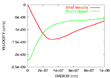
The collapsing core consists of two parts: the (homologously collapsing) inner core and the (supersonically infalling) outer core. This structure is clearly seen in Figure 4. Matter inside the sonic point (the point in the star where the sound speed equals the magnitude of the infall velocity) stays in communication and collapses homologously (velocity roughly proportional to radius). On the other hand, the material outside the sonic point falls in quasi-free fall with velocity proportional to the inverse square of the radius. Beautiful analytic studies have been done on this phase of collapse by [111, 365], who predict that the size of the homologous core is roughly the Chandrasekhar mass (see Eq. 1). For a typical value of $Y_{e}$ in the inner core, the mass of the inner core can be estimated $M_{\rm ch}\approx 0.5-0.8M_{\odot}$, which is in good agreement with the mass of the inner core obtained in a realistic numerical simulation [55].

Figure 4: Infall velocity and sound velocity versus radius at the central density of $10^{12}~{}{\rm g}~{}{\rm cm}^{-3}$ of a 15 $M_{\odot}$ progenitor model. The region inside and outside the sonic point ($R\approx 200$ km, at which the two curves cross) roughly corresponds to the inner core and the outer core, respectively.

2.3.4 core bounce

When nuclear densities are reached in the collapsing core ($\rho_{\rm c}\sim 3\times 10^{14}{\rm g}~{}{\rm cm}^{-3}$), repulsive nuclear forces halt the collapse of the inner core driving a shock wave into the outer core. As the shock propagates into the outer core with dissociating nuclei into free nucleons, the electron capture process $e^{-}+p\rightarrow n+\nu_{e}$ generates a huge amount of electron neutrinos just behind the shock. Before the shock arrives at the neutrino sphere, these electron neutrinos cannot escape in the hydrodynamical scale. Because these regions are opaque to the final state electron neutrinos and they are effectively trapped because their diffusion time is much longer than that for the shock propagation. As the shock waves move out in outer radius and pass through the neutrino sphere, the previously trapped electron neutrinos decouple from the matter and propagate ahead of the shock waves. This sudden liberation of electron neutrinos is called the neutronization burst (or “breakout” burst) (see the top panel of Figure 5).

Figure 5: The luminosities and root-mean-square energies of the neutrinos as a function of time. The results of the 13 $M_{\odot}$ model are drawn with dashed lines and the results of the 40 $M_{\odot}$ model with solid lines. The time is measure from the core bounce. This figure is taken from [199].

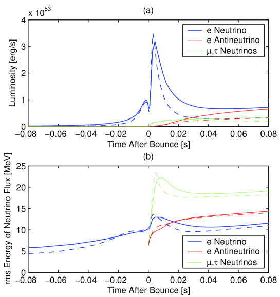
The duration of the neutronization burst is the timescale of the shock propagation and, hence, less than $\sim 20~{}{\rm msec}$. While the peak luminosity exceeds $10^{53}~{}{\rm erg}~{}{\rm s}^{-1}$, the total energy emitted in the neutronization burst is only of the order of $10^{51}~{}{\rm erg}$ due to the short duration timescale. This electron-neutrino breakout signal is expected to be detected from the Galactic supernova in modern neutrino detectors such as SuperKamiokande and the Sudbury Neutrino Observatory (see section 4).

The breakout of the electron neutrinos is almost simultaneous with the appearance of the other neutrino species. In the hot post-bounce region, the electron degeneracy is not high and relativistic positrons are also created thermally leading the production of anti-electron neutrinos ($\bar{\nu}_{e}^{\prime}~{}s$) via reaction $e^{+}+n\rightarrow p+\bar{\nu}_{e}$. Mu- and tau- neutrinos are also produced in this epoch by the electron-positron annihilation ($e^{+}e^{-}\rightarrow\nu_{\mu,\tau}\bar{\nu}_{\mu,\tau}$), nucleon-nucleon bremsstrahlung ($NN^{{}^{\prime}}\rightarrow NN^{{}^{\prime}}\nu_{\mu,\tau}\bar{\nu}_{\mu,\tau}$), and neutrino/anti-neutrino annihilation ($\nu_{e}\bar{\nu}_{e}\rightarrow\nu_{\mu,\tau}\bar{\nu}_{\mu.\tau}$) (see the bottom panel of Figure 5). Note that each process listed above also contributes for $\nu_{e}$ and $\bar{\nu}_{e}$ neutrinos, the production of these neutrinos are predominantly determined by the charged-current interactions, $e^{-}+p\rightarrow n+\nu_{e}$ and $e^{+}+n\rightarrow p+\bar{\nu}_{e}$.

At a radius of $100~{}{\rm km}\sim 200~{}{\rm km}$, the shock generated by core bounce stalls as a result of the following two effects. First, as the shock propagates outwards, it dissociates the infalling iron-peak nuclei into free nucleons, thus giving up $\sim 8.8~{}{\rm MeV}$ per nucleon in binding energy. Second, and most importantly, as the shock dissociates nuclei into free nucleons, electron capture on the newly-liberated protons to produce electron-neutrinos in the reaction $e^{-}+p\rightarrow n+\nu_{e}$.

Figure 6: Success or failure of the prompt explosion mechanism (courtesy of K. Sumiyoshi and see also [302, 303]). Each panel shows the trajectories of mass mesh in radius as a function of time for the different progenitor models. The number in the panels represents the mass of the progenitor models of $11,12,15,18,20M_{\odot}$ by [363] with the corresponding iron masses of $1.32,1.32,1.32,1.46,1.74M_{\odot}$. It can be seen that the prompt explosion mechanism works in the case of the relatively smaller progenitor mass with the smaller iron core.

Only for very special combinations of physical parameters, such as the stellar model of the progenitor or the incompressibility of nuclear matter, resulting in an extraordinary smaller cores, the so-called prompt explosion might work [130, 13, 131, 30], in which the shock wave at core bounce propagates through the outer core to produce explosions without the shock-stall (see Figure 6).

Figure 7: Successful of delayed explosion taken from [358]. The $x$ and $y$ axis represents the time in unit of second measured from core bounce and the radius from the stellar center in unit of centi-meter, respectively. Lines are trajectories of selected mass zones. The dashed line represents the shock front. 1.665 $M_{\odot}$ in the figure shows the mass point which is expelled outwards by the second shock due to the neutrino heating. As a result, the shock wave once weakened at $\sim 500$ msec revives and then successfully propagates to the surface of the iron core.

2.3.5 delayed explosion

Only several milliseconds after the shock-stall, a quasi-hydrostatic equilibrium is maintained between the newly-born protoneutron star (with radius of $\sim 50-80$ km) and the stalled accretion shock (with radius of $\sim 100-200$ km). The core of the protoneutron star is hot and dense, producing high-energy neutrinos of all species. If the energy transfer from the neutrinos to the material near the stalled shock is large enough, the stalled shock can be revived to produce the successful explosion. This neutrino-heating mechanism was discovered from the numerical simulations by Wilson [358] (see Figure 7). It is interesting to note that already in 1960’s, Colgate and White proposed that neutrino heating was essential for producing the explosions [72]. The amount of gravitational binding energy ($E_{\rm grav}$) released is huge,

$$E_{\rm kin}<<E_{\rm grav}\sim\frac{3}{5}\frac{GM_{\rm NS}^{2}}{R}\sim 3\times 10^{53}\Bigl{(}\frac{M_{\rm NS}}{1.4M_{\odot}}\Bigr{)}^{2}\Bigl{(}\frac{R_{\rm NS}}{10{\rm km}}\Bigr{)}^{-1}~{}{\rm erg},$$ (28)

in contrast to the kinetic energy of canonical observed supernovae ($E_{\rm kin}\sim 10^{51}$ erg), where $M_{\rm NS}$ and $R_{\rm NS}$ are the typical mass and the radius of a neutron star. Therefore in order to produce the explosions by the neutrino-heating mechanism, a small fraction ($\sim 1\%$) of the binding energy should be transfered, via neutrinos, to the mantle above the protoneutron star that is ejected as the supernova.

For the better understanding of the mechanism, we give an order-of-magnitude estimation according to [35, 154]. Let us assume the situation that a neutrino sphere is formed at radius of $R_{\nu}$ and from there, the isotropic neutrino with luminosity of $L_{\nu}$ is emitted (see Figure 8). Then the neutrino heating rate of nucleons via the reactions, $n+\nu_{e}\rightarrow e^{-}+p$ and $p+\bar{\nu_{e}}\rightarrow e^{+}+n$ at a radius $R$ ($R_{\nu}<R<R_{\rm s}$) can be estimated as,

$$Q_{\nu}^{+} \cong \frac{L_{\nu}~{}\sigma(\epsilon_{\nu})Y_{N}}{4\pi R^{2}}$$ (29)

$$\sim 53\Bigl{(}\frac{L_{\nu}}{10^{52}~{}{\rm erg}~{}{\rm s}^{-1}}\Bigr{)}\Bigl{(}\frac{\epsilon_{\nu}}{15~{}{\rm MeV}}\Bigr{)}^{2}\Bigl{(}\frac{R}{150~{}{\rm km}}\Bigr{)}^{-2}\Bigl{(}\frac{Y_{N}}{1.0}\Bigr{)}~{}\Bigl{[}\frac{\rm MeV}{{\rm s}\cdot{\rm nucleon}}\Bigr{]},$$

where $L_{\nu}$ is a typical neutrino luminosity, $\epsilon_{\nu}$ is the mean energy of neutrinos, $\sigma(\epsilon_{\nu})$ is the cross section of the above absorption processes. Here we take $Y_{N}$, the sum of the fraction of free nucleon and protons, to be $1$ because nuclei are nearly fully dissociated into free nucleons after the passage of the shock waves. Outside the stalled shock, on the other hand, the above heating rates are suppressed because of the absence of the free nucleons. Note that each value assumed in the above estimation is taken from the recent 1D core-collapse simulation [198].

Figure 8: Sketch of the stellar core during the shock revival phase. $R_{\nu}$ is the radius of neutrino sphere, from which neutrinos are emitted freely, $R_{\rm ns}$ is the radius of the protoneutron star, $R_{g}$ is the radius (see text) and $R_{s}$ is the radius of the stalled shock. The shock expansion is impeded by mass infall to the shock front at $R_{s}$ by the mass infall at a rate $\dot{M}$. This figure is taken from Janka (2001) [154].

On the other hand, the gravitational binding energy per baryon at a radius of $R$ can be given as follows:

$$-\frac{GM_{NS}m_{u}}{R}=-8.7\Bigl{(}\frac{M_{\rm NS}}{1.4M_{\odot}}\Bigr{)}\Bigl{(}\frac{R}{150{\rm km}}\Bigr{)}^{-1}~{}[{\rm MeV/nucleon}],$$ (30)

where we take $M_{NS}$ to be a typical mass scale of $1.4M_{\odot}$. Comparing the neutrino heating rate (r.h.s. of Eq. (29)) with the binding energy (r.h.s. of Eq. (30)), one can see that the neutrino heating can give the matter enough energy to be expelled from the core in 0.16 second. In realistic situations, the cooling of matter occurs simultaneously via the very inverse process of the heating reactions, which delays the timescale of the explosion up to $\sim 1~{}{\rm sec}$ [358]. These timescales are much longer than those of the prompt explosion mechanism ($O(10~{}{\rm msec})$). Thus the neutrino-driven mechanism is sometimes called as the delayed explosion mechanism.

Noteworthy, a characteristic radial position, which is the so-called gain radius, in which the neutrino heating and cooling balances and above which the neutrino heating dominates over the neutrino cooling, are formed after the shock-stall [33]. In the following, we estimate the position of the gain-radius by an order-of-magnitude estimation. In addition to the neutrino heating rate (Eq. (29)), the neutrino cooling rate of nucleons is given as follows:

$$Q_{\nu}^{-}=-\sigma(T)a^{{}^{\prime}}cT^{4},$$ (31)

where $T$ is the temperature of the material, $\sigma(T)$ is the corresponding neutrino absorption cross section, $a^{{}^{\prime}}=7/16\times 1.37\cdot 10^{26}~{}{\rm erg}~{}{\rm cm}^{-3}~{}{\rm MeV}^{4}$ is the radiation density constant of neutrinos, and $c$ is the speed of light. Since we assume for simplicity that the distribution function of neutrino is the fermi distribution with a vanishing chemical potential, then $a^{{}^{\prime}}T^{4}$ represents the energy density of neutrinos which yields to a black body radiation. Here we write $L_{\nu}$ in equation (29) as follows,

$$L_{\nu}=\pi R_{\nu}^{2}a^{{}^{\prime}}cT_{\nu}^{4},$$ (32)

assuming again that the neutrinos from the neutrino sphere are a Fermi distribution of the temperature $T_{\nu}$ of the neutrino sphere. Noting that $\sigma(T)/\sigma(T_{\nu})=(T/T_{\nu})^{2}$, the net heating rate can be written,

$$Q_{\rm tot}=Q_{\nu}^{+}-Q_{\nu}^{-}=Q_{\nu}^{+}\Biggl{[}1-\Bigl{(}\frac{2R}{R_{\nu}}\Bigr{)}^{2}\Bigl{(}\frac{T}{T_{\nu}}\Bigr{)}^{6}\Biggr{]}.$$ (33)

Using the simple power law relation,

$$T=T_{\rm s}\frac{R_{s}}{R},$$ (34)

which yields a good approximation in the radiation dominated atmosphere $R_{\nu}<R<R_{\rm s}$ [154], the position of the gain radius $R_{g}$ becomes

$$R_{g}=\sqrt{\frac{(2R_{s})^{3}}{R_{\nu}}\Bigl{(}\frac{T_{s}}{T_{\nu}}\Bigr{)}^{3}}.$$ (35)

Taking data obtained from a state-of-the-art numerical simulations [198], namely, $T_{\nu}=4.8{\rm MeV},T_{s}=1{\rm MeV},R_{s}=200{\rm km},R_{\nu}=80{\rm km}$, the gain radius becomes $85$ km, which is in good agreement with the position numerically obtained by the corresponding simulations (see Figure 9).

Figure 9: Heating and cooling rates by electron (left) and anti-electron (right) neutrinos at 100 msec after core bounce taken from Liebendörefer et al. 2001 [198]. At the moment, the neutrino sphere defined by its mean energy and the stalled shock is located at $R_{\nu}\sim 80$ km and $R_{s}\sim 200$ km, respectively. In both panels, dashed lines with positive values, dashed lines with negative lines, and solid lines represent the heating rates, cooling rates, and the net rates, respectively. From the figures, it is shown that the location where the net heating changes sign defines the gain radius $R_{g}\sim 80\sim 100$ km. Lines labeled by “NR” or “GR” indicate that the results are obtained by the Newtonian or general relativistic simulations.

The extent of the region of the net neutrino heating and the magnitude of the net neutrino energy deposition are responsible for producing the successful explosions and dependent crucially on the neutrino energy density and the flux outside the neutrino sphere, in which the neutrino semi-transparently couples to the matter. Thus the accurate treatment of neutrino transport is an important task in order to address the success or failure of the supernova explosions in numerical simulations.

If the neutrino heating mechanism works sufficiently to revive the stalled shock wave, the shock wave goes into the stellar envelope and finally blows off. This is observed as a supernova after the shock breaks out the photosphere. Unlike the case in the iron core, the photodissociation and the energy loss due to neutrinos is negligible in the stellar envelope and the binding energy is small, the shock wave successfully explodes the whole star. The propagation time of the shock wave depends on the stellar radius and is in the range from several hours to days.

Here we shall mention that there is another type of supernovae, driven by a quite different physical mechanism. Supernovae Type Ia characterized by the absence of hydrogen lines in their spectra are thought to be caused by a thermonuclear explosion of a white dwarf that is completely disrupted in this event (for a review of SN Ia explosion models see [132]). Since the luminosities at the explosions of Type Ia supernovae are almost constant, they are good candidates to determine extragalactic distances and to measure the basic cosmological parameters. We will not consider them in this review. Supernovae we pay attention to in this thesis are the so-called Type II, Type Ib and Ic, (for the recent observational classifications of supernovae, see [117] for example.) For convenience, we have used the common name “core-collapse supernovae” for supernovae of Types II and Ib/c.

3 Neutrino Oscillation

In this section, we give a fundamental tool to discuss supernova neutrinos and their observation, neutrino oscillation. These topics have been seldom reviewed systematically so far. Starting from the physical foundation, we give an elaborate description of the neutrino oscillation, which has been established recently by a lot of experiments. Based on this, neutrino oscillations in supernovae are reviewed in the next section.

3.1 Overview

So far, we know three types of neutrino, $\nu_{e},\nu_{\mu}$ and $\nu_{\tau}$. These are partners of the corresponding charged leptons, electron, muon and tauon, respectively, and produced via charged current interactions such as $\beta$-decay and decays of muons and tauons. Thus, $\nu_{e},\nu_{\mu}$ and $\nu_{\tau}$ are called flavor (weak) eigenstates, which mean the eigenstates of the weak interaction. On the other hand, we can also consider eigenstates of their free Hamiltonian. They are called mass eigenstates denoted as $\nu_{i}(i=1,2,3)$ and have definite masses $m_{i}$.

These types of eigenstates come from essentially different physical concept so that they do not necessarily coincide with each other. In fact, this is the case with the quark sector: Flavor eigenstates are linear combinations of mass eigenstates which are determined by a unitary matrix called Cabbibo-Kobayashi-Maskawa matrix. Then, like the quark sector, it is natural to consider that the leptons are also mixing.

The lepton mixing means that, for example, $\nu_{e}$, which is produced by $\beta$-decay, is a linear combination of some mass eigenstates $\nu_{i}$. More generally, neutrinos are always produced and detected in flavor eigenstates, which are not eigenstates of the propagation Hamiltonian. This mismatch leads to neutrino oscillation.

Neutrino oscillation can be roughly understood as follows. Expressing the wave function of the neutrino by plane wave, each mass eigenstate evolves as $\exp{[i(E_{i}t-\vec{k}_{i}\cdot\vec{x})]}$, where $E_{i}$ and $\vec{k}_{i}$ are energy and momentum of the mass eigenstate $\nu_{i}$. Because different masses $m_{i}^{2}$ lead to different dispersion relations $E_{i}^{2}=k_{i}^{2}+m_{i}^{2}$, phase differences between the wave functions would appear as the neutrino evolves. Thus time-evolved wave function of a flavor eigenstate is no longer the original linear combination of mass eigenstates, which means that there is a probability that the neutrino is detected as a different flavor from the original flavor.

3.2 Vacuum Oscillation

Let us start with the Klein-Gordon equation neglecting the spin degree of freedom of neutrino, which is not important unless neutrino has large magnetic dipole moment. The equations of motion of the mass eigenstates in vacuum are

$$\left(\frac{\partial^{2}}{\partial t^{2}}-\nabla^{2}+M^{2}\right)\Psi^{\rm(m)}=0,$$ (36)

where $\Psi^{\rm(m)}=(\nu_{1},\nu_{2},\nu_{3})$ is a wave-function vector of the mass eigenstates and $M={\rm diag}(m_{1},m_{2},m_{3})$ is the mass matrix. Let us expand the wave function as

$$\Psi^{\rm(m)}(t,\vec{x})=e^{-iEt}\Psi_{E}^{\rm(m)}(\vec{x}),$$ (37)

where we assumed all the mass eigenstates have the same energy $E$. Although this assumption is not physically appropriate, the results below are not affected if the neutrino is ultra-relativistic. Then the equations of motion become

$$\left(-E^{2}-\nabla^{2}+M^{2}\right)\Psi_{E}^{\rm(m)}=0$$ (38)

If the neutrino is ultra-relativistic $(E\sim k_{i}\gg m_{i})$, we have

$$-E^{2}-\nabla^{2}=-(E+i\nabla)(E-i\nabla)\approx-(E+i\nabla)2E,$$ (39)

which leads to

$$i\frac{\partial}{\partial z}\Psi_{E}^{\rm(m)}=-\left(E-\frac{M^{2}}{2E}\right)\Psi_{E}^{\rm(m)},$$ (40)

where we set the direction of motion to $z$ direction. The first term on the r.h.s. of Eq. (40) is irrelevant for neutrino oscillation because it just contributes to overall phase and will be neglected from now on.

On the other hand, flavor eigenstates can be written as linear combinations of mass eigenstates as,

$$\Psi_{E}^{\rm(f)}=U\Psi_{E}^{\rm(m)},$$ (41)

where $U$ is the mixing matrix, which is also referred to as the Maki-Nakagawa-Sakata (MNS) matrix [216]. This matrix corresponds to the Kobayashi-Maskawa matrix in the quark sector and often parameterized as,

$$U=\left(\begin{array}[]{ccc}c_{12}c_{13}&s_{12}c_{13}&s_{13}e^{-i\delta}\\ -c_{23}s_{12}-c_{12}s_{23}s_{13}e^{i\delta}&c_{12}c_{23}-s_{12}s_{23}s_{13}e^{i\delta}&c_{13}s_{23}\\ s_{12}s_{23}-s_{13}e^{i\delta}&-c_{12}s_{23}-c_{23}s_{12}s_{13}e^{i\delta}&c_{13}c_{23}\end{array}\right)$$ (42)

where $s_{ij}\equiv\sin{\theta_{ij}}$ and $c_{ij}\equiv\cos{\theta_{ij}}$, $\theta_{ij}(ij=1,2,3)$ are mixing angles and $\delta$ is $CP$ phase. In terms of the flavor eigenstates, the equations of motion (40) are expressed as,

$$i\frac{\partial}{\partial z}\Psi_{E}^{\rm(f)}=\frac{UM^{2}U^{{\dagger}}}{2E}\Psi_{E}^{\rm(f)}.$$ (43)

Here it should be noted that the mass matrix for flavor eigenstates, $UMU^{{\dagger}}$, is not diagonal in general.

As a simple example, let us assume that there are only two neutrino species, $\nu_{e}$ and $\nu_{\mu}$. Then the mixing matrix can be written as,

$$U=\left(\begin{array}[]{cc}\cos{\theta}&\sin{\theta}\\ -\sin{\theta}&\cos{\theta}\end{array}\right)$$ (44)

and the equations of motion reduce to

$$i\frac{\partial}{\partial z}\left(\begin{array}[]{c}\nu_{1}\\ \nu_{2}\end{array}\right)=\left(\begin{array}[]{cc}\frac{m_{1}^{2}}{2E}&0\\ 0&\frac{m_{2}^{2}}{2E}\end{array}\right)\left(\begin{array}[]{c}\nu_{1}\\ \nu_{2}\end{array}\right)$$ (45)

for mass eigenstates and

$$i\frac{\partial}{\partial z}\left(\begin{array}[]{c}\nu_{e}\\ \nu_{\mu}\end{array}\right)=\frac{\Delta m^{2}}{4E}\left(\begin{array}[]{cc}-\cos{2\theta}&\sin{2\theta}\\ \sin{2\theta}&\cos{2\theta}\end{array}\right)\left(\begin{array}[]{c}\nu_{e}\\ \nu_{\mu}\end{array}\right)$$ (46)

for flavor eigenstates. Here $\Delta m^{2}\equiv m_{2}^{2}-m_{1}^{2}$ and we again neglected a term proportional to identity matrix. Then consider a neutrino which is purely electron-type at first. Noting that electron-type neutrino can be written in terms of mass eigenstates as,

$$|\nu_{e}\rangle=\cos{\theta}|\nu_{1}\rangle+\sin{\theta}|\nu_{2}\rangle,$$ (47)

the neutrino evolves according to,

$$|\nu(z)\rangle=\exp{\left(-i\frac{m_{1}^{2}}{2E}z\right)}\cos{\theta}|\nu_{1}\rangle+\exp{\left(-i\frac{m_{2}^{2}}{2E}z\right)}\sin{\theta}|\nu_{2}\rangle.$$ (48)

Multiplying $\langle\nu_{e}|$, we obtain the probability that this state is electron type,

$$P_{\nu_{e}\rightarrow\nu_{e}}(z)=\left|\langle\nu_{e}|\nu(z)\rangle\right|^{2}=1-\sin^{2}{2\theta}\sin^{2}{\left(\pi\frac{z}{\ell_{\rm osc}}\right)},$$ (49)

where

$$\ell_{\rm osc}\equiv\frac{4\pi E}{\Delta m^{2}}=2.48\times 10^{7}{\rm cm}\left(\frac{E}{1{\rm MeV}}\right)\left(\frac{10^{-5}{\rm eV}}{\Delta m^{2}}\right)$$ (50)

is called the oscillation length. It is easy to show that

$$P_{\nu_{\mu}\rightarrow\nu_{e}}(z)=P_{\nu_{e}\rightarrow\nu_{\mu}}(z)$$ (51)

$$P_{\nu_{e}\rightarrow\nu_{e}}(z)=P_{\nu_{\mu}\rightarrow\nu_{\mu}}(z)=1-P_{\nu_{e}\rightarrow\nu_{\mu}}(z)$$ (52)

as expected by unitarity.

Figure 10: Conversion probability $P_{\nu_{e}\rightarrow\nu_{\mu}}(z)$ as a function of propagation distance $z$ normalized by the oscillation length $\ell_{\rm osc}$

The probability $P_{\nu_{e}\rightarrow\nu_{\mu}}(z)$ as a function of propagation distance $z$ is plotted in Fig. 10. It oscillates with respect to $z$ and the wave length is the oscillation length $\ell_{\rm osc}$. Here it will be worth noting that the oscillation length depends on the neutrino energy and the mass difference of the two involved mass eigenstates as is seen in (50). The amplitude is determined by the mixing angle and is the largest when $\theta=\pi/4$. Thus even if a neutrino is produced as an electron-type neutrino, there is non-zero probability that it is detected as a muon-type neutrino if there is a mixing between the two neutrino flavors. It is this phenomenon which is known as the neutrino oscillation.

Let us consider a more general case with many neutrino species. A neutrino state with a flavor $\alpha$ can be written as a linear combination of the mass eigenstates,

$$|\nu_{\alpha}\rangle=\sum_{i}U^{*}_{\alpha i}|\nu_{i}\rangle.$$ (53)

Then the evolution of a neutrino which is originally $\nu_{\alpha}$ is

$$|\nu(z)\rangle=\sum_{i}U^{*}_{\alpha i}\exp{\left(-i\frac{m_{i}^{2}}{2E}z\right)}|\nu_{i}\rangle,$$ (54)

and the probability $P_{\nu_{\alpha}\rightarrow\nu_{\beta}}(z)$ is

$$P_{\nu_{\alpha}\rightarrow\nu_{\beta}}(z)=\sum_{i}|U_{\alpha i}U_{\beta i}|^{2}+2{\rm Re}\sum_{i>j}U^{*}_{\alpha i}U_{\beta i}U_{\alpha j}U^{*}_{\beta j}\exp{\left(-i\frac{\Delta m_{ij}^{2}}{2E}z\right)}$$ (55)

where $\Delta m_{ij}^{2}\equiv m_{i}^{2}-m_{j}^{2}$.

averages

Figure 11: Conversion probability $P_{\nu_{e}\rightarrow\nu_{\mu}}(z)$ averaged by taking the finite size of a source into account.

Figure 12: Conversion probability $P_{\nu_{e}\rightarrow\nu_{\mu}}(z)$ averaged by a Gaussian energy distribution.

Finally we consider two averages of the conversion probability concerned with the finite size of a source and a finite energy width.

A neutrino source is, in general, not point-like and has a finite size. For example, in the sun, there is a spherical neutrino source with a radius $\approx 10^{10}{\rm cm}$ [20]. In this case, the finite size will average the phase of the oscillation of the conversion probability. Denoting the source distribution as $f(z_{0})$, the conversion probability is given by

$$P_{\nu_{e}\rightarrow\nu_{\mu}}(z)=\sin^{2}{2\theta}\int dz_{0}f(z_{0})\sin^{2}{\left(\frac{\pi(z-z_{0})}{l_{\rm osc}}\right)},$$ (56)

where $z$ is the distance between the center of the source and the detector. If we assume a Gaussian distribution with a width of $s$, that is,

$$f(z_{0})=\frac{1}{s\sqrt{2\pi}}e^{-\frac{z_{0}^{2}}{2s^{2}}},$$ (57)

the conversion probability is computed as,

$$P_{\nu_{e}\rightarrow\nu_{\mu}}(z)=\frac{1}{2}\sin^{2}{2\theta}\left[1-e^{-\frac{2\pi^{2}s^{2}}{l_{\rm osc}^{2}}}\cos{\left(\frac{2\pi z}{l_{\rm osc}}\right)}\right],$$ (58)

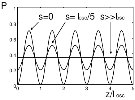
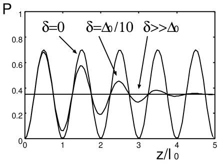
and is shown in Fig. 12. As one can see, if a source has a finite size, the amplitude of the probability oscillation become small while the average value remains unchanged. In the limit of $s\rightarrow 0$, it reduces to Eq. (49) and the oscillation is completely smoothed for $s\gg\ell_{\rm osc}$.

Next, let us consider a finite energy width. If a source has a finite energy width we must also average the conversion probability by the energy spectrum because the oscillation length (50) depends on neutrino energy:

$$P_{\nu_{e}\rightarrow\nu_{\mu}}(z)=\sin^{2}{2\theta}\int dEg(E)\sin^{2}\left(\frac{\Delta(E)z}{2}\right),$$ (59)

$$\Delta(E)\equiv\frac{2\pi}{l_{\rm osc}(E)}=\frac{\Delta m^{2}}{2E},$$ (60)

where $g(E)$ is the energy spectrum of neutrinos. As a simple example, we consider a spectrum with Gaussian $\Delta(E)$:

$$g(E)=\frac{1}{\delta\sqrt{2\pi}}e^{-\frac{(\Delta-\Delta_{0})^{2}}{2\delta^{2}}},~{}~{}~{}\Delta_{0}\equiv\frac{2\pi}{l_{0}(E)}=\frac{\Delta m^{2}}{2E_{0}},$$ (61)

where $\delta$ is the width and $E_{0}$ is the central energy. Here it should be noted that this distribution is not Gaussian with respect to neutrino energy. Then we have an averaged conversion probability,

$$P_{\nu_{e}\rightarrow\nu_{\mu}}(z)=\frac{1}{2}\sin^{2}{2\theta}\left[1-e^{-\frac{\delta^{2}z^{2}}{2}}\cos{\left(\frac{2\pi z}{l_{0}}\right)}\right].$$ (62)

This is plotted in Fig. 12. Although the oscillation is smoothed as in the case of the finite-size source, the behavior is different between the two cases. Since difference in energy leads to difference in oscillation length, the phase difference of two neutrinos with different energies increases as they propagate a long distance. Therefore, the conversion probability will cease to oscillate in the end regardless of the magnitude of the energy width.

3.3 Oscillation in Matter

The behavior of the neutrino oscillation changes if the neutrino propagates in the presence of matter, not in vacuum. Due to the interaction with matter, neutrino gains effective mass, which modifies the dispersion relation. If the interaction is flavor-dependent, like that with electrons, the change of the dispersion relation is also flavor-dependent. Remembering that the neutrino oscillation in vacuum is induced by different dispersion relations due to different masses, it is easy to imagine that further change in dispersion relations will change the behavior of the neutrino oscillation. This effect, the MSW effect, was first pointed out by Wolfenstein [353, 354] and discussed in detail by Mikheyev and Smirnov [226, 227, 228]. As will be discussed below, if matter is homogeneous, the situation is essentially the same as the vacuum oscillation with effective mixing angles determined by matter density and the original mixing angles.

What is interesting and important is a case with varying density. In fact, the MSW effect with varying density gave the solution to the long-standing solar neutrino problem [314, 298] and will also play a important role in supernovae.

3.3.1 constant density

At low energies only the elastic forward scattering is important and it can be described by the refraction index $n_{\rm ref}$. In terms of the forward scattering amplitude $f(E)$, the refraction index is written as

$$n_{\rm ref}=1+\frac{2\pi n}{E^{2}}f(E),$$ (63)

where $n$ is the target density. Then we have the dispersion relation in matter as

$$(n_{\rm ref}E)^{2}=k^{2}+m^{2}.$$ (64)

If we rewrite this dispersion relation as

$$(E-V_{\rm eff})^{2}=k^{2}+m^{2},$$ (65)

we obtain the effective potential $V_{\rm eff}$ as

$$V_{\rm eff}=(1-n_{\rm ref})E=-\frac{2\pi n}{E}f(E).$$ (66)

On the other hand, low-energy effective Hamiltonian for weak interaction between a neutrino and a target fermion is

$$H_{\rm int}=\frac{G_{F}}{\sqrt{2}}\bar{\psi}_{f}\gamma_{\mu}(C_{V}-C_{A}\gamma_{5})\psi_{f}\bar{\psi}_{\nu}\gamma^{\mu}(1-\gamma_{5})\psi_{\nu}$$ (67)

where $\psi_{f}$ is the target fermion field, $\psi_{\nu}$ is the neutrino. Here the coupling constant $G_{F}$ is the Fermi constant,

$$G_{F}=1.2\times 10^{-5}{\rm GeV}^{-2}=9\times 10^{-38}{\rm eV}~{}{\rm cm}^{3},$$ (68)

and $C_{V}$ and $C_{A}$ are vector weak charge and axial-vector weak charge, respectively, which depend on the species of the target. For the neutral-current interactions, charges are shown in Table 1 and for the charged-current interaction, $C_{V}=C_{A}=1$.

fermion	neutrino	$C_{V}$	$C_{A}$
electron	$\nu_{e}$	$1/2+2\sin^{2}{\theta_{\rm W}}$	$1/2$
	$\nu_{\mu,\tau}$	$-1/2+2\sin^{2}{\theta_{\rm W}}$	$-1/2$
proton	$\nu_{e,\mu,\tau}$	$1/2-2\sin^{2}{\theta_{\rm W}}$	$1.37/2$
neutron	$\nu_{e,\mu,\tau}$	$-1/2$	$-1.15/2$
neutrino($\nu_{\alpha}$)	$\nu_{\alpha}$	$1$	$1$
	$\nu_{\beta\not=\alpha}$	$1/2$	$1/2$

Table 1: Effective weak coupling constant for neutral-current interactions. Here $\theta_{\rm W}$ is the Weinberg angle $\sin^{2}{\theta_{\rm W}}\approx 0.23$.

Using the Hamiltonian and coupling constant, the forward scattering amplitude, refraction index and effective potential are computed as,

$$f(E)=\mp C^{\prime}_{V}G_{F}\frac{E}{2\sqrt{2}\pi},$$ (69)

$$n_{\rm ref}=1\mp C^{\prime}_{V}G_{F}\frac{n_{f}-n_{\bar{f}}}{\sqrt{2}E},$$ (70)

$$V_{\rm eff}=\pm C^{\prime}_{V}G_{F}\frac{n_{f}-n_{\bar{f}}}{\sqrt{2}}\equiv C^{\prime}_{V}G_{F}n_{B}\frac{Y_{f}}{\sqrt{2}},$$ (71)

for neutrino and anti-neutrino, respectively. Here $n_{B}$ is the baryon density, $n_{f}$ and $n_{\bar{f}}$ are fermion and anti-fermion number density, $Y_{f}\equiv(n_{f}-n_{\bar{f}})/n_{B}$ is the fermion number fraction per baryon and

$$C^{\prime}_{V}=\left\{\begin{array}[]{ll}C_{V}&(f\not=\nu)\\ 2C_{V}&(f=\nu)\end{array}\right..$$ (72)

Assuming charge neutrality ($Y_{e}=Y_{p}$), we have

$$V_{\rm eff}=\pm\sqrt{2}G_{F}n_{B}\times\left\{\begin{array}[]{ll}(-\frac{1}{2}Y_{n}+Y_{e}+2Y_{\nu_{e}})&({\rm for}\;\;\nu_{e})\\ (-\frac{1}{2}Y_{n}+Y_{\nu_{e}})&({\rm for}\;\;\nu_{\mu,\tau})\end{array}\right.$$ (73)

With this effective potential, the wave equation (43) is modified as

$$i\frac{\partial}{\partial z}\Psi_{E}^{\rm(f)}=\left[A+\frac{UM^{2}U^{{\dagger}}}{2E}\right]\Psi_{E}^{\rm(f)},$$ (74)

where $A$ is the mass matrix representing the contribution from interactions with matter. Neglecting the background neutrino, we have

$$A=\frac{G_{F}n_{B}}{\sqrt{2}}\left(\begin{array}[]{ccc}3Y_{e}-1&0&0\\ 0&Y_{e}-1&0\\ 0&0&Y_{e}-1\end{array}\right).$$ (75)

Here we used $Y_{n}=1-Y_{p}=1-Y_{e}$ but the contribution from neutrons is not important for neutrino oscillation because it is proportional to identity matrix. This reflects the fact that the interaction with neutrons is via the neutral-current interaction which occurs equally to all flavors.

Again, let us consider the two-flavor case. The wave equation in matter (74) can be rewritten as

$$i\frac{\partial}{\partial z}\left(\begin{array}[]{c}\nu_{e}\\ \nu_{\mu}\end{array}\right)=\frac{\Delta m_{m}^{2}}{4E}\left(\begin{array}[]{cc}-\cos{2\theta_{\rm m}}&\sin{2\theta_{\rm m}}\\ \sin{2\theta_{\rm m}}&\cos{2\theta_{\rm m}}\end{array}\right)\left(\begin{array}[]{c}\nu_{e}\\ \nu_{\mu}\end{array}\right),$$ (76)

up to terms proportional to identity matrix. This is exactly the same form as the vacuum case (46) with modified parameters,

$$\sin{2\theta_{\rm m}}=\frac{\sin{2\theta}}{\sqrt{(\xi-\cos{2\theta})^{2}+\sin^{2}{2\theta}}},$$ (77)

$$\Delta m_{\rm m}^{2}=\Delta m^{2}\sqrt{(\xi-\cos{2\theta})^{2}+\sin^{2}{2\theta}},$$ (78)

where $\xi$ is the dimensionless density parameter:

$$\xi = \frac{2\sqrt{2}G_{F}n_{B}E}{\Delta m^{2}}$$ (79)

$$= 1.53\times 10^{-2}\left(\frac{Y_{e}\rho}{1{\rm g}~{}{\rm cm}^{-3}}\right)\left(\frac{E}{1{\rm MeV}}\right)\left(\frac{10^{-5}{\rm eV}^{2}}{\Delta m^{2}}\right).$$

The oscillation length in matter is also defined in the same way,

$$\ell_{\rm osc,m}\equiv\frac{4\pi E}{\Delta m_{\rm m}^{2}}=\frac{\sin{2\theta_{\rm m}}}{\sin{2\theta}}\ell_{\rm osc}=\frac{\ell_{\rm osc}}{\sqrt{(\xi-\cos{2\theta})^{2}+\sin^{2}{2\theta}}}.$$ (80)

Thus neutrino oscillation occurs with modified mixing angle $\theta_{\rm m}$ and oscillation length $\ell_{\rm osc,m}$. Mass eigenvalues can be obtained by diagonalizing (74) as

$$m_{\rm m}^{2}=\frac{m^{2}_{1}+m^{2}_{2}}{2}+\frac{\Delta m^{2}}{2}\left[(2Y_{e}-1)\xi\pm\sqrt{(\xi-\cos{2\theta})^{2}+\sin^{2}{2\theta}}\right].$$ (81)

In Fig. 13, behaviors of various parameters in matter as functions of the dimensionless density parameter $\xi$ are shown.

Figure 13: Behaviors of various parameters in matter as functions of the dimensionless density parameter $\xi$. The mixing angle in vacuum is set as $\sin^{2}{2\theta}=0.1$.

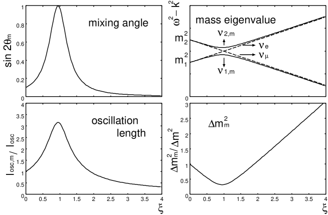
When $\xi=\cos{2\theta}$, the mixing angle in matter, $\theta_{\rm m}$, becomes maximum ($\pi/4$). This is called resonance and the resonance condition can be rewritten as

$$\rho_{\rm res}=1.3\times 10^{2}{\rm g}~{}{\rm cm}^{-3}\cos{2\theta}\left(\frac{0.5}{Y_{e}}\right)\left(\frac{1{\rm MeV}}{E}\right)\left(\frac{\Delta m^{2}}{10^{-5}{\rm eV}^{2}}\right).$$ (82)

At the resonance density, the matter oscillation length and the mass-squared difference become maximum and minimum, respectively:

$$(l_{\rm osc,m})_{\rm res}=\frac{l_{\rm osc}}{\sin{2\theta}},~{}~{}~{}~{}(\Delta m^{2}_{\rm m})_{\rm res}=\Delta m^{2}\sin{2\theta}.$$ (83)

On the other hand, in the case of anti-neutrino, the signature of the matter effect is different so that there is no resonance. However, we will discuss possible resonance in anti-neutrino sector later.

3.3.2 varying density

The solar neutrinos are produced at the center with the density about $150{\rm g}~{}{\rm cm}^{-3}$, and escape outward into vacuum. In this case and many more cases in astrophysical systems including supernovae, the neutrinos propagates in an inhomogeneous medium and the neutrino oscillation becomes much more complicated. As we saw in section 3.3.1, flavor eigenstates and mass eigenstates can be related by the effective mixing angles in matter as

$$\left(\begin{array}[]{c}\nu_{e}\\ \nu_{\mu}\\ \nu_{\tau}\end{array}\right)=U(\theta_{i,{\rm m}})\left(\begin{array}[]{c}\nu_{1,{\rm m}}\\ \nu_{2,{\rm m}}\\ \nu_{3,{\rm m}}\end{array}\right).$$ (84)

In an inhomogeneous matter, the mixing angles $\theta_{i,{\rm m}}$ are functions of $z$. Due to this dependence of the mixing angles on $z$, the wave equations cannot be solved analytically in general.

To see this, consider a two-flavor case. The wave equations were given in (76):

$$i\frac{\partial}{\partial z}\left(\begin{array}[]{c}\nu_{e}\\ \nu_{\mu}\end{array}\right)=\frac{\Delta m_{m}^{2}}{4E}\left(\begin{array}[]{cc}-\cos{2\theta_{\rm m}}&\sin{2\theta_{\rm m}}\\ \sin{2\theta_{\rm m}}&\cos{2\theta_{\rm m}}\end{array}\right)\left(\begin{array}[]{c}\nu_{e}\\ \nu_{\mu}\end{array}\right).$$ (85)

If the mixing matrix $U$ is constant, we can diagonalize the equations by multiplying $U$ to the both sides of (85). However, if the mixing matrix $U$ depends on $z$, the derivative operator $\partial/\partial z$ and $U$ do not commute so that the l.h.s. does not result in a simple form, although the r.h.s. is diagonalized:

$$i\frac{\partial}{\partial z}\left(\begin{array}[]{c}\nu_{1,{\rm m}}\\ \nu_{2,{\rm m}}\end{array}\right)+iU\left(\frac{\partial}{\partial z}U^{{\dagger}}\right)\left(\begin{array}[]{c}\nu_{1,{\rm m}}\\ \nu_{2,{\rm m}}\end{array}\right)=\frac{1}{2\omega}\left(\begin{array}[]{cc}m^{2}_{1,{\rm m}}&0\\ 0&m^{2}_{2,{\rm m}}\end{array}\right)\left(\begin{array}[]{c}\nu_{1,{\rm m}}\\ \nu_{2,{\rm m}}\end{array}\right).$$ (86)

Thus the equations are not effectively diagonalized and can be written as,

$$i\frac{\partial}{\partial z}\left(\begin{array}[]{c}\nu_{1,{\rm m}}\\ \nu_{2,{\rm m}}\end{array}\right)=\left(\begin{array}[]{cc}-\frac{\Delta m^{2}_{\rm m}}{2\omega}&-i\frac{\partial\theta_{\rm m}}{\partial z}\\ i\frac{\partial\theta_{\rm m}}{\partial z}&\frac{\Delta m^{2}_{\rm m}}{2\omega}\end{array}\right)\left(\begin{array}[]{c}\nu_{1,{\rm m}}\\ \nu_{2,{\rm m}}\end{array}\right).$$ (87)

This shows that even the mass eigenstates are mixing if the density is inhomogeneous and the magnitude of the mixing depends on $\partial\theta_{\rm m}/\partial z$.

Let us first consider the mixing of the mass eigenstates qualitatively. If the diagonal component is much larger than the off-diagonal component everywhere, that is,

$$\left|\frac{\partial\theta_{\rm m}}{\partial z}\right|\ll\frac{\Delta m^{2}_{\rm m}}{2\omega},$$ (88)

the mass eigenstates will propagate without mixing. In other words, the heavier state remains heavier and the lighter state remains lighter. There is no energy jump and this case can be said to be ”adiabatic”. Contrastingly, if the condition (88) is not satisfied, the heavier state can change to the lighter state and vice versa, which is a ”non-adiabatic” case. The non-adiabaticity is largest where the change of the mixing angle is rapid, which is expected to be around the resonance point as can be expected from Fig. 13.

Figure 14: Schematic view of two-flavor resonance in an inhomogeneous medium. The dashed lines show the masses of the mass eigenstates and the solid lines show the effective masses of the flavor eigenstates. Contribution from the neutral-current interactions are subtracted.

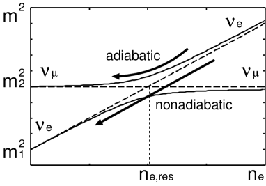
Fig. 14 will be helpful to understand the oscillation in an inhomogeneous matter. Assume that the vacuum mixing angle is so small that the lighter state is almost $\nu_{e}$, that is, $\nu_{e}$ is effectively ”ligher” than $\nu_{\mu}$ in vacuum. In a dense region, on the other hand, $\nu_{e}$ is effectively ”heavier” than $\nu_{\mu}$. The two flavors have the same ”mass” at the resonance point. Then let us consider a case where a $\nu_{e}$ is produced at a dense region and escape into vacuum as the solar neutrinos. If the resonance is adiabatic, the heavier state will remain heavier, which means that a $\nu_{e}$ produced at the dense region will emerge as a $\nu_{\mu}$. In contrast, if the resonance is non-adiabatic, a $\nu_{e}$ will remain a $\nu_{e}$.

Thus, the survival probability of $\nu_{e}$ depends largely on the adiabaticity of the resonance. The importance of the resonance in the solar neutrino problem was first pointed out by Mikheyev and Smirnov [226]. It was Bethe who found the essence of the MSW effect in an inhomogeneous medium to be the level crossing of the flavor eigenstates [34].

Let us discuss more quantitatively. The adiabatic condition (88) at the resonance point can be rewritten as,

$$1\ll\frac{\Delta m^{2}}{E\left|\frac{\partial\ln{n_{e}}}{\partial z}\right|_{\rm res}}\sin{2\theta}\tan{2\theta}.$$ (89)

The adiabaticity parameter $\gamma$ is defined as

$$\gamma\equiv\frac{\Delta m^{2}}{E\left|\frac{\partial\ln{n_{e}}}{\partial z}\right|_{\rm res}}\sin{2\theta}\tan{2\theta},$$ (90)

so that the adiabaticity condition is,

$$\gamma\gg 1.$$ (91)

What we want to know is the conversion probability of the matter eigenstates, $P_{\nu_{1,{\rm m}}\rightarrow\nu_{2,{\rm m}}}$. For a general profile of matter density, this cannot be obtained analytically. But for some special cases, analytic expression is known [182]. If we write the probability as,

$$P_{\nu_{1,{\rm m}}\rightarrow\nu_{2,{\rm m}}}=\frac{\exp{[-\frac{\pi\gamma F}{2}]}-\exp{[-\frac{\pi\gamma F}{2\sin^{2}{\theta}}]}}{1-\exp{[-\frac{\pi\gamma F}{2\sin^{2}{\theta}}]}},$$ (92)

the factor $F$ is given by,

$$F=\left\{\begin{array}[]{ll}1&(n_{e}\propto z)\\ \frac{(1-\tan^{2}{\theta})^{2}}{(1+\tan^{2}{\theta})^{2}}&(n_{e}\propto z^{-1})\\ 1-\tan^{2}{\theta}&(n_{e}\propto e^{-z/z_{0}})\end{array}\right..$$ (93)

Note that $P_{\nu_{1,{\rm m}}\rightarrow\nu_{2,{\rm m}}}\sim 1$ when $\gamma\gg 1$ and $P_{\nu_{1,{\rm m}}\rightarrow\nu_{2,{\rm m}}}\sim 0$ when $\gamma\ll 1$ in any cases, as expected.

If we obtain the conversion probability $P_{\nu_{1,{\rm m}}\rightarrow\nu_{2,{\rm m}}}$ in some way, we can compute, for example, the survival probability of $\nu_{e}$, $P_{\nu_{e}\rightarrow\nu_{e}}$. When a $\nu_{e}$ is produced at the center of the sun, the probabilities that it is $\nu_{1,{\rm m}}$ and $\nu_{2,{\rm m}}$ are $\cos^{2}{\theta_{\rm c}}$ and $\sin^{2}{\theta_{\rm c}}$, respectively, where $\theta_{\rm c}$ is the mixing angle at the center. First, if there is no conversion between $\nu_{1,{\rm m}}$ and $\nu_{2,{\rm m}}$, that is, if $P_{\nu_{1,{\rm m}}\rightarrow\nu_{2,{\rm m}}}=0$,

$$P_{\nu_{e}\rightarrow\nu_{e}} = \cos^{2}{\theta_{\rm c}}\cos^{2}{\theta}+\sin^{2}{\theta_{\rm c}}\sin^{2}{\theta}$$ (94)

$$= \frac{1+\cos{2\theta_{\rm c}}\cos{2\theta}}{2}.$$

On the other hand, when $P_{\nu_{1,{\rm m}}\rightarrow\nu_{2,{\rm m}}}$ is non-zero,

$$P_{\nu_{e}\rightarrow\nu_{e}} = \biggl{[}(1-P)\cos^{2}{\theta_{\rm c}}+P\sin^{2}{\theta_{\rm c}}\biggr{]}\cos^{2}{\theta}+\biggl{[}P\cos^{2}{\theta_{\rm c}}+(1-P)\sin^{2}{\theta_{\rm c}}\biggr{]}\sin^{2}{\theta}$$ (95)

$$= \frac{1+\cos{2\theta_{\rm c}}\cos{2\theta}}{2}-P\cos{2\theta_{\rm c}}\cos{2\theta},$$

where $P\equiv P_{\nu_{1,{\rm m}}\rightarrow\nu_{2,{\rm m}}}$.

In most cases, the survival probability is determined by the adiabaticity parameter $\gamma$. Because $\gamma$ depends on the neutrino parameters, mixing angles and mass differences, and density profile of matter, neutrino observation from various systems will allow us to investigate them.

If the matter density is much larger than the solar case, the two-flavor analysis is invalid and we have to take three flavors into account. This is exactly what we do later to consider neutrino oscillation in supernova. For a three flavor case, there are two resonance points. Although the situation will become more complicated, the essence is the same as the two-flavor case, the adiabaticity of the resonance.

3.4 Experiment of Neutrino Oscillation

Because the neutrino oscillation is a phenomenon beyond the standard model of particle physics, many experiments have been conducted to verify it in various systems. One of the attractive features of neutrino oscillation experiment is that it does not need high-energy accelerator.

In this section, we review neutrino oscillation experiments starting from general remarks about the experiments.

3.4.1 general remarks

The basic of neutrino oscillation experiment is to observe neutrinos from a known source. Although all flavors except sterile neutrino can be ideally detected, $\nu_{e}$ and $\bar{\nu}_{e}$ are easier to detect than other flavors so that they are often used as signal. In this respect, neutrino oscillation experiment can be classified into two types. One is called ”appearance experiment”, in which, for example, we detect neutrinos from a $\nu_{\mu}$ source. If we observe even a single event of $\nu_{e}$, this is an evidence of flavor conversion. Another type is called ”disappearance experiment”, in which we observe $\nu_{e}$s ($\bar{\nu}_{e}$s) from a $\nu_{e}$ ($\bar{\nu}_{e}$) source with known flux. If we observe less number of $\nu_{e}$s, this can also be an evidence of flavor conversion.

Each type has its own advantage and disadvantage. By the appearance experiment, we cannot reject neutrino oscillation phenomenon even if we did not observe the signal. This is because $\nu_{\mu}$ might have changed into $\nu_{\tau}$, not $\nu_{e}$. Contrastingly, the disappearance experiment can tell whether neutrino oscillation occurred or not, if only $\nu_{e}$s were converted into any type of neutrino. However, we cannot know the oscillation channel, that is, which flavor $\nu_{e}$s were converted to. In this respect, the appearance experiment can probe a selected channel of neutrino oscillation.

Many kinds of experiments have been done so far and each has different parameter region it can probe. Here we discuss how the neutrino parameters can be probed. More concretely, let us consider what we could know if there was no signal in an appearance experiment. For simplicity, we consider just two-flavor oscillation in vacuum. As we saw in section 3.2, conversion probability $P_{\nu_{\mu}\rightarrow\nu_{e}}$ as a function of the propagation distance is,

$$P_{\nu_{\mu}\rightarrow\nu_{e}}(z)=\sin^{2}{2\theta}\sin^{2}\left(\frac{\pi z}{l_{\rm osc}}\right)$$ (96)

If we detect no $\nu_{e}$ signal, it means that the conversion probability is smaller than a certain value $\delta$ which is determined by the noise level of the experiment. When the baseline $L$ is much smaller than the oscillation length $\ell_{\rm osc}$, it is written as,

$$P_{\nu_{\mu}\rightarrow\nu_{e}}(L)\approx\sin^{2}{2\theta}\left(\frac{\pi L}{l_{\rm osc}}\right)^{2}<\delta.$$ (97)

Substituting the definition of $\ell_{\rm osc}$ (50), this reduces to

$$\Delta m^{2}\sin{2\theta}<\frac{E\sqrt{\delta}}{L}.$$ (98)

On the other hand, when $L\gg\ell_{\rm osc}$, finite energy width of the neutrino beam will average the oscillation of the conversion probability so that the no signal means,

$$P_{\nu_{\mu}\rightarrow\nu_{e}}(L)=\frac{1}{2}\sin^{2}{2\theta}<\delta,$$ (99)

which reduces to,

$$\sin{2\theta}<\sqrt{2\delta}.$$ (100)

Note that we cannot obtain information about $\Delta m^{2}$ in this case.

Thus if we want to probe small $\Delta m^{2}$, experiments with small $E/L$ are advantageous. Various systems with characteristic neutrino energy, baseline and possible $\Delta m^{2}$ which can be probed are shown in Table 2. Analysis of an disappearance experiment can be done essentially in the same way.

Table 2: Probe of squared mass difference by various experiments.

source	energy $E({\rm MeV})$	baseline $L({\rm m})$	$\Delta m^{2}({\rm eV}^{2})$
accelerator	$10^{3}\sim 10^{5}$	$10^{2}\sim 10^{6}$	$10^{-3}\sim 10^{2}$
reactor	$1\sim 2$	$10\sim 10^{5}$	$10^{-5}\sim 10^{-1}$
atmosphere	$\sim 10^{3}$	$10^{5}\sim 10^{7}$	$10^{-2}\sim 10^{-4}$
Sun	$\sim 1$	$\sim 10^{11}$	$\sim 10^{-11}$

3.4.2 accelerator experiment

Accelerator experiment is the most popular experiment of neutrino oscillation. One of the advantage of accelerator experiment is that we can control the neutrino source while Sun, atmosphere and supernovae are uncontrolled and rather unknown sources. Although there have been a lot of accelerator experiments so far, the basic concept is similar as we will review below.

First, protons are accelerated and collided with target nuclei to produce $\pi^{\pm}$:

$$p+N\rightarrow\pi^{+}\;,\;\pi^{-},\cdots.$$ (101)

Then $\pi^{+}$s or $\pi^{-}$s are absorbed and the others decay to produce neutrinos. For example,

$$\pi^{+}\rightarrow\mu^{+}+\nu_{\mu},$$ (102)

$$\mu^{+}\rightarrow e^{+}+\nu_{e}+\bar{\nu}_{\mu}$$ (103)

In this way, if $\pi^{-}$s are absorbed completely, we have a neutrino beam which consists of $\nu_{e}$, $\nu_{\mu}$ and $\bar{\nu}_{\mu}$. Thus, if we detect $\bar{\nu}_{e}$s in this beam, we can confirm neutrino oscillation $\bar{\nu}_{\mu}\rightarrow\bar{\nu}_{e}$. In fact, $\pi^{-}$s can not be absorbed completely and decay like,

$$\pi^{-}\rightarrow\mu^{-}+\bar{\nu}_{\mu},$$ (104)

$$\mu^{-}\rightarrow e^{-}+\bar{\nu}_{e}+\nu_{\mu}.$$ (105)

Consequently, some $\bar{\nu}_{e}$s will be produced and they become one of main noises in this kind of experiment.

Table 3: Accelerator experiments

experiment	baseline	neutrino energy	detector	status	reference
CCFR	$\sim 1{\rm km}$	$30-500{\rm GeV}$	690 ton target calorimeter	completed	[63, 64]
NuTeV	$1.4{\rm km}$	$\sim 100{\rm GeV}$	690 ton target calorimeter	completed	[63, 255]
KARMEN	$17.5{\rm m}$	$\sim 50{\rm MeV}$	$56{\rm ton}$ liquid scintillator	completed	[167, 168]
LSND	$30{\rm m}$	$\sim 50{\rm MeV}$	$167{\rm ton}$ liquid scintillator	completed	[207, 208, 209]
NOMAD	$625{\rm m}$	$\sim 50{\rm GeV}$	2.7 ton drift chambers	completed	[253, 254]
MiniBooNE	$490{\rm m}$	$0.1\sim 2{\rm GeV}$	$445{\rm ton}$ mineral oil	ongoing	[230, 231]
K2K	$250{\rm km}$	$\sim 1{\rm GeV}$	$22500{\rm ton}$ water (SK)	ongoing	[158, 159, 160]
					and [161]

Figure 15: Parameter regions allowed by the LSND observation (purple, blue). Exclusion curves from various other experiments are shown as well, with the region on the right side excluded [254].

Figure 16: Expected excluded regions in case of a non-observation of signal in MiniBooNE [231].

Figure 17: The reconstructed energy spectrum for the $\nu_{\mu}$-like sample. Points with error bars are data. The solid line is the best fit spectrum and the dashed line is the expected spectrum without oscillation [161].

Figure 18: Allowed regions of oscillation parameters for $\nu_{\mu}\rightarrow\nu_{\tau}$. Dashed, solid and dot-dashed lines are 68.4 %, 90 % and 99 % C.L. contours, respectively [161].

In this experiment, we can control the amount of the produced neutrinos. If there are $\bar{\nu}_{e}$ events we can compute the conversion probability $P_{\bar{\nu}_{\mu}\rightarrow\bar{\nu}_{e}}$. Or, we can obtain an upper limit for the conversion probability if no signal was obtained. Anyway, we can extract information about neutrino parameters as we saw in section 3.4.1.

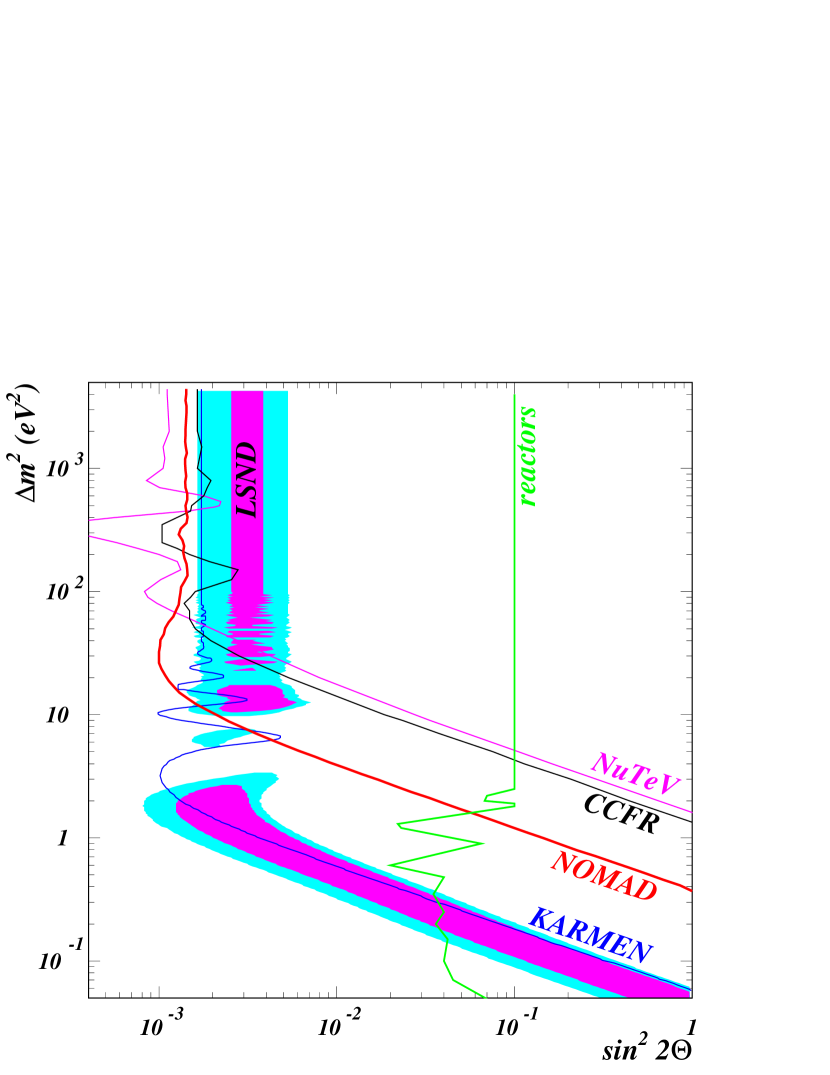
The current and past accelerator experiments are classified into long-baseline experiments and short-baseline experiments. Of course, the latter is technically easier so that early experiments have rather short baselines. However, implication from the recent solar and atmospheric neutrino observations has made it necessary to probe very small $\Delta m^{2}$ by long-baseline experiments. Features of some of the current and past accelerators are shown in Table 3. Among them, CCFR, NuTeV, KARMEN and NOMAD had no signal for neutrino oscillation and obtained constraints on oscillation parameters which are shown in Fig. 16.

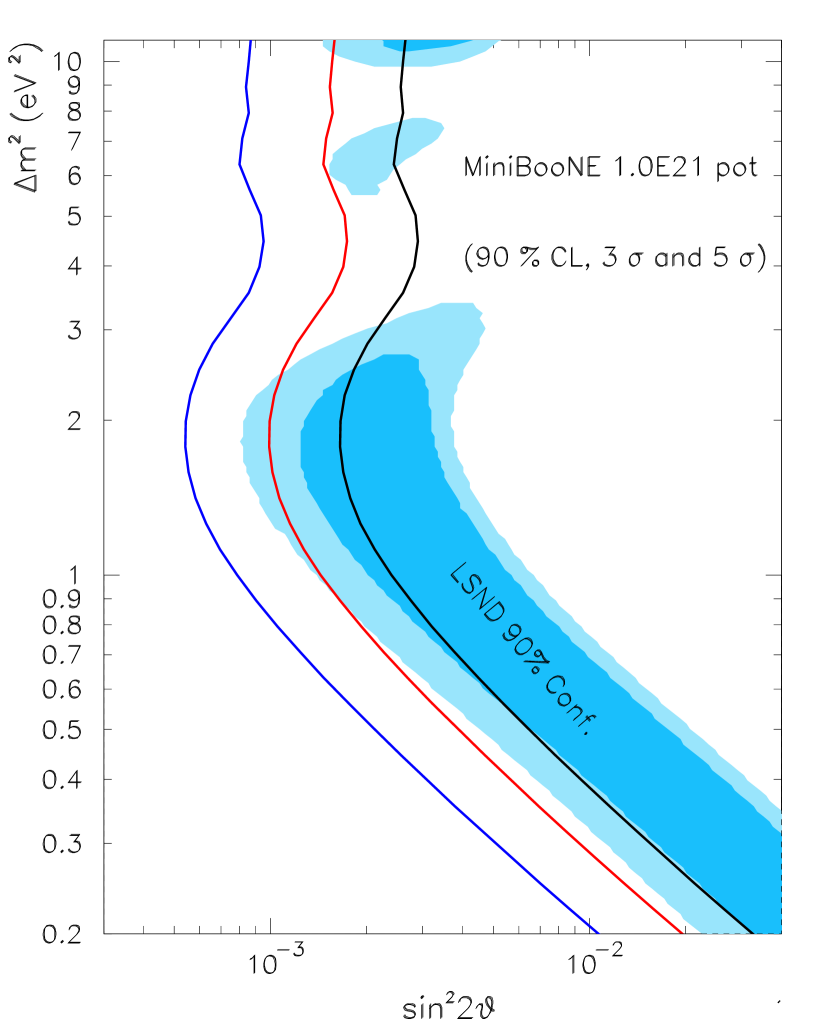
The LSND experiment performed at Los Alamos observed $87.9\pm 22.4\pm 6.0$ excess events in the $\bar{\nu}_{\mu}\rightarrow\bar{\nu}_{e}$ appearance channel [209]. This signal corresponds to a transition probability of $P=(0.264\pm 0.067\pm 0.045)\%$, which is $\sim 3.3\sigma$ away from zero. If we interpret it in terms of two-flavor oscillation, parameter regions shown in Fig. 16 are allowed. Although most of the allowed regions are excluded by other experiments, there are still some surviving regions with $\Delta m_{\rm LSND}^{2}\approx 0.1-1{\rm eV}^{2}$. This remaining regions are expected to be confirmed or denied by the MiniBooNE experiment [230, 231] in the near future. Fig. 16 shows expected excluded regions in case of a non-observation of signal in MiniBooNE.

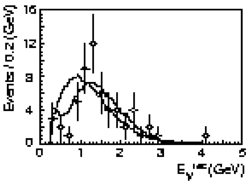
The K2K experiment [158, 159, 160, 161], the KEK to Kamioka long-baseline neutrino oscillation experiment, is an accelerator based project with 250 km baseline which is much longer than those of the past experiments. This long baseline make it possible to explore neutrino oscillation in the same $\Delta m^{2}$ region as atmospheric neutrinos. In [161], five-year data with 57 $\nu_{\mu}$ candidates was reported and their energy distribution is shown in Fig. 18. The distortion of energy spectrum, which signals neutrino oscillation, is clearly seen in Fig. 18 and the probability that the result would be observed without neutrino oscillation is $0.0050\%(4.0\sigma)$. Fig. 18 shows a two-flavor neutrino oscillation analysis with $\nu_{\mu}$ disappearance. The best fit point is,

$$\sin^{2}{2\theta}=1.0,~{}~{}~{}\Delta m^{2}=2.8\times 10^{-3}{\rm eV}^{2}.$$ (106)

3.4.3 reactor experiment

Table 4: Reactor experiments

experiment	baseline	status	reference
Bugey (France)	$15,40,95{\rm m}$	completed	[1]
CHOOZ (France)	$1{\rm km}$	completed	[67, 68]
Palo Verde (USA)	$750{\rm m}$	completed	[39, 40]
KamLAND (Japan)	$100{\rm km}\sim$	running	[164, 165, 166]

In nuclear reactors, $\bar{\nu}_{e}$s are isotropically emitted by $\beta$-decay of neutron-rich nuclei. Reactor experiment of neutrino oscillation is detecting these $\bar{\nu}_{e}$s and seeing if there is a deficit compared with the expected flux. The flux and spectrum of $\bar{\nu}_{e}$ are determined by the power of the reactor and abundance of ²³⁵U, ²³⁸U, ²³⁹Pu and ²⁴¹Pu. Because reactor neutrinos have relatively low energy, they are well suited in exploring the region of small $\Delta m^{2}$ at modest baselines. For example, to explore the parameter $\Delta m^{2}$ down to $10^{-3}{\rm eV}^{2}$ a reactor experiment with energy around 5 MeV requires a baseline of $L=1$ km, while an accelerator experiment with $E=5$ GeV would require $L=1,000$ km.

Figure 19: Constraint to conversion $\bar{\nu}_{e}\rightarrow\bar{\nu}_{x}$ from CHOOZ experiment [68] and that of conversion $\bar{\nu}_{\mu}\rightarrow\bar{\nu}_{e}$ from K2K experiment [160].

Figure 20: Prompt event energy spectrum of $\bar{\nu}_{e}$ candidate events with associated background spectra. The shaded band indicates the systematic error in the best-fit reactor spectrum above 2.6 MeV [166].

Figure 21: (a) Neutrino oscillation parameter allowed region from KamLAND anti-neutrino data (shaded regions) and solar neutrino experiments (lines) which we discuss later [166]. (b) Result of a combined two-neutrino oscillation analysis of KamLAND and the observed solar neutrino fluxes.

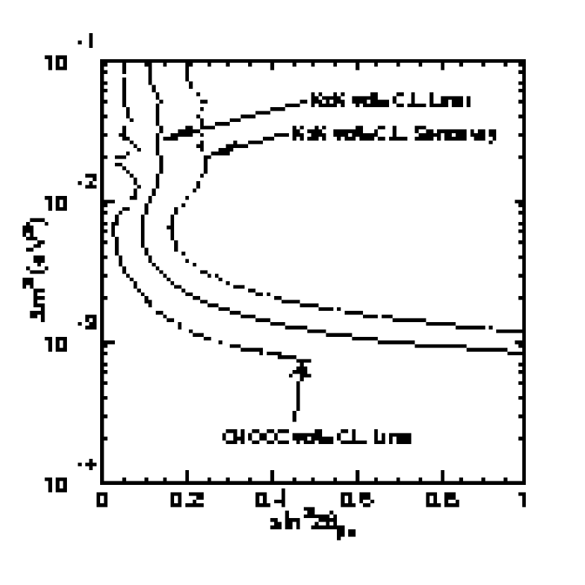
The current and past reactor experiments are shown in Table 4. Among these, CHOOZ [68] gives the strongest constraint on the mixing angle of $\bar{\nu}_{e}\rightarrow\bar{\nu}_{x}$ for $\Delta m^{2}>10^{-3}{\rm eV}^{2}$ (Fig. 21).

Inspired by the recent development of solar neutrino observation, a long-base line experiment called KamLAND [164, 165, 166] was constructed where there was once the Kamiokande detector. KamLAND consists of 1000ton liquid scintillator and its primary purpose is to confirm the solution to the solar neutrino problem, which will be discussed later. There are 16 reactors with distances about 100 $\sim$ 1000km from KamLAND so that the $\bar{\nu}_{e}$ flux at KamLAND is sufficiently large to probe neutrino oscillation Because of the long baseline and detectability of low-energy neutrinos, KamLAND can probe much smaller $\Delta m^{2}$ compared with the past experiments.

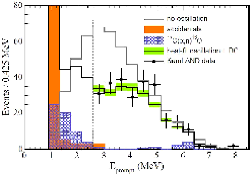
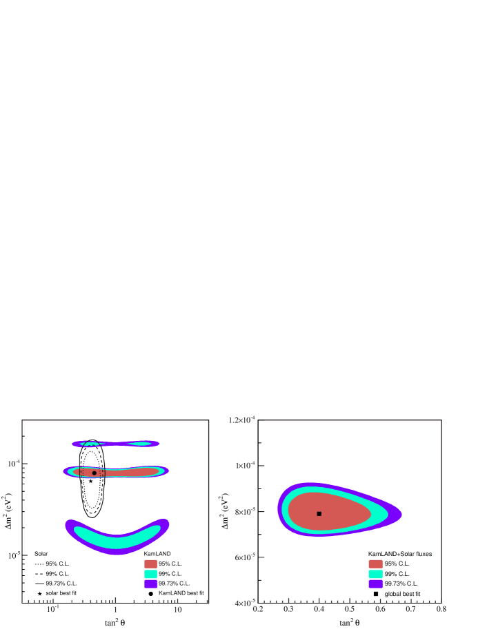
Fig. 21 shows the prompt event energy spectrum of $\bar{\nu}_{e}$ candidate events with associated background spectra [166]. They observed 258 $\bar{\nu}_{e}$ candidate events with energies above 3.4 MeV compared to 365.2 events expected in the absence of neutrino oscillation. Accounting for 17.8 expected background events, the statistical significance for reactor $\bar{\nu}_{e}$ disappearance is 99.998%. Also the observed energy spectrum disagrees with the expected spectral shape in the absence of neutrino oscillation at 99.6% significance and prefers the distortion expected from $\bar{\nu}_{e}$ oscillation effects rather than those from neutrino decay and decoherence. A two-neutrino oscillation analysis of the KamLAND data gives

$$\Delta m^{2}=7.9^{+0.6}_{-0.5}\times 10^{-5}{\rm eV}^{2},$$ (107)

as shown in Fig. 21. A global analysis of data from KamLAND and solar neutrino experiments, which will be discussed later, yields

$$\Delta m^{2}=7.9^{+0.6}_{-0.5}\times 10^{-5}{\rm eV}^{2},\tan^{2}{\theta}=0.40^{+0.10}_{-0.07}.$$ (108)

3.4.4 atmospheric neutrino

Figure 22: The zenith angle distribution for fully-contained 1-ring events [315]. The points show the data, box histograms show the non-oscillated Monte Carlo events and the lines show the best-fit expectations for $\nu_{\mu}\leftrightarrow\nu_{\tau}$ oscillations with $\sin^{2}{2\theta}=1.00$ and $\Delta m^{2}=2.1\times 10^{-3}{\rm eV}^{2}$. The height of the boxes shows the statistical error of the Monte Carlo.

When cosmic rays enter the atmosphere, they collide with the atmospheric nuclei to produce a lot of mesons (mostly pions):

$$N_{\rm CR}+N_{\rm air}\rightarrow\pi^{\pm},\pi^{0},\cdots.$$ (109)

The pions decay and the decay product, such muons, further decay to produce neutrinos:

$$\pi^{\pm}\rightarrow\mu^{\pm}+\nu_{\mu}(\bar{\nu}_{\mu}),~{}~{}~{}\mu^{\pm}\rightarrow e^{\pm}+\nu_{e}(\bar{\nu}_{e})+\bar{\nu}_{\mu}(\nu_{\mu})$$ (110)

When cosmic rays enter the atmosphere, they collide with the atmospheric nuclei to produce a lot of mesons (mostly pions):

$$N_{\rm CR}+N_{\rm air}\rightarrow\pi^{\pm},\pi^{0},\cdots.$$ (111)

The pions decay and the decay product, such as muons, further decay to produce neutrinos:

$$\pi^{\pm}\rightarrow\mu^{\pm}+\nu_{\mu}(\bar{\nu}_{\mu}),~{}~{}~{}\mu^{\pm}\rightarrow e^{\pm}+\nu_{e}(\bar{\nu}_{e})+\bar{\nu}_{\mu}(\nu_{\mu})$$ (112)

These neutrinos are called the atmospheric neutrinos and they provided the first strong indication for neutrino oscillation. Their energy range and path length varies from 0.1 to 10 GeV and from 10 to 10,000 km, respectively, which indicates that atmospheric neutrinos can provide an opportunity for oscillation studies over a wide range of energies and distances. From (112), we simply expect that the flux ratio $(\nu_{\mu}+\bar{\nu}_{\mu})/(\nu_{e}+\bar{\nu}_{e})=2$. This is roughly correct, even though the ratio depends on a lot of factors such as neutrino energy and zenith angle of the incoming neutrino if detailed decay processes and geometric effects are taken into account [29, 139, 140]. However, the results from many experiments showed that this ratio was about unity. This was once called the atmospheric neutrino problem, which is now interpreted successfully in terms of neutrino oscillation. In fact, the SK was the first to prove neutrino oscillation phenomenon by its observation of the atmospheric neutrino with a high accuracy.

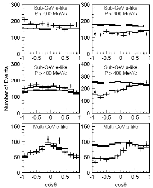
It was reliable identification of $\nu_{\mu}$ that allowed SK to prove neutrino oscillation. Because the SK detector is huge (diameter $\sim$ 39m and height $\sim$ 42m), $\nu_{\mu}$s with energy $\sim 1$ GeV can be identified as fully contained events, for which all neutrino-induced interactions occur in the detector and neutrino energies and directions can be accurately obtained. The results from SK are shown in Fig. 22. As can be seen, $\nu_{e}$ flux is consistent with the theoretical calculation while there is a deficit in $\nu_{\mu}$ flux. It indicates that $\nu_{\mu}\leftrightarrow\nu_{\tau}$ oscillation would be solution to the atmospheric neutrino problem. In Fig. 23, allowed oscillation parameters for $\nu_{\mu}\leftrightarrow\nu_{\tau}$ oscillations are shown. The best fit values are

$$\Delta m^{2}_{\rm atm}=2.1\times 10^{-3}{\rm eV}^{2},~{}~{}~{}\sin^{2}{\theta_{\rm atm}}=1.00.$$ (113)

These results are confirmed by other experiments such as Soudan 2 [316] and MACRO [214, 215] (see also [109]).

Figure 23: Allowed oscillation parameters for $\nu_{\mu}\leftrightarrow\nu_{\tau}$ oscillations from the atmospheric neutrino observation at SK [315]. Three contours correspond to the 68% (dotted line), 90% (solid line) and 99% (dashed line) C.L. allowed regions.

As we saw in Eq. (49), the conversion and survival probabilities depends on $L/E$, where $L$ and $E$ are neutrino path length and energy, and oscillates with respect to $L/E$. This behavior was confirmed by the atmospheric neutrino observation at SK [313]. This means that it rejected other possibilities such as neutrino decay and decoherence which had different dependence on $L/E$ and proved that solution to the atmospheric neutrino problem was truly neutrino oscillation.

3.4.5 solar neutrino

In the central region of the sun, $\nu_{e}$s are continuously produced by the hydrogen fusion,

$$4p\rightarrow{}^{4}{\rm He}+2e^{+}+2\nu_{e}+26.731{\rm MeV}.$$ (114)

These neutrinos are called solar neutrinos. The first experiment of the solar neutrino observation was the chlorine experiment at Homestake by R. Davis and his collaborators in the 1960’s [74, 71]. On the other hand, the theoretical study of the solar neutrino was pioneered by J. N. Bahcall. The neutrino production rate in the sun has been calculated based on the standard solar model, which reproduces the current state of the sun by following the evolution of a main-sequence star with solar metalicity and mass. The solar neutrino flux calculated by the current standard solar model [22, 24] is shown in Fig. 25.

Figure 24: Solar neutrino flux from various nuclear reactions [24].

Figure 25: Observed and predicted fluxes of solar neutrino [19].

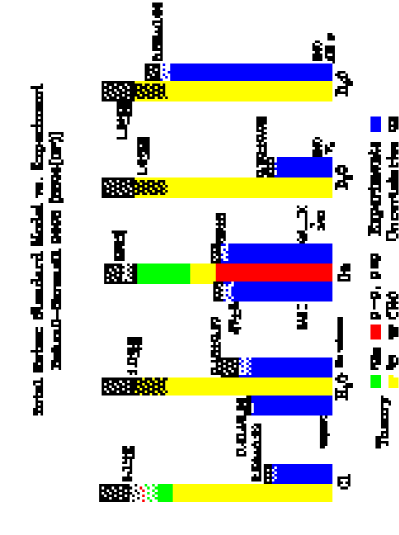
However, the fluxes observed by several detectors have been substantially smaller than the predicted flux (Fig. 25). This is so called solar neutrino problem and has been studied for several decades (for reviews, see [114, 21], and a text book by Bahcall [20]). Historically, the solar neutrino problem was attributed to incompleteness of the solar model and/or unknown neutrino property including neutrino oscillation. With the improvement of both the solar model and observation, especially at SuperKamiokande [307, 310, 311, 314], it is now common to think that the uncertainties of the solar model cannot solely explain the gap between the observations and prediction.

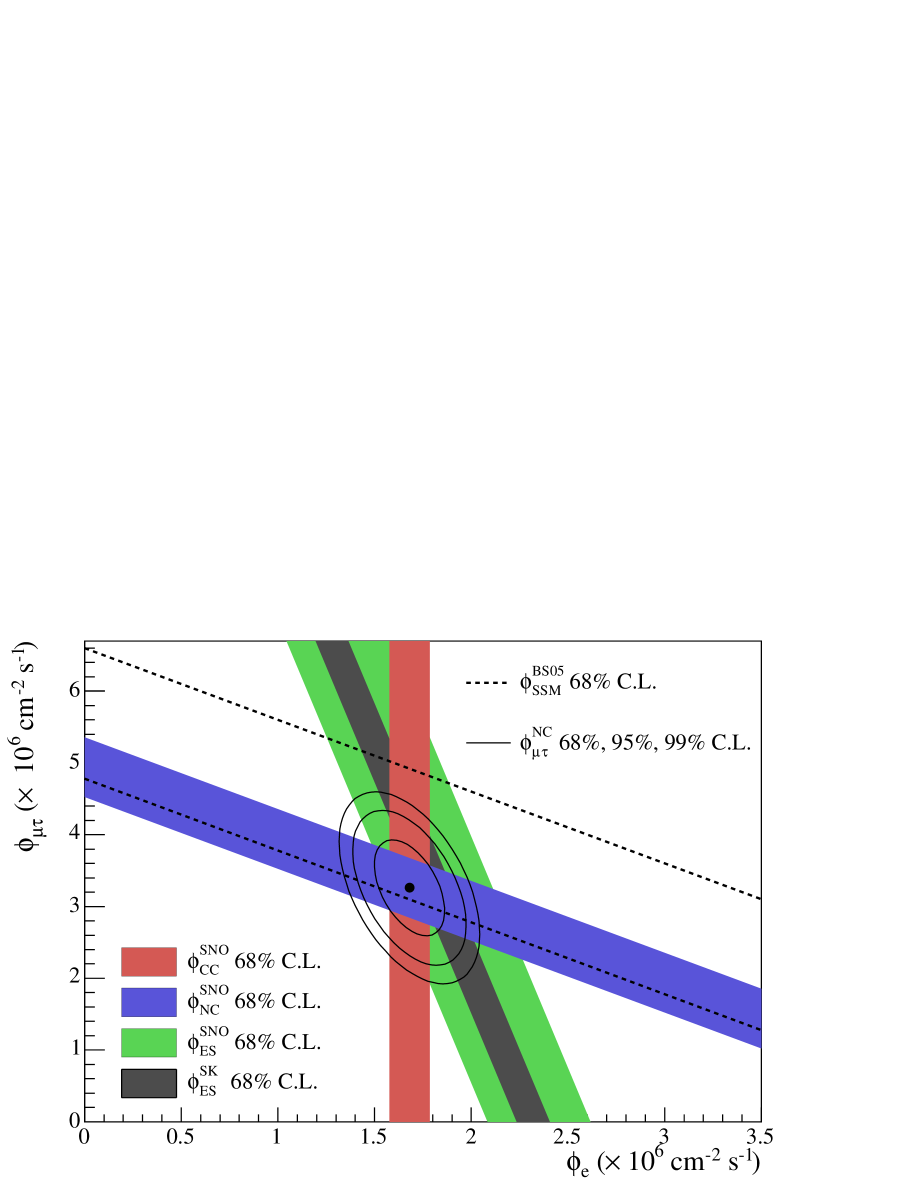
The critical observation has been conducted by Sudbury Neutrino Observatory (SNO) [295, 296, 297, 298], which clearly showed that electron neutrinos are converted to the other flavors. The SNO was designed primarily to search for a clear indication of neutrino flavor conversion for solar neutrinos without relying on solar model calculations. Its significant feature is the use of 1000 tons of heavy water which allows the distinction between the following three signal:

$$\nu_{e}+d\rightarrow p+p+e^{-},$$ (115)

$$\nu+d\rightarrow p+n+\nu,$$ (116)

$$\nu+e^{-}\rightarrow\nu+e^{-}.$$ (117)

Here the reaction (115) occurs through the charged current interaction and is relevant only to $\nu_{e}$, while the other two reactions are through the neutral current interaction and sensitive to all flavors. It should be noted that SK can identify only the electron scattering event (117) for energies of the solar neutrinos ($<10{\rm MeV}$), although its volume is much larger than that of SNO.

Fig. 27 shows the fluxes of $\mu+\tau$ neutrinos and electron neutrinos obtained from SNO [298] and SK [312]. Combining the signals from the three channels, it clearly shows that there is non-zero flux of $\nu_{\mu}$ and $\nu_{\tau}$, which is a strong evidence of neutrino flavor conversion. If we interpret these data by 2-flavor neutrino oscillation $\nu_{e}\leftrightarrow\nu_{x}$, we obtain constraint on the mixing angle and mass-squared difference as in Fig. 27 with the best fit:

$$\Delta m^{2}_{\rm solar}=6.5^{+4.4}_{-2.3}\times 10^{-5}{\rm eV}^{2},~{}~{}~{}\tan^{2}{\theta_{\rm solar}}=0.45^{+0.09}_{-0.08}.$$ (118)

Also it should be noted that, as can be seen in Fig. 27, the prediction of the standard solar model is, at least concerning the high-energy neutrinos, confirmed by the observation.

Figure 26: Flux of $\mu+\tau$ neutrinos versus flux of electron neutrinos obtained from SNO [298] and SK [312]. The total ⁸Be solar neutrino flux predicted by the Standard Solar Model [24] is shown as dashed lines. The point represents $\phi_{e}$ from the CC flux and $\phi_{\mu\tau}$ from the NC-CC difference with 68%, 95%, and 99% C.L. contours included.

Figure 27: Global neutrino oscillation analysis using solar neutrino data [298]. The solar neutrino data includes SNO data, the rate measurements from the Cl, SAGE, Gallex/GNO, and SK-I zenith spectra.

3.4.6 current status of neutrino parameters

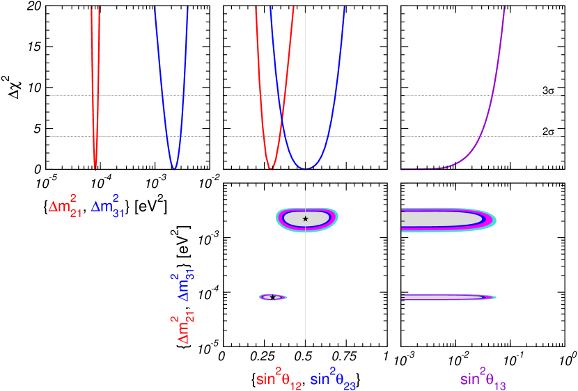
Here we summarize the information of neutrino oscillation parameters obtained so far. Combined analysis based on all the data from various neutrino oscillation experiments has been done by many authors [92, 113, 217, 218, 300]. Basically three-flavor neutrino oscillation can explain all the data reasonably except the LSND data discussed in section 3.4.2. Maltoni et al. [218] performed a general fit to the global data in the five-dimensional parameter space ($\theta_{12},\theta_{23},\theta_{13},\Delta m_{12}^{2}$ and $\Delta m_{13}^{2}$), and showed projections onto various one- or two-dimensional subspaces. They gave,

• $\sin^{2}{\theta_{12}}\approx 0.30$, mostly from solar neutrino data

• $\sin^{2}{\theta_{23}}\approx 0.50$, mostly from atmospheric neutrino data

• $\sin^{2}{\theta_{13}}\leq 0.30$, mostly from atmospheric neutrino and CHOOZ data

• $\Delta m_{12}^{2}\approx 8.1\times 10^{-5}{\rm eV}^{-2}$, mostly from KamLAND data

• $|\Delta m_{13}^{2}|\approx 2.2\times 10^{-3}{\rm eV}^{-2}$, mostly from atmospheric neutrino data

and allowed regions of the parameters are summarized in Table 5 and Fig. 29. We can see that most of the parameters are known with high accuracies.

Contrastingly, we have rather poor information on some of key neutrino parameters. First, only a loose upper bound has been obtained for $\sin^{2}{\theta_{13}}$. As we will discuss in section LABEL:section:nu-osc_SN, this parameter acts an important role in supernova neutrino oscillation.

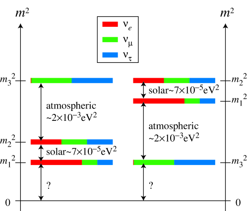
The next is the signature of $\Delta m_{13}^{2}$. There are two mass schemes according to the signature (Fig. 29). One is called normal hierarchy with $m_{1}^{2}\approx m_{2}^{2}\ll m_{3}^{2}$ and another is called inverted hierarchy with $m_{3}^{2}\ll m_{1}^{2}\approx m_{2}^{2}$. The mass scheme is also crucial when we consider neutrino oscillation in supernova.

The value of CP violation parameter (see Eq. (42)) is not known either. Although it would have small impact on supernova neutrino oscillation so that we have neglected it, it is important in considering the structure and origin of neutrino masses. Also it will be important particle-theoretically whether $\theta_{23}$ is maximal ($\pi/4$) or not and whether $\theta_{13}$ is exactly zero or just small.

As we saw in section 3.4.2, the LSND experiment gave us an implication of $\bar{\nu}_{\mu}\rightarrow\bar{\nu}_{e}$ oscillation with $\Delta m_{\rm LSND}^{2}\approx 1{\rm eV}^{2}$. However, noting that $\Delta m_{\rm LSND}^{2}\gg\Delta m_{\rm atm}^{2}\gg\Delta m_{\rm solar}^{2}$, it is easy to see that three-flavor oscillation scheme discussed above cannot explain the LSND data. This is because we have only two independent mass-squared differences with three flavors and they are completely determined by the solar, atmospheric, reactor and accelerator experiments. If the LSND results are confirmed by another experiment like MiniBooNE, we will need some new physics beyond the standard three-flavor neutrino oscillation. One possibility is to add an extra neutrino which mixes with standard neutrinos. It must not have a charge of weak interaction because the LEP experiments imply that there are no very light degrees of freedom which couple to Z-boson [196]. Thus the extra neutrino must be sterile. We will not discuss sterile neutrino further in this review. For further study about sterile neutrino, see [70, 299] and references therein.

Table 5: Best-fit values, 2$\sigma$, 3$\sigma$, and 4$\sigma$ intervals (1 d.o.f.) for the three-flavor neutrino oscillation parameters from global data [218].

parameter	best fit	2$\sigma$	3$\sigma$	4$\sigma$
$\Delta m^{2}_{21}\>[10^{-5}{\rm eV}^{2}]$	8.1	7.5–8.7	7.2–9.1	7.0–9.4
$\Delta m^{2}_{31}\>[10^{-3}{\rm eV}^{2}]$	2.2	1.7–2.9	1.4–3.3	1.1–3.7
$\sin^{2}\theta_{12}$	0.30	0.25–0.34	0.23–0.38	0.21–0.41
$\sin^{2}\theta_{23}$	0.50	0.38–0.64	0.34–0.68	0.30–0.72
$\sin^{2}\theta_{13}$	0.000	$\leq$ 0.028	$\leq$ 0.047	$\leq$ 0.068

Figure 28: Projections of the allowed regions from the global oscillation data at 90%, 95%, 99%, and 3$\sigma$ C.L. for 2 d.o.f. for various parameter combinations. Also shown is $\Delta\chi^{2}$ as a function of the oscillation parameters $\sin^{2}{\theta_{12}},\sin^{2}{\theta_{23}},\sin^{2}{\theta_{13}},\Delta m^{2}_{21},\Delta m^{2}_{31}$, minimized with respect to all undisplayed parameters [218].

Figure 29: Possible configurations of neutrino mass states as suggested by oscillations: the normal (left) and inverted (right) hierarchy. The flavor composition is shown as well [89, 90].

4 Neutrino Oscillation in Supernova

4.1 Overview

As we saw in section 2, core-collapse supernovae are powerful sources of neutrinos with total energies about $10^{53}$ erg. Since neutrinos are considered to dominate the dynamics of supernova, they reflect the physical state of deep inside of the supernova, which cannot be seen by electromagnetic waves. Neutrinos are emitted by the core and pass through the mantle and envelope of the progenitor star. Since the interactions between matter and neutrinos are extremely weak, one may expect that neutrinos bring no information about the mantle and envelope. In fact, they do bring the information through neutrino oscillation because resonant oscillation discussed in section 3.3.2 depends on the density profile around the resonance point. Thus neutrinos are also a useful tool to probe the outer structure of supernova, including propagation of shock waves.

On the other hand, supernova has been attracting attention of particle physicist, too, because it has some striking features as a neutrino source. As we discussed in section 3.4, there have been a lot of neutrino oscillation experiment, which allowed us to know many important parameters such as mixing angles and mass-squared differences. However, there are still some unknown parameters and physical structure of neutrinos which are difficult to probe by the conventional approaches. In this situation, supernova has been expected to give us information on fundamental properties of neutrinos which cannot be obtained from other sources.

4.2 Supernova Neutrino

Here we review the basic properties of neutrinos emitted during various phases from the onset of the gravitational collapse to the explosion. Supernova is roughly a blackbody source for neutrinos of all flavors with a temperature of several MeV. What is important, in the context of neutrino oscillation, is that each flavor has a different temperature, flux and its time evolution. The differences are significant especially among $\nu_{e}$, $\bar{\nu}_{e}$ and the other flavors denoted $\nu_{x}$. Although the quantitative understanding of the differences are not fully established in the current numerical simulation, we can still have qualitative predictions and some quantitative predictions.

4.2.1 neutrino emission during various phases

Here let us follow again the supernova processes discussed in section 2 focusing on neutrinos. First of all, the core collapse is induced by electron capture,

$$e^{-}+A\rightarrow\nu_{e}+A^{\prime},$$ (119)

which produces $\nu_{e}$s. They can escape freely from the core because the core is optically thin for the neutrinos in the early stage of the collapse. However, the luminosity is negligible compared with the later phases.

As the core density increases, the mean free path of $\nu_{e}$, $\lambda_{\nu}$, becomes smaller due to the coherent scattering with nuclei, $\nu_{e}A\rightarrow\nu_{e}$. Neutrinosphere is formed when the mean free path $\lambda_{\nu}$ becomes smaller than the core size, $R$. Further, if the diffusion timescale of $\nu_{e}$,

$$t_{\rm diff}\approx\frac{3R^{2}}{c\lambda_{\nu}},$$ (120)

is larger than the dynamical timescale of the core,

$$t_{\rm dyn}\approx\frac{1}{\sqrt{G\rho}},$$ (121)

$\nu_{e}$s cannot escape from the core during the collapse, that is, $\nu_{e}$s are trapped. When neutrinos are trapped and become degenerate, the average neutrino energy increases and the core become optically-thicker because the cross section of the coherent scattering increases as $\sigma_{\rm coh}\propto E_{\nu}^{2}$. Since low-energy neutrinos can escape easily from the core, most of neutrinos emitted during the collapse phase have relatively low energy ($<30{\rm MeV}$).

Figure 30: Time evolution of neutrino luminosities calculated by a numerical model of a $25M_{\odot}$ progenitor star with a $2.05M_{\odot}$ core [219]. The neutronization peak is drawn to be half the actual value. Here $\nu,\bar{\nu}$ and $\mu$ denote $\nu_{e},\bar{\nu}_{e}$ and $\nu_{x}$, respectively.

Figure 31: Electron neutrino luminosity and motion of mass shells based on the same model as the one in Fig. 31 [219]. The neutrino luminosities increase when outer core matter accretes onto the protoneutron star.

The collapse of the inner core stops when the central density exceeds the nucleus density and a shock wave stands between the inner core and the outer core falling with a super-sonic velocity. It should be noted that the shock wave stands in a region with a high density ($\approx 10^{12}\sim 10^{14}{\rm g/cc}$), which is much deeper than where the neutrinosphere is formed ($\approx 10^{10}\sim 10^{12}{\rm g/cc}$).

In the shocked region, nuclei are decomposed into free nucleons. Because the cross section of the coherent scattering is proportional to the square of mass number ($\sigma_{\rm coh}\propto A^{2}$), $\nu_{e}$ can freely propagate in the shocked region. Besides, the cross section of electron capture is much larger for free proton than nuclei. Thus a lot of $\nu_{e}$s are emitted like a burst while the shock wave propagate through the core. This process, neutronization burst, works for about 10 msec and the emitted neutrino energy is estimated as,

$${\rm peak~{}luminosity}\sim 10^{53}{\rm erg}~{}{\rm s}^{-1},$$ (122)

$${\rm total~{}energy}\sim 10^{51}{\rm erg}.$$ (123)

Some fraction of the shocked outer core accretes onto the protoneutron star, where the gravitational energy is converted into thermal energy. Through thermal processes like $\gamma+\gamma\rightarrow e^{+}+e^{-}$, positrons are produced and through processes like,

$$e^{+}+n\rightarrow\bar{\nu}_{e}+p,~{}~{}~{}e^{+}+e^{-}\rightarrow\nu+\bar{\nu},$$ (124)

in addition to the electron capture, neutrinos of all flavors are produced. This accretion phase continue for $O(10)$ msec for the prompt explosion and $O(1)$ sec for the delayed explosion.

Finally, the protoneutron star cools and deleptonizes to form a neutron star. In this process, thermal neutrinos of all flavors are emitted with a timescale $O(10)$ sec, which is the timescale of the neutrino diffusion. Dominant production process of the neutrinos depends on the temperature: pair annihilation of electrons and positrons $e^{-}+e^{+}\rightarrow\nu+\bar{\nu}$ for relatively high temperatures and nucleon bremsstrahlung $N+N^{\prime}\rightarrow N+N^{\prime}+\nu+\bar{\nu}$ for low energies.

The total energy of neutrinos emitted in the cooling phase of the protoneutron star is roughly the same as the binding energy of the neutron star,

$$E_{\rm NS}\approx\frac{GM_{\rm NS}^{2}}{R_{\rm NS}}\approx 3\times 10^{53}{\rm erg}\left(\frac{M_{\rm NS}}{M_{\odot}}\right)^{2}\left(\frac{10{\rm km}}{R_{\rm NS}}\right).$$ (125)

About $99\%$ of the energy is emitted as neutrinos.

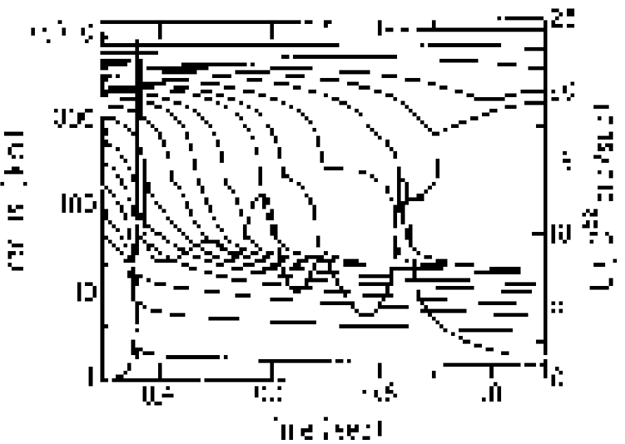
Fig. 31 shows time evolution of neutrino luminosities calculated by a simulation of the Livermore group [219]. This is based on a numerical progenitor model with mass $25M_{\odot}$ and a $2.05M_{\odot}$ core. The time evolution of $\nu_{e}$ luminosity is superimposed on the motion of mass shells in Fig. 31. The first $\nu_{e}$ peak is the neutronization burst, whose amplitude is drawn to be half the actual value in the figure. The next $O(1)$ sec is the matter accretion phase. The luminosities of $\nu_{e}$ and $\bar{\nu}_{e}$ are greater than that of $\nu_{x}$ because there are additional contributions to $\nu_{e}$ and $\bar{\nu}_{e}$ luminosities from the charged current interaction of the pair-annihilation of $e^{+}e^{-}$. As can be seen in Fig. 31, the neutrino luminosities increase when outer core matter accretes onto the protoneutron star. The final is the cooling phase of the protoneutron star, during which neutrino luminosities decrease exponentially with the neutrino diffusion timescale, $O(10)$ sec.

To summarize, neutrino emission from a supernova can divided into three phases. Because different mechanisms work during the three phases, they have different timescales and neutrino luminosities.

4.2.2 average energy

Figure 32: Time evolution of average neutrino energies [219]. Here $\nu,\bar{\nu}$ and $\mu$ denote $\nu_{e},\bar{\nu}_{e}$ and $\nu_{x}$, respectively, and the subscripts S and C stand for the calculation method. As neutronization of the protoneutron star proceeds, the difference between $\bar{\nu}_{e}$ and $\nu_{x}$ energies decreases.

Average energy of emitted neutrinos reflects the temperature of matter around the neutrinosphere. Interactions between neutrinos and matter are sufficiently strong inside the neutrinosphere so that thermal equilibrium is realized there. Since the temperature is lower in the outer region, neutrino average energy becomes lower as the radius of the neutrinosphere is larger. Then the problem is what determines the radius of the neutrinosphere. Basically, it is determined by the strength of interactions between neutrinos and matter.

Interactions between neutrinos and matter are,

$$\nu_{e}+n\leftrightarrow e^{-}+p,$$ (126)

$$\bar{\nu}_{e}+p\leftrightarrow e^{+}+n,$$ (127)

$$\nu+e^{\pm}\leftrightarrow\nu+e^{\pm},$$ (128)

$$\nu+N\leftrightarrow\nu+N.$$ (129)

Here it should be noted that the reactions (126) and (127) are relevant only to $\nu_{e}$ and $\bar{\nu}_{e}$, respectively. Furthermore, although all flavors interact with matter through the reaction (128), interactions for $\nu_{e}$ and $\bar{\nu}_{e}$ are contributed from both the neutral and charged current, while that for $\nu_{x}$ is contributed only from the neutral current. Interaction (129) occurs equally to all flavors. Therefore, interactions of $\nu_{e}$ and $\bar{\nu}_{e}$ are stronger than those of $\nu_{x}$. Because there are more neutrons than protons in the protoneutron star, $\nu_{e}$ couples stronger to matter than $\bar{\nu}_{e}$. Thus, it is expected that average energies of neutrinos have the following inequality:

$$\langle E_{\nu_{e}}\rangle<\langle E_{\bar{\nu}_{e}}\rangle<\langle E_{\nu_{x}}\rangle.$$ (130)

Although this hierarchy would be a robust prediction of the current supernova theory, it is highly difficult to estimate the differences of the average energies without detailed numerical simulations.

Fig. 32 shows time evolution of average neutrino energies obtained from the Livermore simulation [219]. We can see the hierarchy of neutrino average energies, Eq. (130). The difference between $\bar{\nu}_{e}$ and $\nu_{x}$ energies decreases in time because number of protons decreases as neutronization of the protoneutron star proceeds.

The differences of average energies are important particularly for neutrino oscillation. As an extreme case, neutrino oscillation does not affect neutrino spectra at all if all flavors have exactly the same energy spectrum. However, prediction of neutrino spectra by numerical simulation is highly sensitive and model-dependent although the qualitative feature, Eq. (130), is confirmed by a lot of simulations. Simulations by the Livermore group [219, 352] predict relatively large differences of average energies, while simulations of protoneutron star cooling by Suzuki predict much smaller differences [318, 301].

4.2.3 energy spectrum

The position of the neutrinosphere is determined by the strength of the interactions between neutrinos and matter. However, since the cross sections of the interactions depend on neutrino energy, the neutrinosphere has a finite width even for one flavor. Therefore, the energy spectra of neutrinos are not simple blackbodies. Because neutrinos with lower energies interact relatively weakly with matter, their neutrinospheres have smaller radii compared to those of high-energy neutrinos. As a result, the energy spectrum has a pinched shape compared to the Fermi-Dirac distribution.

Figure 33: Energy spectra of $\bar{\nu}_{e}$ at different times and the Fermi-Dirac distribution with the same average energies [340]. The chemical potentials of the Fermi-Dirac distributions are set to zero.

Figure 34: Time-integrated energy spectra [340].

Fig. 34 shows energy spectra of $\bar{\nu}_{e}$ at different times and the Fermi-Dirac distribution with the same average energies [340]. We can see the pinched Fermi-Dirac distribution at each time. Time-integrated energy spectra are shown in Fig. LABEL:fig:integrated_spe.

In the literature, the neutrino spectrum is sometimes parameterized in several forms. One popular way to parametrize is called a ”pinched” Fermi-Dirac spectrum (e.g. [210]),

$$F^{0}_{\alpha}(E)=\frac{L_{\alpha}}{F(\eta_{\alpha})T_{\alpha}^{4}}\frac{E^{2}}{e^{E/T_{\alpha}-\eta_{\alpha}}+1},$$ (131)

where $L_{\alpha}$ and $T_{\alpha}$ are the luminosity and effective temperature of $\nu_{\alpha}$, respectively, and $\eta_{\alpha}$ is a dimensionless pinching parameter. The normalization factor $F(\eta_{\alpha})$ is

$$F(\eta_{\alpha})\equiv\int^{\infty}_{0}\frac{x^{3}}{e^{x-\eta_{\alpha}}+1},$$ (132)

where $F(0)=7\pi^{4}/120\sim 5.68$. Their typical values obtained from numerical simulations are,

$$\langle E_{\bar{e}}\rangle=(14-22){\rm MeV},~{}~{}~{}\frac{\langle E_{x}\rangle}{\langle E_{\bar{e}}\rangle}=(1.1-1.6),~{}~{}~{}\frac{\langle E_{e}\rangle}{\langle E_{\bar{e}}\rangle}=(0.5-0.8),$$ (133)

$$\frac{L_{e}}{L_{x}}=(0.5-2),~{}~{}~{}\frac{L_{\bar{e}}}{L_{x}}=(0.5-2),$$ (134)

$$\eta_{e}=(0-3),~{}~{}~{}\eta_{\bar{e}}=(0-3),~{}~{}~{}\eta_{x}=(0-2).$$ (135)

Note that the average energy depends on both $T_{\alpha}$ and $\eta_{\alpha}$, and for $\eta_{\alpha}=0$ we have $\langle E_{\alpha}\rangle\sim 3.15T_{\alpha}$.

On the other hand, Keil et al. suggested the following form [170, 171],

$$F^{0}_{\alpha}(E)=\frac{L_{\alpha}}{\langle E_{\alpha}\rangle}\frac{\beta_{\alpha}^{\beta_{\alpha}}}{\Gamma(\beta_{\alpha})}\left(\frac{E}{\langle E_{\alpha}\rangle}\right)^{\beta_{\alpha}-1}\exp{\left(-\beta_{\alpha}\frac{E}{\langle E_{\alpha}\rangle}\right)},$$ (136)

where $L_{\alpha}$ and $E_{\alpha}$ denote the flux normalization and average energy, respectively, and $\beta_{\alpha}$ is a dimensionless parameter that relates to the width of the neutrino spectrum and typically takes on values $3.5-6$. It should be noted that these quantities are dependent on both the flavor and time. Spectra obtained from numerical simulations are well fitted by

$$\langle E_{e}\rangle=12{\rm MeV},~{}~{}~{}\langle E_{\bar{e}}\rangle=15{\rm MeV},~{}~{}~{}\langle E_{x}\rangle=24{\rm MeV},$$ (137)

$$\frac{L_{e}}{L_{x}}=2.0,~{}~{}~{}\frac{L_{\bar{e}}}{L_{x}}=1.6,$$ (138)

for the ones by the Livermore group and

$$\langle E_{e}\rangle=12{\rm MeV},~{}~{}~{}\langle E_{\bar{e}}\rangle=15{\rm MeV},~{}~{}~{}\langle E_{x}\rangle=(15-18){\rm MeV},$$ (139)

$$\frac{L_{e}}{L_{x}}=(0.5-0.8),~{}~{}~{}\frac{L_{\bar{e}}}{L_{x}}=(0.5-0.8),$$ (140)

for the ones by the Garching group which will be mentioned in the next section.

4.2.4 recent developments

Figure 35: (a) Position of the accretion front as a function of time. (b) Neutrino luminosities and rms energies as functions of time. In both figures, thick and thin lines show result from AGILE-BOLTZTRAN and VERTEX, respectively. The differences in the neutrino results are mainly indirect consequences of the approximate treatment of general relativity in the VERTEX simulation. [201]

Around neutrinosphere and shock front, neutrinos strongly couple the dynamics of different layers on short propagation time scales so that neither diffusion nor free streaming is a good approximation in this region. An accurate treatment of the neutrino transport and neutrino-matter interactions therefore are important not only for obtaining reliable neutrino spectra but also for following the dynamics of supernova correctly. It requires to solve energy- and angle-dependent Boltzmann transport equation, which is an extremely tough job. However, recent growing computer capability has made it possible to solve the Boltzmann equation in consistent with hydrodynamics [256, 197, 198, 265, 338, 201]. The result of simulations of several groups agree that spherically symmetric models with standard microphysical input fail to explode by the neutrino-driven mechanism.

In [201], Liebendörfer et al. gave a direct and detailed comparison between two independent codes of neutrino radiation-hydrodynamics, AGILE-BOLTZTRAN of the Oak Ridge-Basel group and VERTEX of the Garching group. Fig. 35 shows (a) the position of the accretion front as a function of time, and (b) the neutrino luminosities and rms energies as functions of time. The two codes are reasonably consistent as to the position of the accretion front. The differences in the neutrino results are mainly indirect consequences of the approximate treatment of general relativity in the VERTEX simulation. It can be seen that differences of rms neutrino energies are,

$$\langle E_{\bar{\nu}_{e}}\rangle-\langle E_{\nu_{e}}\rangle\sim 2-3{\rm MeV},~{}~{}~{}\langle E_{\nu_{x}}\rangle-\langle E_{\bar{\nu}_{e}}\rangle\sim 3-4{\rm MeV}.$$ (141)

However, since recent sophisticated simulations have not succeeded in explosion, it is conservative to consider that we do not have definite quantitative predictions about neutrino spectra.

Despite of the advent of the sophisticated simulations, traditional ones by the Livermore group are still useful for neutrino oscillation study of supernova neutrinos. This is because the latter has a great advantage that it covers the full evolution from the collapse over the explosion to the Kelvin-Helmholtz cooling phase of the newly formed neutron star, while the former covers typically at most 1 sec.

4.3 Neutrino Oscillation

4.3.1 overview

Observation of supernova neutrinos can give us information on deep inside of supernova which cannot be seen by electromagnetic waves. However, in general, neutrinos do not reach the earth as they were produced at the core due to neutrino oscillation. As in the case of the solar neutrino, resonant neutrino oscillation occurs in the star. In the current case, however, there are two resonance points involving three generations of neutrino because neutrinos of all three flavors are produced in the supernova and the core density is sufficiently high.

A key point in the three-generation resonance is the mass hierarchy of neutrino. Because there are three generation, there are two mass differences, which are obtained by several experiments as

$$\Delta m_{12}^{2}\approx 8\times 10^{-5}{\rm eV}^{2},$$

$$\Delta m_{13}^{2}\approx\Delta m_{23}^{2}\approx 2\times 10^{-3}{\rm eV}^{2}.$$ (142)

As was discussed in section 3.4.6, there are two ways to order these two mass difference: one is normal hierarchy, for which $m_{1}^{2}\approx m_{2}^{2}\ll m_{3}^{2}$, and another is inverted hierarchy, for which $m_{3}^{2}\ll m_{1}^{2}\approx m_{2}^{2}$.

The two resonance points are called H-resonance which occurs at denser region and L-resonance which occurs at less dense region. Because the resonance density is proportional to the mass difference of the two involved mass eigenstates (see Eq. (82)), H-resonance and L-resonance correspond to $\Delta m_{13}^{2}$ and $\Delta m_{12}^{2}$, respectively. Likewise, the involved mixing angles are $\theta_{13}$ and $\theta_{12}$ for H- and L-resonance, respectively. Thus, adiabaticities at the two resonance points depend on the following parameters:

$${\rm H-resonance~{}at~{}higher~{}density}\rightarrow\Delta m_{13}^{2},\theta_{13},$$ (143)

$${\rm L-resonance~{}at~{}lower~{}density}\rightarrow\Delta m_{12}^{2},\theta_{12}.$$ (144)

The situation is quite different for the two mass hierarchies. If the mass hierarchy is normal, there are two resonances in the neutrino sector, while there is one resonance in both the neutrino and anti-neutrino sector for the inverted mass hierarchy. The schematic views of the two situations are shown in Fig. 36. The vertical line corresponds to vacuum and (anti-)neutrino sector is right (left) hand side of it. Here it should be noted that $\nu_{e}$ and $\bar{\nu}_{e}$ become effectively heavier and lighter, respectively, in matter if neutral-current contributions to the effective mass are subtracted. As can be seen in Fig. 36, L-resonance always occurs in the neutrino sector, while H-resonance occurs in the neutrino sector for the normal hierarchy and in the anti-neutrino sector for the inverted hierarchy.

Figure 36: Resonance schemes for normal mass hierarchy (left) and inverted hierarchy (right).

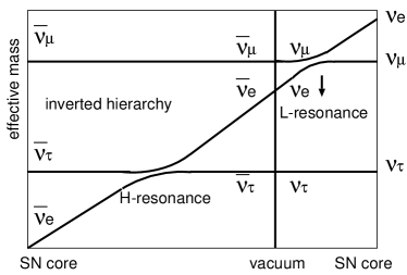
Neutrinos produced at the core have energy spectra which reflect the physical state of the core. Then neutrino oscillation changes the spectra according to the adiabaticities of the resonances. Since the adiabaticities depend on the density profile of the progenitor star and neutrino oscillation parameters, neutrino spectra observed at the earth are determined by:

• spectra at the core,

• density profile of the progenitor star,

• neutrino oscillation parameters (mixing angles, mass differences and mass hierarchy).

If we observe supernova neutrinos, a mixture of these information will be obtained. The former two of the three directly reflect the explosion mechanism of supernova, of which we have the basic picture as we discussed in section 2. However, since we have not succeeded in reproduce an explosion with a numerical simulation and we have not observed supernova neutrinos besides the small number of events (19 events) from SN1987A, it would be conservative to think that our understanding of the explosion mechanism, especially quantitative understanding, is incomplete. Thus, if we want to extract information on neutrino oscillation parameters, we have to conduct an analysis based on qualitative features of supernova neutrinos such as,

• $\nu_{e}$ emission by the neutronization burst,

• differences in the average energies and fluxed between flavors.

However, as we discuss later, number of the neutronization burst events would not be statistically sufficient unless supernova occurs several persec from the earth. Anyway, supernova is a unique source to probe neutrino oscillation parameters as is implied by the comparison to other neutrino sources (Table 6). Supernova neutrinos have quite different features from those of other sources so that useful information which cannot be obtained from other experiments is expected to be obtained.

Table 6: Comparison of some neutrino sources.

neutrino source	solar	atmospheric	supernova
production site	solar center	atmosphere	supernova core
flavor	${\nu}_{e}$	$\nu_{e},\nu_{\mu},\bar{\nu}_{e},\bar{\nu}_{\mu}$	${\nu}_{e},{\bar{\nu}}_{e},{\nu}_{x}$
energy	$\sim 10$ MeV	$\sim 1$ GeV	$10\sim 70$ MeV
resonance	once	none	twice
distance	1AU	10km	10kpc
		$\sim 10^{4}$km	(Galactic center)

On the other hand, if we want information on supernova itself, we have to subtract the effect of neutrino oscillation. Some of the neutrino oscillation parameter, such as 2 mass differences, $\theta_{12}$ and $\theta_{23}$, have been obtained with excellent accuracies by recent experiments as we saw in section 3.4.6. However, only a loose constraint has been obtained on $\theta_{13}$ and we have no idea on the mass hierarchy. Therefore it is not straightforward to obtain the intrinsic property of supernova neutrinos.

4.3.2 resonance points

As we saw in Eq. (82), the resonance density is,

$$\rho_{\rm res}=1.3\times 10^{6}{\rm g}~{}{\rm cm}^{-3}\cos{2\theta}\left(\frac{0.5}{Y_{e}}\right)\left(\frac{10{\rm MeV}}{E_{\nu}}\right)\left(\frac{\Delta m^{2}}{1{\rm eV}^{2}}\right),$$ (145)

from which, knowing the approximate values of the mass differences Eq. (142), the densities of H- and L-resonance regions are obtained as,

$$\rho_{\rm H}\approx(1-10)\times 10^{3}~{}{\rm g}~{}{\rm cm}^{-3},$$ (146)

$$\rho_{\rm L}\approx(20-200)~{}{\rm g}~{}{\rm cm}^{-3}.$$ (147)

We show a density profile of a progenitor star with mass $15M_{\odot}$ just before the core collapse in Fig. 38, which is based on a numerical model by Woosley and Weaver [356, 317]. Electron fraction is also shown in Fig. 38 for reference. As the figure shows, the resonance regions are far from the core:

$$r_{\rm H}\approx(0.05-0.1)R_{\odot},$$ (148)

$$r_{\rm L}\approx(0.1-0.2)R_{\odot}.$$ (149)

Therefore, it is conventional to assume that the dynamics of supernova is not affected by neutrino oscillation. Also it has often been assumed that the shock wave does not affect the structure of the region where the resonances occur so that static models of progenitor star have often been used to analyze neutrino oscillation. In fact, as we discuss later, shock wave reaches the resonance region in $O(1)$ sec and can change the adiabaticity of the resonances.

Figure 37: Density profile of a progenitor star with $15M_{\odot}$ just before core collapse [356, 317]. Also shown corresponding layers.

Figure 38: Electron-fraction profile of a progenitor star with $15M_{\odot}$ just before core collapse [356, 317].

4.3.3 conversion in supernova

Here we give a general discussion on flavor conversion in supernova following [78]. Our purpose here is to express neutrino fluxes at the surface of the star in terms of the original fluxes. Let us denote the original flux of flavor $\alpha$ at the core as $F^{0}_{\alpha}$. Because $\nu_{\mu},\nu_{\tau},\bar{\nu}_{\mu}$ and $\bar{\nu}_{\tau}$ interact with matter almost equally in supernova, their fluxes can also be considered to be equal and we define

$$F^{0}_{x}\equiv F^{0}_{\mu}=F^{0}_{\tau}=F^{0}_{\bar{\mu}}=F^{0}_{\bar{\tau}}$$ (150)

as the non-electron neutrino flux. For possible difference in $\nu_{\mu}$ and $\nu_{\tau}$ fluxes, see [3].

Although three-generation resonance is complicated in general, the hierarchy of the two mass-squared differences and the smallness of $U_{e3}$ simplify it substantially so that the two resonances can be considered to be two two-generation resonances [181, 182, 229]:

$$P^{\rm total}_{\nu_{e}\rightarrow\nu_{e}}=P^{\rm H}_{\nu_{e}\rightarrow\nu_{e}}\times P^{\rm L}_{\nu_{e}\rightarrow\nu_{e}}.$$ (151)

neutrino sector

For extremely high densities as in supernova core ($\rho\gg\rho_{\rm H},\rho_{\rm L}$), all mixings are suppressed so that the flavor eigenstates coincide with the eigenstates in the medium:

$$\nu_{3,{\rm m}}=\nu_{e},~{}~{}~{}\nu_{2,{\rm m}}=\nu_{\tau^{\prime}},~{}~{}~{}\nu_{1,{\rm m}}=\nu_{\mu^{\prime}}.$$ (152)

Correspondingly, the original fluxes of the eigenstates in medium are written as,

$$F^{0}_{3,{\rm m}}=F^{0}_{e},~{}~{}~{}F^{0}_{2,{\rm m}}=F^{0}_{\tau^{\prime}}=F^{0}_{x},~{}~{}~{}F^{0}_{1,{\rm m}}=F^{0}_{\mu^{\prime}}=F^{0}_{x}.$$ (153)

We now want to calculate the fluxes of mass eigenstates at the surface of the star assuming normal hierarchy. They will be written in terms of the original fluxes $F^{0}_{\alpha},(\alpha=e,\mu,\tau)$ and flip probabilities at the H- and L-resonances $P_{\rm H}$ and $P_{\rm L}$. First let us consider the fate of $F^{0}_{e}$. At the H-resonance, a fraction $P_{\rm H}$ of $F^{0}_{e}$ flip to lighter state $\nu_{2,{\rm m}}$ and $(1-P_{\rm H})$ remain to be $\nu_{3,{\rm m}}$. Among the $\nu_{2,{\rm m}}$ with flux $P_{\rm H}F^{0}_{e}$, a fraction $P_{\rm L}$ flip to the lightest state $\nu_{1,{\rm m}}$ and $(1-P_{\rm L})$ remain to be $\nu_{2,{\rm m}}$. As a consequence,

$$F^{0}_{e}\Longrightarrow\left\{\begin{array}[]{l}F_{1}:P_{\rm L}P_{\rm H}F^{0}_{e}\\ F_{2}:(1-P_{\rm L})P_{\rm H}F^{0}_{e}\\ F_{3}:(1-P_{\rm H})F^{0}_{e}\end{array}\right..$$ (154)

In the same way, $F_{i}$ are contributed from $\nu_{\mu^{\prime}}$ and $\nu_{\tau^{\prime}}$ as,

$$F^{0}_{\mu^{\prime}}\Longrightarrow\left\{\begin{array}[]{l}F_{1}:(1-P_{\rm L})F^{0}_{\mu^{\prime}}\\ F_{2}:P_{\rm L}F^{0}_{\mu^{\prime}}\\ F_{3}:0\end{array}\right.,~{}~{}~{}F^{0}_{\tau^{\prime}}\Longrightarrow\left\{\begin{array}[]{l}F_{1}:P_{\rm L}(1-P_{\rm H})F^{0}_{\tau^{\prime}}\\ F_{2}:(1-P_{\rm L})(1-P_{\rm H})F^{0}_{\tau^{\prime}}\\ F_{3}:P_{\rm H}F^{0}_{\tau^{\prime}}\end{array}\right..$$ (155)

Summing all the contributions, we obtain

$$F_{1}=P_{\rm L}P_{\rm H}F^{0}_{e}+(1-P_{\rm L}P_{\rm H})F^{0}_{x},$$ (156)

$$F_{2}=(1-P_{\rm L})P_{\rm H}F^{0}_{e}+(1-P_{\rm H}+P_{\rm L}P_{\rm H})F^{0}_{x},$$ (157)

$$F_{3}=(1-P_{\rm H})F^{0}_{e}+P_{\rm H}F^{0}_{x},$$ (158)

which are rewritten as,

$$F_{i}=a_{i}F^{0}_{e}+(1-a_{i})F^{0}_{x},$$ (159)

where

$$a_{1}=P_{\rm L}P_{\rm H},~{}~{}~{}a_{2}=(1-P_{\rm L})P_{\rm H},~{}~{}~{}a_{3}=1-P_{\rm H}.$$ (160)

Because the mass eigenstates are the eigenstates of the Hamiltonian in vacuum, they propagate independently to the earth. Further, their coherence is lost on the way to the earth so that the neutrinos arrive at the surface of the earth as incoherent fluxes of the mass eigenstates.

Taking into account the neutrino mixing, the net flux of $\nu_{e}$ is, upto the geometrical factor $1/4\pi L^{2}$,

$$F_{e} = \sum_{i}\left|U_{ei}\right|^{2}F_{i}$$ (161)

$$= F^{0}_{e}\sum_{i}\left|U_{ei}\right|^{2}a_{i}+F^{0}_{x}\left(1-\sum_{i}\left|U_{ei}\right|^{2}a_{i}\right)$$

$$= pF^{0}_{e}+(1-p)F^{0}_{x},$$

where we used the unitarity condition $\sum_{i}\left|U_{ei}\right|^{2}=1$ and the ”total survival probability of $\nu_{e}$”, $p$, is defined as,

$$p \equiv \left|U_{ei}\right|^{2}a_{i}$$ (162)

$$= \left|U_{e1}\right|^{2}P_{\rm L}P_{\rm H}+\left|U_{e2}\right|^{2}(1-P_{\rm L})P_{\rm H}+\left|U_{e3}\right|^{2}(1-P_{\rm H}).$$

Since the total flux is conserved, that is,

$$F^{0}_{e}+2F^{0}_{x}=F_{e}+2F_{x},$$ (163)

we obtain the net flux of $\nu_{x}$ as

$$F_{\mu}+F_{\tau}=2F_{x}=(1-p)F^{0}_{e}+(1+p)F^{0}_{x}.$$ (164)

Thus the fluxes at the surface of the earth can be expressed by the original fluxes and the survival probability $p$. Here it should be noted that not only the fluxes but also the survival probability depend on the neutrino energy.

So far, we have assumed the normal hierarchy. In fact, the case with the inverted hierarchy reduces the same expressions with $P_{\rm H}=1$.

anti-neutrino sector

Next we consider the antineutrino sector. Again, the flavor eigenstates coincide with the eigenstates in the medium at the core with sufficiently high densities:

$$\bar{\nu}_{3,{\rm m}}=\bar{\nu}_{\tau^{\prime}},~{}~{}~{}\bar{\nu}_{2,{\rm m}}=\bar{\nu}_{\mu^{\prime}},~{}~{}~{}\bar{\nu}_{1,{\rm m}}=\bar{\nu}_{e},$$ (165)

so that the original fluxes of the eigenstates in the medium are given by,

$$F^{0}_{\bar{3},{\rm m}}=F^{0}_{\bar{\tau}^{\prime}},~{}~{}~{}F^{0}_{\bar{2},{\rm m}}=F^{0}_{\bar{\mu}^{\prime}}=F^{0}_{x},~{}~{}~{}F^{0}_{\bar{1},{\rm m}}=F^{0}_{\bar{e}}=F^{0}_{x}.$$ (166)

Because the small mixing angle $\theta_{e3}$ is further suppressed in the medium, the $\bar{\nu}_{e}\leftrightarrow\bar{\nu}_{3}$ transitions are negligible, Also, the state $\bar{\nu}_{3}$ is so far from the level crossing that it propagates adiabatically, that is, $\bar{\nu}_{\tau}^{\prime}\rightarrow\bar{\nu}_{3}$. The other two states can flip through H-resonance for the inverted hierarchy. (For a possible L-resonance of anti-neutrino sector, see [292].) In the same way as the neutrino sector, we obtain,

$$F_{\bar{e}}=\bar{p}F^{0}_{\bar{e}}+(1-\bar{p})F^{0}_{x},$$ (167)

$$F_{\bar{\mu}}+F_{\bar{\tau}}=2F_{x}=(1-\bar{p})F^{0}_{\bar{e}}+(1+\bar{p})F^{0}_{x}.$$ (168)

where

$$\bar{p}=\left|U_{e1}\right|^{2}\bar{P}_{\rm H}+\left|U_{e3}\right|^{2}(1-\bar{P}_{\rm H}),$$ (169)

is the effective survival probability of $\bar{\nu}_{e}$. For the normal hierarchy, $\bar{P}_{\rm H}=1$.

summary

Summarizing the considerations above, the neutrino fluxes can be written as,

$$\left(\begin{array}[]{c}F_{e}\\ F_{\bar{e}}\\ 4F_{x}\end{array}\right)=\left(\begin{array}[]{ccc}p&0&1-p\\ 0&\bar{p}&1-\bar{p}\\ 1-p&1-\bar{p}&2+p+\bar{p}\end{array}\right)\left(\begin{array}[]{c}F^{0}_{e}\\ F^{0}_{\bar{e}}\\ F^{0}_{x}\end{array}\right)$$ (170)

with survival probabilities,

$$p=\left|U_{e1}\right|^{2}P_{\rm L}P_{\rm H}+\left|U_{e2}\right|^{2}(1-P_{\rm L})P_{\rm H}+\left|U_{e3}\right|^{2}(1-P_{\rm H}),$$ (171)

$$\bar{p}=\left|U_{e1}\right|^{2}\bar{P}_{\rm H}+\left|U_{e3}\right|^{2}(1-\bar{P}_{\rm H}),$$ (172)

which depend on neutrino energy, neutrino oscillation parameters and mass scheme.

4.3.4 survival probabilities

In the previous section, we obtained an general expression of neutrino fluxes at the surface of the earth in terms of original fluxes and survival probabilities, which can be expressed by the conversion probabilities at the two resonances and oscillation parameters.

The survival probabilities $p$ and $\bar{p}$ can be calculated from the following Schrödinger-like equation,

$$i\frac{d}{dt}\left(\begin{array}[]{c}\nu_{e}\\ \nu_{\mu}\\ \nu_{\tau}\end{array}\right)=H(t)\left(\begin{array}[]{c}\nu_{e}\\ \nu_{\mu}\\ \nu_{\tau}\end{array}\right),$$ (173)

where the effective Hamiltonian is given by

$$H(t)=U\left(\begin{array}[]{ccc}0&0&0\\ 0&\Delta m^{2}_{12}/2E&0\\ 0&0&\Delta m^{2}_{13}/2E\end{array}\right)U^{-1}+\left(\begin{array}[]{ccc}A(t)&0&0\\ 0&0&0\\ 0&0&0\end{array}\right),$$ (174)

and matter function $A(t)$ is given by

$$A(t)=\sqrt{2}G_{F}n_{e}(t).$$ (175)

When the two resonances are perfectly adiabatic or non-adiabatic, the situation is simple. Let us first estimate the adiabaticies of the two resonances. If we assume the density profile of the progenitor star as

$$\rho(r)=\rho_{0}r^{-n},$$ (176)

the adiabaticity parameter $\gamma$, defined in Eq. (90), is written as,

$$\gamma=\frac{1}{2n}\frac{\sin^{2}{2\theta}}{(\cos{2\theta})^{1+1/n}}\left(\frac{\Delta m^{2}}{E}\right)^{1-1/n}\left(\frac{2\sqrt{2}G_{F}Y_{e}\rho_{0}}{m_{p}}\right)^{1/n}.$$ (177)

Adopting an approximate value $n=-3$ in the mantle, we have

$$\gamma = 9\times 10^{3}\frac{\sin^{2}{2\theta_{13}}}{(\cos{2\theta_{13}})^{4/3}}\left(\frac{\Delta m_{13}^{2}}{2\times 10^{-3}{\rm eV}^{2}}\right)^{2/3}\left(\frac{10{\rm MeV}}{E}\right)^{2/3}~{}~{}~{}({\rm for~{}H-resonance})$$ (179)

$$= 10^{3}\frac{\sin^{2}{2\theta_{12}}}{(\cos{2\theta_{12}})^{4/3}}\left(\frac{\Delta m_{12}^{2}}{8\times 10^{-5}{\rm eV}^{2}}\right)^{2/3}\left(\frac{10{\rm MeV}}{E}\right)^{2/3},~{}~{}~{}$$

$$({\rm for~{}L-resonance})$$

Substituting the mixing angle obtained from solar neutrino observation into Eq. (179), it is seen that the L-resonance is perfectly adiabatic for an energy range of supernova neutrino ($E=1-100{\rm eV}$). On the other hand, for the current constraint on $\theta_{13}$, the H-resonance can be either perfectly adiabatic or perfectly non-adiabatic.

Figure 39: Survival probabilities of $\nu_{e}$ (left) and $\bar{\nu}_{e}$ (right) in the progenitor star [321]. Survival probabilities depend drastically on the mass scheme (normal or inverted) and the value of $\theta_{13}$ (Large or Small). When the resonances are sufficiently adiabatic or non-adiabatic, difference in neutrino energy leads to just difference of the position of resonance.

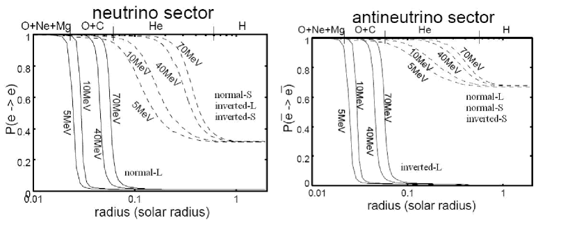
Takahashi et al. followed the evolution of survival probabilities, $P_{\nu_{e}\rightarrow\nu_{e}}$ and $P_{\bar{\nu}_{e}\rightarrow\bar{\nu}_{e}}$, in [325, 321]. Their calculations were performed by solving the Schrödinger equation (173) numerically along the density profile of the progenitor star given in Fig. 38. Fig. 39 shows the evolution of the survival probabilities with sufficiently large (L, $\sin^{2}{2\theta_{13}}>10^{-3}$) and small (S, $\sin^{2}{2\theta_{13}}<10^{-5}$) values of $\theta_{13}$ [321]. Here ”normal-L” means a model with sufficiently large $\theta_{13}$ and normal mass hierarchy. As can be seen the survival probabilities depend drastically on the mass scheme and the value of $\theta_{13}$. It is also seen that difference in neutrino energy leads to just difference of the position of resonance because the resonances are sufficiently adiabatic or non-adiabatic. Here it should be noted that mass hierarchy is not important when $\theta_{13}$ is sufficiently small because, in this case, the H-resonance is perfectly non-adiabatic, which is equivalent to the absence of the H-resonance.

4.3.5 neutrino spectra

Figure 40: Original neutrino spectra [340] used in [321].

Figure 41: Original evolution of neutrino flux [340] used in [321].

With survival probabilities obtained in section 4.3.4, information of detector, which will be discussed in section 4.5, and original neutrino fluxes, we can calculate number of events at the detector. In [321], original neutrino fluxes calculated by a realistic model of a collapse-driven supernova by the Lawrence Livermore group [352, 340] was used and is shown in Figs. 41 and 41. Figs. 44, 44 and 44 show time-integrated energy spectra and time evolution of the number of neutrino events at SK and SNO. Event number of each interaction is also shown in Tables 7 and 8. The distance between the earth and the supernova was set to 10 kpc, which corresponds to the galactic center. As in section 4.3.4, ”normal” and ”inverted” represent the mass hierarchy and ”L” and ”S” mean that $\theta_{13}$ is enough large and small for the H-resonance to be perfectly adiabatic and non-adiabatic, respectively.

With a supernova at 10 kpc, SK will have an enormous number of events, which is mostly $\bar{\nu}_{e}p$ events, and make a statistical study possible. SNO will have much smaller events than SK but it can count the number of $\nu_{e}$s. Thus it is expected that we can obtain many useful information by combining data from the two detectors. However, at both detectors, event number of neutronization burst will be rather small.

Figure 42: Time-integrated energy spectra (left) and the time evolution of the number of neutrino events (right) at SK. Only $\bar{\nu}_{e}p$ CC interaction, which is the dominant event at SK, is taken into account [321].

Figure 43: Time-integrated energy spectra (left) and the time evolution of the number of $\nu_{e}d$ events (right) at SNO. Neutronization burst is suppressed for normal-S, inverted-L and inverted-S, and absent for normal-L [321].

Figure 44: Time-integrated energy spectra (left) and the time evolution of the number of $\bar{\nu}_{e}d$ events (right) at SNO [321].

Table 7: Number of events at SK

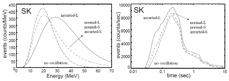
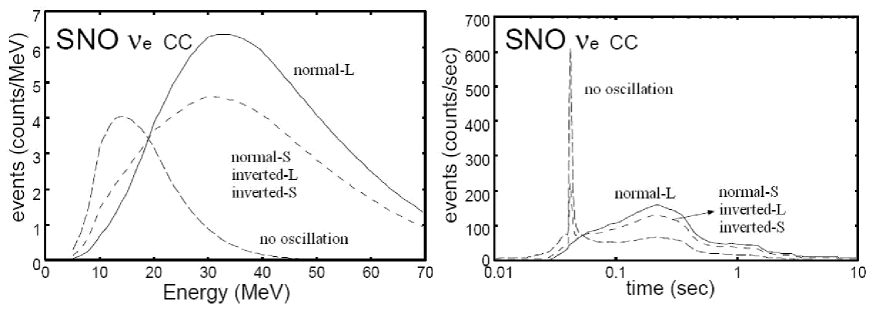
hierarchy	normal		inverted
$\theta_{13}$	large	small	large	small	no osc
$\bar{\nu}_{e}p$	9459	9427	12269	9441	8036
$\nu_{e}e^{-}$	186	171	171	171	132
$\bar{\nu}_{e}e^{-}$	46	46	56	46	42
$\nu_{x}e^{-}$	98	98	77	98
$O\nu_{e}$	297	214	297	214	31
$O\bar{\nu}_{e}$	160	158	296	159	92
total	10245	10114	13084	10129	8441
burst	15.7	16.7	20.1	16.7	12.4

Table 8: Number of events (CC) at SNO

hierarchy	normal		inverted
$\theta_{13}$	large	small	large	small	no osc
$\nu_{e}d{\rm(CC)}$	237	185	185	185	68
$\bar{\nu}_{e}d{\rm(CC)}$	118	117	190	117	82
total	355	302	375	302	150
burst	0.6	1.1	1.1	1.1	2.1

In general, neutrino oscillation makes the $\nu_{e}$ and $\bar{\nu}_{e}$ spectra harder, since the original average energies of $\nu_{e}$ and $\bar{\nu}_{e}$ are smaller than that of $\nu_{x}$. In other words, neutrino oscillation produces high energy $\nu_{e}$ and $\bar{\nu}_{e}$ from $\nu_{x}$. As a result, the number of high-energy events increases and that of low-energy events decreases. The boundary between high energy and low energy is around 20 MeV. Note that the amounts of these increase and decrease depend on the adiabaticity parameters, and therefore the neutrino oscillation parameters, as can be seen in Figs. 44, 44 and 44. This feature can be used as a criterion for the magnitude of the neutrino oscillation effects. In [321], the following simple ratios were introduced as a criterion:

$$R=\frac{{\rm number\;of\;events\;at}\;20{\rm MeV}<E_{\nu}<70{\rm MeV}}{{\rm number\;of\;events\;at}\;5{\rm MeV}<E_{\nu}<20{\rm MeV}}.$$ (180)

The ratios at SK and SNO are plotted in the left of Fig. 45. In this figure, only $\nu_{e}d$ CC events are taken into account for $R_{\rm SNO}$ and error bars represent the statistical errors only. The ratios $R_{\rm SK}$ and $R_{\rm SNO}$ can be considered as estimators of neutrino conversion at neutrino sector and anti-neutrino sector, respectively. As can be seen, the ratios will give a reasonable implication for the mass hierarchy and the value of $\theta_{13}$, especially SK is expected to give valuable information on $\theta_{13}$ with its large event number in case of inverted hierarchy. However the mass hierarchy cannot be distinguished if $\theta_{13}$ is very small. Note that the $\nu_{e}$ flux and the $\bar{\nu}_{e}$ flux contain essentially different information about the neutrino oscillation parameters. For example, inverted-L and inverted-S are distinguishable from $\bar{\nu}_{e}$ events, but they are not distinguishable from $\nu_{e}$ events.

Figure 45: (left) Ratios of high-energy to low-energy events at SK and SNO. (right) Dependence of the ratios on $\sin^{2}{\theta_{13}}$. In both figures, only $\nu_{e}d$ events are taken into account for $R(SNO)$ and error bars represent the statistical errors only [321].

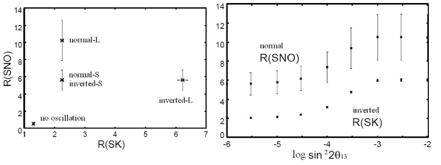
To this point, we have considered only two extreme cases with perfectly adiabatic and non-adiabatic H-resonances. It is also interesting to investigate the intermediate cases. In the right of Fig. 45 the $\theta_{13}$ dependences of $R_{\rm SK}$ and $R_{\rm SNO}$ are plotted. Here it should be note that $R_{\rm SK}$ and $R_{\rm SNO}$ vary only in the cases of inverted and normal hierarchies, respectively, as expected from Figs. 44, 44 and 44. In the case of the normal hierarchy, it would be difficult to determine the value of $\theta_{13}$, due to the small event number at SNO and large statistical errors, but it will give a hint whether it is very large or very small. In the case of the inverted hierarchy, the overlap of the error bars is small even in the intermediate cases. If $\theta_{13}$ is rather large ($\sin^{2}{2\theta_{13}}>10^{-3}$), these rations will give useful information of the mass hierarchy.

4.3.6 Earth effects

Figure 46: Neutrinos passing through the earth before reaching a detector.

Figure 47: Path lengths in the earth of neutrinos from the galactic center to various detectors as functions of the time of the day. The distance in the earth is normalized by the earth diameter.

We have discussed neutrino oscillation in supernova and its effects on neutrino signal at detectors. Here we will consider matter effect inside the earth. Actually, neutrinos can pass through the earth before reaching the detector depending on the configuration of the supernova, the earth and the detector (Fig. 47). Fig. 47 shows path lengths in the earth of neutrinos from the galactic center to various detectors as functions of the time of the day. The distance in the earth is normalized by the earth diameter. As one can see, at any time of the day, at least one detector among SK (Japan), SNO (Canada) and LVD (Italy) observes neutrinos which have experienced the earth matter.

The earth matter can have extra effects on the supernova neutrino spectra and observation/non-observation of them can give us further information on neutrino oscillation parameters and original neutrino fluxes. First we give a general discussion on the earth matter effect following again [78].

Figure 48: Amplitude of the earth matter effect $\xi\sin^{2}{2\theta_{12}}/[(\xi-\cos{2\theta_{12}})^{2}+\sin^{2}{2\theta_{12}}]$ as a function of $\xi$. Here we set $\sin^{2}{\theta_{12}}=0.3$. Anti-neutrino sector is shown in the negative energy region.

Figure 49: Fluxes of $\nu_{e}$ with the earth effect (dashed line) and without the earth effect (solid). Here it is assumed that $\nu_{e}$s propagate 4,000 km in matter with the density of the earth core.

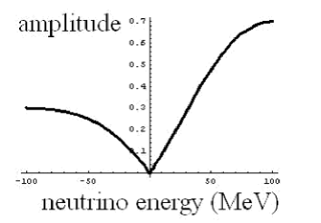
First, we consider the neutrino sector assuming the normal hierarchy. But it is equivalent for the inverted hierarchy if we set $P_{\rm H}=0$ and also for the anti-neutrino sector with the normal and inverted hierarchy if we set $P_{\rm H}=P_{\rm L}=0$ and $P_{\rm L}=0$, respectively. Flux of $\nu_{e}$ at the surface of the earth, $F_{e}$, is written as Eq. (161),

$$F_{e}=\sum_{i}|U_{ie}|^{2}F_{i}=pF^{0}_{e}+(1-p)F^{0}_{x},$$ (181)

where $F_{i}$ is the flux of $i$-th mass eigenstate $\nu_{i}$ and $p$ is the survival probability of $\nu_{e}$ defined in Eq. (162). Now let $P_{ie}$ be the probability that a $\nu_{i}$ entering the earth reaches the detector as a $\nu_{e}$. Then the flux of $\nu_{e}$ at the detector, $F^{\rm D}_{e}$, is,

$$F^{\rm D}_{e}=\sum_{i}P_{ie}F_{i}.$$ (182)

Rewriting $F_{i}$s by the original fluxes $F^{0}_{\alpha}$ using Eq. (159), we obtain,

$$F^{\rm D}_{e} = F^{0}_{e}\sum_{i}a_{i}P_{ie}+F^{0}_{x}\left(1-\sum_{i}a_{i}P_{ie}\right)$$ (183)

$$= p^{\rm D}F^{0}_{e}+(1-p^{\rm D})F^{0}_{x},$$

where we have used the unitarity condition $\sum_{i}P_{ie}=1$ in the first line and,

$$p^{\rm D}\equiv\sum_{i}a_{i}P_{ie},$$ (184)

is the effective survival probability of $\nu_{e}$ at the detector. The earth effect can be expressed by the difference between $F_{e}$ and $F^{\rm D}_{e}$:

$$F^{\rm D}_{e}-F_{e}=(p^{\rm D}-p)\left(F^{0}_{e}-F^{0}_{x}\right).$$ (185)

The difference of the survival probabilities are computed as,

$$p^{\rm D}-p = \sum_{i}a_{i}(P_{ie}-|U_{ie}|^{2})$$ (186)

$$= (1-2P_{\rm L})P_{\rm H}(P_{2e}-|U_{2e}|^{2})+(1-P_{\rm H}-P_{\rm L}P_{\rm H})(P_{3e}-|U_{3e}|^{2}),$$

where $\sum_{i}P_{ie}=1$ was used. Because the earth density is rather low and the mixing angle $\theta_{13}$ is known to be small, we can neglect the second term. Thus we have,

$$F^{\rm D}_{e}-F_{e}=(1-2P_{\rm L})P_{\rm H}(P_{2e}-|U_{2e}|^{2})\left(F^{0}_{e}-F^{0}_{x}\right).$$ (187)

Now let us evaluate the factor $(P_{2e}-|U_{2e}|^{2})$. For simplicity, we assume a constant density and two-flavor oscillation. Remembering that the flavor eigenstates can be written by both vacuum mass eigenstates and eigenstates in matter, that is,

$$\left(\begin{array}[]{c}\nu_{e}\\ \nu_{\mu}\end{array}\right)=U\left(\begin{array}[]{c}\nu_{1}\\ \nu_{2}\end{array}\right)=U_{\rm m}\left(\begin{array}[]{c}\nu_{1,{\rm m}}\\ \nu_{2,{\rm m}}\end{array}\right),$$ (188)

where $U$ and $U_{\rm m}$ are mixing matrix in vacuum and in matter, respectively, we have

$$\left(\begin{array}[]{c}\nu_{1}\\ \nu_{2}\end{array}\right) = U^{-1}U_{\rm m}\left(\begin{array}[]{c}\nu_{1,{\rm m}}\\ \nu_{2,{\rm m}}\end{array}\right)$$ (193)

$$= \left(\begin{array}[]{cc}\cos{(\theta_{12,{\rm m}}-\theta_{12})}&\sin{(\theta_{12,{\rm m}}-\theta_{12})}\\ -\sin{(\theta_{12,{\rm m}}-\theta_{12})}&\cos{(\theta_{12,{\rm m}}-\theta_{12})}\end{array}\right)\left(\begin{array}[]{c}\nu_{1,{\rm m}}\\ \nu_{2,{\rm m}}\end{array}\right).$$ (198)

Now consider a neutrino which is initially a $\nu_{2}$ and enter the earth. The wave function evolves as,

$$\nu_{2}(z) = -\sin{(\theta_{12,{\rm m}}-\theta_{12})}\exp{\left(-i\frac{m_{1,{\rm m}}^{2}}{2E}z\right)}\nu_{1,{\rm m}}$$

$$+\cos{(\theta_{12,{\rm m}}-\theta_{12})}\exp{\left(-i\frac{m_{2,{\rm m}}^{2}}{2E}z\right)}\nu_{2,{\rm m}}$$

$$= -\exp{\left(-i\frac{m_{1,{\rm m}}^{2}}{2E}z\right)}\times$$

$$\left[\sin{(\theta_{12,{\rm m}}-\theta_{12})}\cos{\theta_{12,{\rm m}}}-\cos{(\theta_{12,{\rm m}}-\theta_{12})}\sin{\theta_{12,{\rm m}}}\exp{\left(-i\frac{\Delta m_{\rm m}^{2}}{2E}z\right)}\right]\nu_{e}$$

$$+\exp{\left(-i\frac{m_{1,{\rm m}}^{2}}{2E}z\right)}\times$$

$$\left[\sin{(\theta_{12,{\rm m}}-\theta_{12})}\sin{\theta_{12,{\rm m}}}+\cos{(\theta_{12,{\rm m}}-\theta_{12})}\cos{\theta_{12,{\rm m}}}\exp{\left(-i\frac{\Delta m_{\rm m}^{2}}{2E}z\right)}\right]\nu_{\mu}.$$

Then $P_{2e}$, the probability that a $\nu_{2}$ entering the earth is observed as a $\nu_{e}$ is,

$$P_{2e}=\sin^{2}{\theta_{12}}-\frac{\xi\sin^{2}{2\theta_{12}}}{(\xi-\cos{2\theta_{12}})^{2}+\sin^{2}{2\theta_{12}}}\sin^{2}{\left(\frac{\pi z}{\ell_{\rm osc,m}}\right)},$$ (200)

where $\xi$ is the dimensionless density parameter defined in Eq. (79),

$$\xi = \frac{2\sqrt{2}G_{F}n_{B}E}{\Delta m^{2}}$$ (201)

$$= 9.6\times 10^{-2}\left(\frac{Y_{e}\rho}{5{\rm g}~{}{\rm cm}^{-3}}\right)\left(\frac{E}{10{\rm MeV}}\right)\left(\frac{8\times 10^{-5}{\rm eV}^{2}}{\Delta m^{2}}\right),$$

and $\ell_{\rm osc,m}$ is the oscillation length in matter defined in Eq. (80),

$$\ell_{\rm osc,m} = \frac{\ell_{\rm osc}}{\sqrt{(\xi-\cos{2\theta})^{2}+\sin^{2}{2\theta}}}$$ (202)

$$= 3.1\times 10^{2}{\rm km}\frac{1}{\sqrt{(\xi-\cos{2\theta})^{2}+\sin^{2}{2\theta}}}\left(\frac{E}{10{\rm MeV}}\right)\times$$

$$\left(\frac{8\times 10^{-5}{\rm eV}}{\Delta m^{2}}\right).$$

Eventually, we have the final expression:

$$F^{\rm D}_{e}-F_{e} = (1-2P_{\rm L})P_{\rm H}\frac{\xi\sin^{2}{2\theta_{12}}}{(\xi-\cos{2\theta_{12}})^{2}+\sin^{2}{2\theta_{12}}}\times$$ (203)

$$\sin^{2}{\left(\frac{\pi z}{\ell_{\rm osc,m}}\right)}\left(F^{0}_{x}-F^{0}_{e}\right).$$

We can easily understand this expression. First of all, there must be a difference between the fluxes of $\nu_{e}$ and $\nu_{x}$ in order for neutrino oscillation to have any effects. Since flux of $\nu_{e}$ is larger and smaller than that of $\nu_{x}$ at lower and higher energies, respectively, the earth effect is expected to change sign at some critical energy where $F_{e}^{0}(E_{\rm crit})=F_{x}^{0}(E_{\rm crit})$. This critical energy is about 20 MeV in the simulation of the Livermore group.

Then there must also be a difference between the fluxes of $\nu_{1}$ and $\nu_{2}$ at the surface of the earth because we have neglected the contribution from the third generation. This fact is reflected in the factor $(1-2P_{\rm L})P_{\rm H}$: if $P_{\rm H}=0$, both $\nu_{1}$ and $\nu_{2}$ have the original spectrum of $\nu_{x}$ and if $P_{\rm H}=1/2$, both $\nu_{1}$ and $\nu_{2}$ have the same mixture of the original spectra of $\nu_{e}$ and $\nu_{x}$. Therefore it is expected that if $\theta_{13}$ is so large ($\sin^{2}{2\theta_{13}}>10^{-3}$) that the H-resonance is perfectly adiabatic, there is no earth matter effect on $\nu_{e}$ and $\bar{\nu}_{e}$ spectra for the normal and inverted hierarchy, respectively. Therefore, existence of the earth effect is determined by $\theta_{13}$ and the mass hierarchy:

• small $\theta_{13}$ $\rightarrow$ $\nu_{e}$ and $\bar{\nu}_{e}$

• large $\theta_{13}$ and normal hierarchy $\rightarrow$ $\bar{\nu}_{e}$

• large $\theta_{13}$ and inverted hierarchy $\rightarrow$ $\nu_{e}$

Thus observation/non-observation of the earth effects will give further information on neutrino parameters and mass hierarchy.

Finally, the remaining factor represents the magnitude of the earth matter effect which oscillates with an amplitude $|\xi\sin^{2}{2\theta_{12}}/[(\xi-\cos{2\theta_{12}})^{2}+\sin^{2}{2\theta_{12}}]|$ and with an oscillation length $\ell_{\rm osc,m}$. The amplitude is plotted in Fig. 49 as a function of $\xi$. Anti-neutrino sector is shown the negative energy region. As one can see, the earth matter effect will be larger for higher energies. Comparing the neutrino and anti-neutrino sector, it is expected that the earth effect in the neutrino sector is larger than that in the anti-neutrino sector because both the above amplitude and the difference of neutrino spectrum compared with $\nu_{x}$ are larger for $\nu_{e}$ than $\bar{\nu}_{e}$.

In Fig. 49, fluxes of $\nu_{e}$ with and without the earth effect are shown. Here it is assumed that $\nu_{e}$s propagate 4,000 km in matter with the density of the earth core. At low and high energies, $\nu_{e}$ flux increases and decreases, respectively, due to the earth effect. As is expected, the earth effect vanishes at the critical energy. Note also that there is a modulation in the spectrum, which is a unique feature of the earth effect and comes from the factor $\sin^{2}{(\pi z/\ell_{\rm osc,m})}$ in Eq. (203). This feature will be further discussed in the next section.

4.3.7 detection and implication from earth effect

Figure 50: Density profile of the earth [85].

Figure 51: Event spectra at SK and SNO with earth effect with some values of zenith angle and $\Delta m_{12}^{2}$ [320]. In the left row, $\Delta m_{12}^{2}$ is fixed to $2\times 10^{-5}{\rm eV}^{2}$ and, in the right row, zenith angle is fixed to zero. Only charged-current events are considered in the SNO spectra. The mixing angle $\theta_{13}$ is taken sufficiently small that the H-resonance is perfectly non-adiabatic.

Here we discuss the earth effects more in detail. Because the oscillation length is almost the same order of the earth radius, the earth effects depend highly on the path length of neutrinos inside the earth. The path length is determined by the position of detector on the earth, the direction of supernova and the time of the day. As we saw in Fig. 47, at least one detector among SK, SNO and LVD will observe neutrinos with the earth effect and at least one detector will observe neutrinos without the earth effect at anytime if a supernova occurs at the galactic center.

If we can see a supernova optically, its direction can be determined accurately. However, it is likely that the light from supernova is obscured by interstellar dust if the supernova occurs around the galactic center. Methods of direction determination by neutrinos are suggested and studied by several authors. One strategy is to use electron scattering events [BeacomFogel99]. As we will see in section 4.5, scattered electron in electron scattering event reflects the direction of the incident neutrino. In [9], the accuracy of the direction determination was estimated to be about 9 degree using expected event data at SuperKamiokande. Much better accuracy about $0.6^{o}$ is expected if a megaton water Cherenkov detector is available [336]. Another strategy is triangulation using time delay of neutrino signals at different neutrino detectors [47]. However, given the expected statistics, this method was shown to be not so effective [32].

As we discussed in the previous section, $\theta_{13}$ and the mass hierarchy determines the existence of the earth effects. Further, since the oscillation length depends on $\Delta m_{12}^{2}$, the spectral modulation due to the earth effects will be highly dependent on the value of $\Delta m_{12}^{2}$. In [320], the dependence of the earth effects on $\Delta m_{12}^{2}$ and the path length of neutrinos inside the earth was studied in detail. The computational method is essentially the same as that without the earth effects: the Schrödinger equation (173) needs to be solved along the density profile of the earth. The standard density profile of the earth is shown in Fig. 50 [85].

Fig. 51 shows event spectra at SK and SNO with earth effect with some values of zenith angle and $\Delta m_{12}^{2}$ [320]. In the left row, $\Delta m_{12}^{2}$ is fixed to $2\times 10^{-5}{\rm eV}^{2}$ and, in the right row, zenith angle is fixed to zero. It is seen that the spectral shape varies with the zenith angle and $\Delta m_{12}^{2}$. Since the oscillation length is shorter for larger $\Delta m_{12}^{2}$, the frequency of spectral modulation with respect to neutrino energy is larger for larger $\Delta m_{12}^{2}$. Thus, two detectors located at separate cites observe neutrinos with different energy spectra because their path lengths in the earth are different in general. Also, one can see that the earth effect at SK is smaller than that at SNO. This is because the dominant events at SK are $\bar{\nu}_{e}$ while both $\nu_{e}$ and $\bar{\nu}_{e}$ contribute to the signal at SNO.

Thus the detection of the earth effect will give us information on $\theta_{13}$, the mass hierarchy and $\Delta m_{12}^{2}$. There are basically two strategies for detecting the earth effect. One is to compare the neutrino fluxes at two or more sites and another is to identify the spectral modulation mentioned above. Because the earth effect is a rather small effect, the former strategy needs large detectors. On the other hand, the latter strategy needs only one detector although it must have a sufficient energy resolution to identify the spectral modulation.

Figure 52: Variation of the expected IceCube signal with neutrino earth-crossing length [76]. The signal is normalized to unity when no earth effect is present ($L=0$). The solid and dashed lines correspond to the accretion phase and cooling phase, respectively.

Figure 53: Contours of $N_{\rm SK}/N_{\rm IC}$ on the map of the sky projected on the earth [76]

.

Table 9: Regions in Fig. 53 for the earth effect in IceCube and Super-Kamiokande.

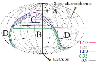
Region	Sky fraction	Neutrinos come from		$N_{\rm SK}/N_{\rm IC}$
		IceCube	Super-K
A	0.35	below	above	1.070
B	0.35	above	below	0.935
C	0.15	below	below	Fluctuations around 1
D	0.15	above	above	1

Comparison of neutrino flux at two detector was considered in [76]. This method is simple but the detectors must be enough large to accomplish statistically significant detection of the earth effect. They considered IceCube and SuperKamiokande, both of which are Cherenkov detectors. Because the dominant events come from $\bar{\nu}_{e}$ at both the detectors, the earth effects are relatively small. Fig. 53 shows the variation of the expected IceCube signal with neutrino earth-crossing length. The signal is normalized to unity when no earth effect is present ($L=0$). The solid and dashed lines correspond to the accretion phase and cooling phase, respectively. Here they used neutrino spectra with,

$$\langle E_{\bar{\nu}_{e}}^{0}\rangle=15{\rm MeV},~{}~{}~{}\langle E_{\nu_{x}}^{0}\rangle=17{\rm MeV},~{}~{}~{}\frac{F_{\bar{e}}^{0}}{F_{x}^{0}}=1.5,$$ (204)

for the accretion phase and,

$$\langle E_{\bar{\nu}_{e}}^{0}\rangle=15{\rm MeV},~{}~{}~{}\langle E_{\nu_{x}}^{0}\rangle=18{\rm MeV},~{}~{}~{}\frac{F_{\bar{e}}^{0}}{F_{x}^{0}}=0.8,$$ (205)

for the cooling phase, and neutrino mixing parameters they used $\Delta m_{12}^{2}=6\times 10^{-5}{\rm eV}^{2}$ and $\sin^{2}{2\theta_{12}}=0.9$.

Denoting the number of Cherenkov photon at IceCube as $N_{\rm IC}$ and the equivalent IceCube signal measured by SK as $N_{\rm SK}$, the contour of the ratio $N_{\rm SK}/N_{\rm IC}$ is shown in Fig. 53. The sky can be divided into four regions according to the direction of neutrinos at the two detectors (Table 9). As one can see, deviation of the ratio $N_{\rm SK}/N_{\rm IC}$ from unity is significant when either IceCube or SK observes neutrinos directly and the other observes neutrinos from below and the deviation is typically 0.07 in such cases. This deviation is rather large because, if a supernova explodes at 10 kpc from the earth, the statistical precision for the total neutrino energy deposition is about $0.2\%$ for the IceCube and $1\%$ for the SK. Further, such ideal cases is realized for about $70\%$ of the sky. Thus the geographical position of IceCube with respect to SK at a latitude of $36.4^{o}$ is well-suited for the detection of the earth effect through a combination of the signals.

The second possibility, making use of the spectral modulation, was pursued by Dighe et al. [77, 75]. Their basic idea is to Fourier-transform the ”inverse-energy” spectrum of the signal. As we saw in the previous section, the spectral modulation due to the earth effect comes from the following factor in Eq. (203),

$$F^{\rm D}_{e}-F_{e}\propto\sin^{2}{\left(\frac{\Delta m_{12,{\rm m}}^{2}z}{4E_{\nu}}\right)}.$$ (206)

Therefore the earth effect will have a clear peak in the power spectrum if it is Fourier-transformed with respect to $E^{-1}$. The position of the peak is determined by a factor $\Delta m_{12,{\rm m}}^{2}z$, that is, $\Delta m_{12}^{2}$, the density of the region which neutrinos propagate and the path length. It is important to note that the peak position is not affected by the primary neutrino spectra so that the value of $\Delta m_{12}^{2}$ can be determined accurately from the peak position independently of supernova model if we know the neutrino path length inside the earth.

To illustrate the effectiveness of their method, they consider a 32 kton scintillator detector and a megaton water Cherenkov detector. The major difference between the scintillation and the water Cherenkov detector is that the energy resolution of the scintillation detector is roughly six times better than that of the Cherenkov detector. Therefore even the volume of the SuperKamiokande will not be sufficient to identify the earth effect and much larger detector, HyperKamiokande (HK), is needed.

Figs. 55 and 55 show expected power spectra at the scintillator detector and HK, respectively, for different SN models, Garching (G) and Livermore (L), and distances traveled through the earth. Supernova is assumed to be 10 kpc from the earth and the power spectra are averaged over 1000 SN simulations. The left rows show the power spectra of neutrinos which propagate only in the earth mantle while the right rows correspond to those which propagate the earth core as well as the mantle.

A clear peak is seen in each figure in the left rows, corresponding to the assumed values of $\Delta m_{12}^{2}$, the mantle density, the average neutrino energy and the path length. The peak width reflects the finite energy resolution of the detectors and weak energy dependence of Eq. (203) besides the factor Eq. (206). The large power at small $k$ is the dominant contribution from the energy dependence of the neutrino spectra without the earth effect. On the other hand, if neutrinos propagate in both the mantle and core, multiple peaks appear as in the right rows of the figures corresponding to their densities and path lengths in them.

The Livermore model was used as a representative model of conventional simulations which predict relatively large average-energy differences between flavors. On the other hand, the Garching model, which treats neutrinos more carefully, predicts rather small average-energy differences between flavors. As we saw in the previous section, the earth effects as well as the effects of neutrino oscillation in supernova are larger for a case with larger average-energy differences. However, as seen in the figure, the peak positions are independent of the supernova models.

Figure 54: Averaged power spectra in the case of a large scintillator detector for different SN models, Garching (G) and Livermore (L), and distances traveled through the earth [75].

Figure 55: Same as the Fig. 55 but for the case of HK [75].

Figure 56: Left: Realistic spectrum from a single simulation. Right: Area distribution of the background (black) and the signal (red) obtained for a 32 kton scintillator detector and Garching model for $\eta=60$ [75].

Figure 57: Left: Comparison of $p_{95}$ and $p_{99}$ for the Garching (G) and Livermore (L) SN models in a 32 kton scintillator detector. Right: Comparison of $p_{95}$ in this large scintillator detector (SC) and in the case of a megaton water Cherenkov (HK), for the Garching model. From [75].

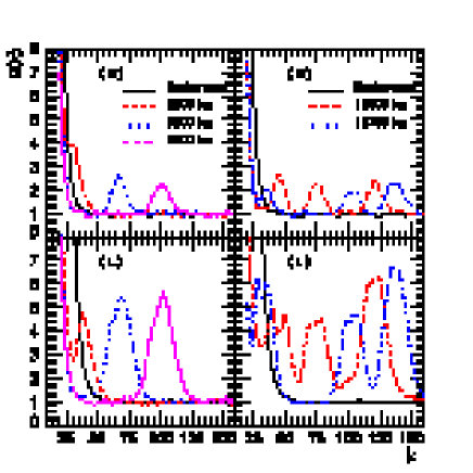
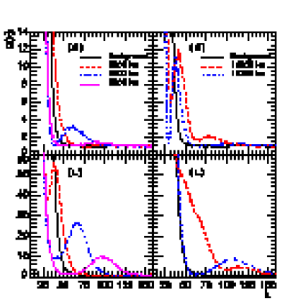
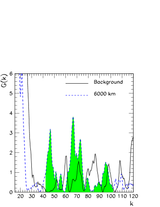
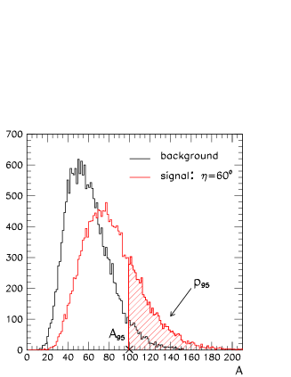
To quantify the effectiveness of their method, they introduced an algorithm to identify the peaks in the real world with the presence of background fluctuations. It is based on the integration of the area around the expected position of the peak. Once we know the neutrino path, we can calculate the position of the peaks. It is more robust to consider the area around the expected position of the peak than to look for the maximum in the height of the power spectrum, as shown in the left of Fig. 57. They considered, for a single peak case, the interval of integration $k_{\rm peak}\pm\Delta k$ with $\Delta k=30$, which is roughly the expected width of the peak. For a multiple peak case, they measure the area $k=40-160$.

Then we must consider the statistical significance of the result obtained. For this purpose, they compared the value of the measured area with the distribution of the area in the case of no earth effect. The right of Fig. 57 shows the area distribution of Monte Carlo simulations with and without the earth effect. Here $A_{95}\sim 100$ denote the area corresponding to $95\%$ C.L. detection of the earth effect. The problem is the probability that we have larger area than $A_{95}$, which is denoted by $p_{95}$. This probability depends on the distance traveled by the neutrinos through the earth, which is in turn determined by the location of the supernova in the sky. In Fig. 57, the probability as a function of the nadir angle $\eta$ of supernova is plotted. The passage through the core corresponds to $\eta<33^{o}$. The left is comparison of $p_{95}$ and $p_{99}$ for the Garching and Livermore SN models in a 32 kton scintillator detector. The right is comparison of $p_{95}$ in this large scintillator detector (SC) and in the case of a megaton water Cherenkov (HK), for the Garching model. As can be seen, this method is very effective if the average-energy differences of the original neutrino spectra are as large as predicted by the Livermore simulation, while the effectiveness decreases by half with the Garching simulation.

4.3.8 shock wave and neutrino oscillation

So far we have assumed the structure of supernova envelope to be static during $\sim 10{\rm sec}$ of neutrino emission. Actually, as pointed out by Schirato and Fuller [282] and studied further in [323, 211, 110, 337, 93], the shock wave produced at the bounce reaches the resonance regions in several seconds (left of Fig. 58) and can affect the adiabaticities of the resonances. This fact implies the possibility to probe the propagation of the shock wave by neutrino observation.

Figure 58: Left: Propagation of forward and reverse shocks with densities of H- and L-resonance regions [337]. The width of the density bands reflects the energy range of supernova neutrinos. Right: Schematic density profile in the presence of a forward and reverse shock wave with a contact discontinuity between them. Four key densities are denoted as $\rho_{\rm 1b},\rho_{\rm 2b},\rho_{\rm 2a}$ and $\rho_{\rm 1a}$ from dense to sparse region, which correspond to the edges of the forward and reverse shocks.

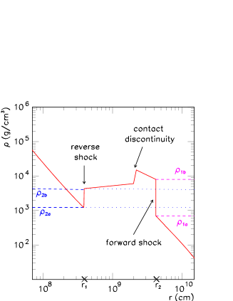
Before we discuss neutrino oscillation, let us summarize basic features of shock wave. While the shock sweeps the infalling matter, the gain region behind the shock is accelerated by the neutrinos from the neutron star to form the neutrino-driven wind. At the interface between this neutrino-driven wind and the shock-accerelated ejecta is formed a contact discontinuity, which is characterized by a density jump but continuous velocity and pressure. Even farther behind the forward shock, a reverse shock can appear due to the collision between the neutrino-driven wind and more slowly moving material. The forward and reverse shocks are sharp discontinuities where density, pressure and velocity change on the microscopic (sub-millimeter) scale of the ion mean free path. The right of Fig. 58 shows a schematic density profile in the presence of a forward and reverse shock wave with a contact discontinuity between them. The existence of the contact discontinuity and reverse shock seems to be a generic feature in supernova explosion according to recent numerical simulation. However, because the structure and time evolution of the shock wave depend on the detailed dynamics during the early stages of the supernova explosion, it is difficult to make an exact prediction. The situation becomes even more complicated if we consider non-spherical supernova explosion where violent convective instabilities and large anisotropies make the density structure chaotic, although the some generic features of the one-dimensional situation are retained. Here we discuss effects of shock propagation on neutrino oscillation in one-dimensional supernova following [337].

Figure 59: Left: Survival probability as a function of energy with $\cos^{2}{\theta_{12}}=0.7$. The dotted line corresponds to the probability based on the simple argument in the text while the solid line is based on a more realistic analytic evaluation in [337]. Right: Survival probability $\bar{p}(E,t)$ as a function of energy at different times averaging in energies with the energy resolution of Super-Kamiokande: for a profile with only a forward shock (left) and a profile with forward and reverse shock (right). At $t=5$ sec, $\bar{p}(E,t)$ including Earth matter effects for a zenith angle of $62^{o}$ is also shown with a black line. Both are from [337].

Figure 60: Upper and lower left: The average energy of $\bar{\nu}p\to ne^{+}$ events at a megaton water Cherenkov detector binned in time for simulations by the Livermore group (L) and the Garching group (G1 and G2). The average energy is assumed to be static and the error bars represent $1\sigma$ errors in any bin. Lower right: Time dependence of $\langle E_{e}\rangle$ for a profile with a forward and reverse shock for several values of $\tan^{2}{\theta_{13}}$ and for model L. Figures from [337].

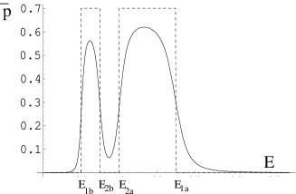
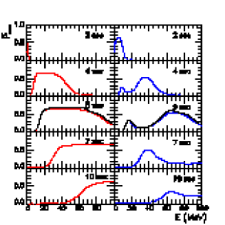
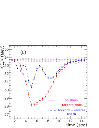
First, let us consider the survival probability of neutrinos which experience the H-resonance, that is, $\nu_{e}$s and $\bar{\nu}_{e}$ for the normal and inverted hierarchy, respectively. In this section, we assume the inverted hierarchy and consider $\bar{\nu}_{e}$. We can obtain a qualitative feature of the survival probability as a function of neutrino energy from the schematic density profile of the shock shown in the right of Fig. 58. In the figure, four key densities are denoted as $\rho_{\rm 1b},\rho_{\rm 2b},\rho_{\rm 2a}$ and $\rho_{\rm 1a}$ from dense to sparse region. They correspond to the edges of the forward and reverse shock: the density jumps from $\rho_{\rm 2a}$ to $\rho_{\rm 2b}$ at the reverse shock and from $\rho_{\rm 1b}$ to $\rho_{\rm 1a}$ at the forward shock. As we saw in Eq. (82), the resonance density is proportional to the neutrino energy,

$$\rho_{\rm res}=1.3\times 10^{3}{\rm g}~{}{\rm cm}^{-3}\cos{2\theta}\left(\frac{0.5}{Y_{e}}\right)\left(\frac{10{\rm MeV}}{E_{\nu}}\right)\left(\frac{\Delta m^{2}}{10^{-3}{\rm eV}^{2}}\right),$$ (207)

so that there are four energies whose resonance densities are the above four densities, $E_{\rm 1b},E_{\rm 2b},E_{\rm 2a}$ and $E_{\rm 1a}$ from lower to higher energies. Here it should be noted that the four densities are time-dependent and so are the four energies.

The essential point in the effect of shock propagation on neutrino oscillation is that the density gradient at the shocks is so steep that the resonance there tends to be non-adiabatic even if the mixing angle involved is rather large. Let us assume first that the resonance is completely non-adiabatic at the shocks and completely adiabatic elsewhere. The latter means that $\theta_{13}$ is sufficiently large. Then, a $\bar{\nu}_{e}$ with energy $E_{\rm 1b}<E<E_{\rm 2b}$ experiences the H-resonance three times, that is, behind the reverse shock, between the reverse and forward shock, and at the forward shock, which are adiabatic, adiabatic and non-adiabatic, respectively. The three resonances are equivalent to one non-adiabatic resonance. In the same way, we obtain the adiabaticities of resonances of various neutrino energies,

• $E<E_{\rm 1b}\Rightarrow$ adiabatic

• $E_{\rm 1b}<E<E_{\rm 2b}\Rightarrow$ adiabatic, adiabatic, non-adiabatic $\Rightarrow$ effectively non-adiabatic

• $E_{\rm 2b}<E<E_{\rm 2a}\Rightarrow$ adiabatic, non-adiabatic, non-adiabatic $\Rightarrow$ effectively adiabatic

• $E_{\rm 2a}<E<E_{\rm 1a}\Rightarrow$ non-adiabatic

• $E>E_{\rm 1a}\Rightarrow$ adiabatic

and the survival probability as a function of neutrino energy become like the left of Fig. 59. As one can see, there are two peaks in the survival probability, which result, as we will see later, in characteristic features in the time evolution of observed neutrino average energy and event number. Note that there will be only one peak without the reverse shock and that the behavior of the survival probability will become more complicated if the contact discontinuity is so sharp that resonance there is non-adiabatic. Anyway, since we assumed $\theta_{13}$ to be sufficiently large so that the survival probability is zero in absence of shock propagation, the effect of the shock can be thought to be to make the resonance more non-adiabatic effectively.

Because the shock propagate into low-density regions, the key densities decrease in time and so the key energies increase in time. The right of Fig. 59 shows the survival probability $\bar{p}(E,t)$ as a function of energy at different times averaging in energies with the energy resolution of Super-Kamiokande: for a profile with only a forward shock (left) and a profile with forward and reverse shock (right). At $t=5$ sec, $\bar{p}(E,t)$ including earth matter effects for a zenith angle of $62^{o}$ is also shown with a black line. It can be seen than there is only one peak without the reverse shock and are two peaks with both the reverse and forward shocks and the peaks shift to high-energy regions as the shock propagates, as expected.

Upper and lower left of Fig. 60 show the average energy of $\bar{\nu_{e}}p\to ne^{+}$ events binned in time for simulations by the Livermore group (L) and the Garching group (G1 and G2). Magenta, red and blue lines correspond to a static density profile, a profile with only a forward shock and with forward and reverse shock, respectively. The error bars are $1\sigma$ statistical errors assuming a megaton water Cherenkov detector. As one can see, there are some dips in the time evolution of the average energy: one dip with only forward shock and double dips with both forward and reverse shock. This characteristic feature is the direct result of the dips in the survival probability in Fig. 59 and can be seen in every SN model. Lower right of Fig. 60 is the time dependence of the average energy for a profile with a forward and reverse shock for several values of $\tan^{2}{\theta_{13}}$ and for model L. It is seen that the dips are smaller for smaller values of $\tan^{2}{\theta_{13}}$. This can be understood by remembering that the propagation of the shock waves through the resonance region tends to make the resonance more non-adiabatic effectively. When $\tan^{2}{\theta_{13}}$ is small, the H-resonance is non-adiabatic even without the shock and then the shock has no effect on neutrino oscillation.

Figure 61: Left: Total number of events as a function of time for a static density profile and a profile with only forward shock and with both forward and reverse shock. Right: Same as the left but the energy range is restricted to $E=40\pm 5{\rm MeV}$. The error bars are statistical errors expected in a megaton water Cherenkov detector. Both are from [337].

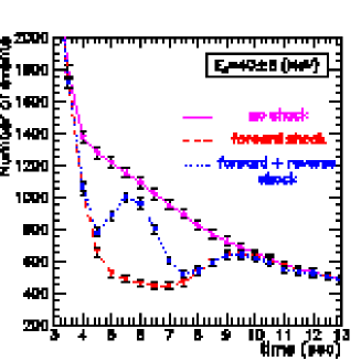
The imprint of the shock waves can also seen in the time evolution of the event number. The left of Fig. 61 shows the total number of events as a function of time for a static density profile and a profile with only forward shock and with both forward and reverse shock. As one can see, a dip can be seen in the presence of both the forward and reverse shocks. This is even striking if the energy range is restricted to $E=40\pm 5{\rm MeV}$ as can be seen in the right of Fig. 61.

Thus, if $\theta_{13}$ is sufficiently large ($\tan^{2}{\theta_{13}}>10^{-5}$), dips appear in the time evolution the neutrino average energy and event number, which would be relatively model-independent. A megaton water Cherenkov detector, like the HyperKamiokande, can probe the shock wave propagation efficiently if the mass hierarchy is inverted one so that the H-resonance occurs at the anti-neutrino sector.

4.3.9 toward model-independent predictions

Figure 62: Density profiles (left) and scale height $n_{e}/|dn_{e}/dr|$ of stars just before supernova explosion with initial mass $15M_{\odot},20M_{\odot},40M_{\odot}$ and $75M_{\odot}$ [322].

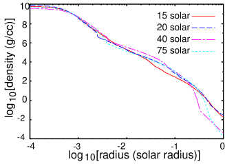
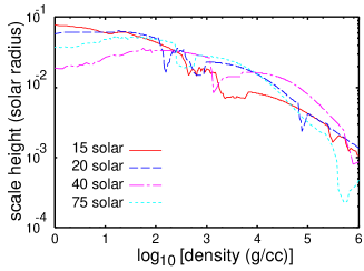
While type Ia supernovae have rather universal features as far as we observe them, core-collapse supernovae seem to have a wide variety in luminosity and spectrum. Since this will reflect the diversity of the presupernova structure, neutrino emission will also be dependent on the physical state of the progenitor star. Some important physical quantities about the progenitor star will include its mass, metalicity, magnetic field and rotation, whose effects on neutrino emission are still unclear. If we want to extract information about neutrino oscillation parameters, the effects of these supernova parameters on the neutrino emission and dynamics of neutrino oscillation must be studied and some model-independent analyses are required. In [322], Takahashi et al. studied the effect of initial mass of a progenitor star on the neutrino emission and neutrino oscillation. Then some input-physics dependences of neutrino emission were studied in [162] concentrating on neutronization-burst signal. Here we review [322] and summarize [162] briefly.

The mass of the progenitor star affects the neutrino oscillation signature of supernova neutrinos through differences in both the mantle and core structures. The density profile of the progenitor star, especially of the mantle, is important because it is related to the dynamics of neutrino flavor conversion. On the other hand, the structure of the iron core at the collapse determines the characteristics of the neutrino burst, e.g., the average energy and luminosity for each flavor.

Let us first discuss the density profile of a progenitor star. In numerical simulations of supernova, the initial condition is a star just before the collapse whose structure is often given by a numerical presupernova model, which is obtained by following the evolution of a massive star. The evolution of a massive star is significantly affected by mass loss due to a stellar wind, which we still do not have a definite understanding. Indeed, the mass loss can become so strong for a star with initial mass more than about 35 $M_{\odot}$ and solar metalicity that the entire hydrogen envelope can be lost prior to the explosion of the star. It is suggested in [355] that the maximum in the final mass is about 20 $M_{\odot}$. Thus, a massive star just before the supernova explosion may have a universal structure independent of the initial mass of the star. The final density profiles of stars with various initial masses just before the collapse are shown in the left of Fig. 62 [317]. As is expected, they are similar to each other.

The density profile of the star comes into the adiabaticity parameter as the scale height $n_{e}/|dn_{e}/dr|$. A smaller scale height, that is, a steeper density profile results in less adiabatic resonance. The scale heights of stars with various initial masses, calculated from the density profiles shown in the left of Fig. 62, are given in the right of Fig. 62 as functions of the density. The scale heights vary significantly, but, at the densities relevant for the resonances, differences between different initial masses are factors of 2 or 3.

Figure 63: Left: Evolution of survival probabilities $P(\nu_{e}\rightarrow\nu_{e})$ as functions of radius for different progenitor models. Upper and lower curves correspond to neutrino energies of 40 MeV and 5 MeV, respectively. Right: Energy dependence of survival probability $P(\nu_{e}\rightarrow\nu_{e})$ for different progenitor models. Also shown are the perfectly adiabatic and non-adiabatic cases for the H-resonance.

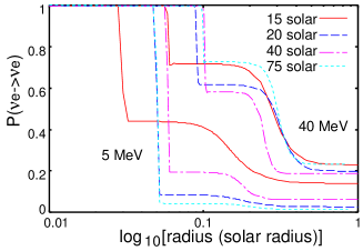
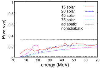
In the left of Fig. 63, the evolution of the survival probability $P(\nu_{e}\to\nu_{e})$ is shown. The neutrino energies on the plot are 5 MeV and 40 MeV and we set $\sin^{2}{2\theta_{13}}=10^{-4}$. The H-resonance radii and the final probabilities can be quite different for different progenitors and neutrino energies. The observationally important quantity is the final probability and this is shown in the right of Fig. 63 as a function of the neutrino energy. The differences are not so small, about $O(10)\%$ at all energies. But if $\sin^{2}{2\theta_{13}}$ is so large or very small that H-resonance is perfectly adiabatic or non-adiabatic, respectively, difference in scale height will not affect the neutrino conversion probabilities.

Next we consider the difference in core structure. As was stated in the above, massive stars experience significant mass loss. For current empirical mass loss rates, all solar-metalicity stars initially more massive than about $35\ M_{\odot}$ are thought to become hydrogen-free objects of roughly $5M_{\odot}$ at the end of their thermonuclear evolution. The corresponding upper limit to the mass of the final iron core is about $2M_{\odot}$ [355].

As mentioned in subsection 2.2, the mass of the iron core is determined roughly by the Chandrasekhar mass. For a zero-temperature and constant $Y_{e}$, its Newtonian structure is given by,

$$M_{\rm Ch0}=5.83Y^{2}_{e}M_{\odot}.$$ (208)

However, there are numerous corrections, some of which are large [339]. To the first approximation, the non-zero entropy of the core is important and

$$M_{\rm Ch}\sim M_{\rm Ch0}\left[1+\left(\frac{s_{e}}{\pi Y_{e}}\right)^{2}\right],$$ (209)

where

$$s_{e}=0.50\left(\frac{\rho}{10^{10}{\rm g/cc}}\right)^{-1/3}\left(\frac{Y_{e}}{0.42}\right)^{2/3}\left(\frac{T}{1{\rm MeV}}\right)$$ (210)

is the electronic entropy per baryon. More massive stars have higher entropy and contain larger iron cores on average. However, this general tendency is moderated by the loss and redistribution of entropy that occurs during the late burning stages. Thus, the mass of the iron core as a function of the initial mass will be somewhat uncertain in that a small change in the initial mass results in a large difference in the iron core mass. According to [355], the mass of the iron core is $1.2(1.4)-1.6M_{\odot}$ when the initial mass is between $10(20)M_{\odot}$ and $40M_{\odot}$. This weak dependence of the iron core mass on the ZAMS progenitor mass leads to a somewhat universal neutrino burst.

Fig. 64 shows the evolution of the average neutrino energy and number luminosity in the early phase up to 200 milliseconds after bounce. The calculation is based on dynamical models of core-collapse supernovae in one spatial dimension, employing a Boltzmann neutrino radiation transport algorithm, coupled to Newtonian Lagrangean hydrodynamics and a consistent high-density nuclear equation of state. Details of these simulations are described in [338]. As can be seen, the major features of the early neutrino burst are almost independent of the initial mass.

Combined with the discussion on the scale height above, we conclude that the mantle structure and the features of the neutrino burst depend little on the initial mass of the progenitor star if $\sin^{2}{2\theta_{13}}<10^{-5}$ or $\sin^{2}{2\theta_{13}}>10^{-3}$. On one hand, this means that we can not easily obtain information about the initial mass from observations of neutrinos during the first 200 milliseconds after bounce. On the other hand, this situation is desirable for extracting information about the neutrino parameters.

In [162], Kachelriess studied dependence of neutronization burst on input neutrino physics in numerical simulation, as well as progenitor mass. They found neutronization burst to be relatively independent of the progenitor mass, electron capture rate and equation of state at high densities. Especially, uncertainties in the number of neutronization-burst events due to the input physics was estimated to be less than $10\%$. This feature can be used not only to probe neutrino parameters such as $\theta_{13}$ and the mass hierarchy but also to determine the distance to the supernova. The latter is important because it is likely that the supernova is optically obscured by dust if it occurs around the galactic center. Their estimation is that distance to the next galactic supernova is determined with a $6\%$ error if we have a megaton water Cherenkov detector.

As we have discussed above, effects of some of neutrino parameters and input physics on supernova neutrinos and their oscillation have been studied so far. Fortunately to particle physics, the progenitor mass, electron capture rate and equation of state have relatively small effects on neutrinos and we will not suffer from uncertainties due to them. However, analyses so far are rather restricted to one-dimensional supernova, that is, we do not understand multi-dimensional effects such as magnetic field and rotation. This is because multi-dimensional simulation with sufficiently detailed treatment of the neutrino physics is still challenging now and much progress in this field is indispensable.

Figure 64: Left: Evolution of the number flux at the Earth of neutrinos from a supernova by a progenitor with initial masses $15M_{\odot},20M_{\odot},40M_{\odot}$ and $75M_{\odot}$ at a distance of 10 kiloparsecs. Right: Evolution of neutrino average energies. In all figures, time at the bounce is set to zero.

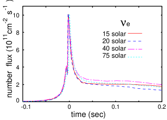
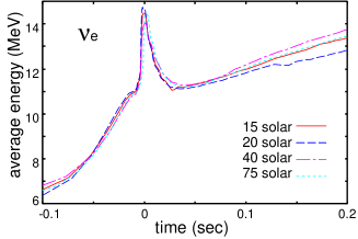
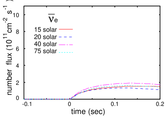
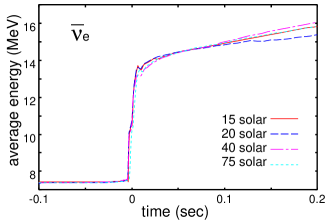
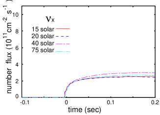
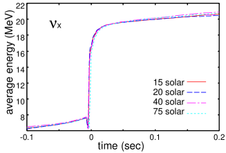
4.4 Neutrinos from SN1987A

On February 23 in 1987, a supernova was found in the Large Magellanic Cloud. This is the closest supernova from us since a galactic supernova in 17th century. From various analyses, this supernova, SN1987A, was identified as a type II supernova whose progenitor star is a blue giant with mass $M\sim 10M_{\odot}$ at 50 kpc. Here we review the basic facts of neutrinos from SN1987A and their implication.

4.4.1 observational facts

Table 10: Arrival times of neutrinos, energies of prompt electrons and angles between momenta of neutrinos and corresponding prompt electrons at Kamiokande II and IMB.

KII				IMB
event	time	energy	angle	event	time	energy	angle
	(sec)	(MeV)	(deg)		(sec)	(MeV)	(deg)
1	0.000	20.0 $\pm$ 2.9	18 $\pm$ 18	1	0.000	38 $\pm$ 7	80 $\pm$ 10
2	0.107	13.5 $\pm$ 3.2	40 $\pm$ 27	2	0.412	37 $\pm$ 7	44 $\pm$ 15
3	0.303	7.5 $\pm$ 2.0	108 $\pm$ 32	3	0.650	28 $\pm$ 6	56 $\pm$ 20
4	0.324	9.2 $\pm$ 2.7	70 $\pm$ 30	4	1.141	39 $\pm$ 7	65 $\pm$ 20
5	0.507	12.8 $\pm$ 2.9	135 $\pm$ 23	5	1.562	36 $\pm$ 9	33 $\pm$ 15
6	1.541	35.4 $\pm$ 8.0	32 $\pm$ 16	6	2.684	36 $\pm$ 6	52 $\pm$ 10
7	1.728	21.0 $\pm$ 4.2	30 $\pm$ 18	7	5.010	19 $\pm$ 5	42 $\pm$ 20
8	1.915	19.8 $\pm$ 3.2	38 $\pm$ 22	8	5.582	22 $\pm$ 5	104 $\pm$ 20
9	9.219	8.6 $\pm$ 2.7	122 $\pm$ 30
10	10.433	13.0 $\pm$ 2.6	49 $\pm$ 26
11	12.439	8.9 $\pm$ 1.9	91 $\pm$ 39

Figure 65: Arrival times and estimated energies of neutrinos observed at Kamiokande II and IMB [134].

Figure 66: Detection efficiencies at Kamiokande II [134] and IMB [41].

Just after the discovery of SN1987A by optical observations, it was expected that neutrinos from such a close supernova must have been detected. Actually Kamiokande II [133, 134] and Irvine-Michigan-Brookhaven detector (IMB) [36, 41] observed 11 and 8 events, respectively. (For possible detection of neutrinos at Baksan, see [5].)

Table 10 shows the arrival times of neutrinos, energies of prompt electrons and angles between momenta of neutrinos and corresponding prompt electrons at Kamiokande II and IMB. Arrival times and estimated energies of neutrinos observed at the Kamiokande II and IMB are plotted in Fig. 66. From this figure, one might think that neutrinos detected at the IMB have higher energies than those detected at the Kamiokande II. But it is not obvious because we have to consider the difference in detection efficiencies showed in Fig. 66. As one can see, the Kamiokande II had a high efficiency at more than 20 MeV while the IMB was not effective to detect low-energy neutrinos. We summarize basic information on the observed neutrinos below.

duration

The duration of neutrino events is 12.4 sec at the Kamiokande II and 5.6 sec at the IMB. This is consistent with the diffusion timescale of neutrino, about 10 sec, discussed in 4.2. Thus it is confirmed that neutrinos are confined in the protoneutron star and escape by diffusion.

angular distribution of events

Since both the Kamiokande II and IMB are water Cherenkov detectors, main events come from $\bar{\nu}_{e}p\to e^{+}n$ which has about hundred times larger cross section than that of electron scattering $\nu e^{-}\to\nu e^{-}$. A positron is emitted isotropically in $\bar{\nu}_{e}p\to e^{+}n$ while an electron scattered by a neutrino has a forward peak. Angular distribution in Table 10 confirms these arguments.

Let us focus on the first event at the Kamiokande II. In this event the primary electron is emitted forward. The probability that an electron, which has an isotropic distribution, is emitted forward inside $20^{o}$ is $3\%$, which leads to the expectation value of 0.6 for total event number of 19. On the other hand, as we saw in Table 7, event number of electron scattering is about $5\%$ of that of $\bar{\nu}_{e}p\to e^{+}n$ event. Thus, it is not obvious which reaction the first event came from. If the electron scattering is the case, $\nu_{e}$ is the most likely for the event because $\nu_{e}$ has the largest cross section in electron scattering.

neutronization burst?

If the first event at the Kamiokande II was $\nu_{e}$ event, it is possible that the $\nu_{e}$ is emitted during the neutronization burst. However, the event number from the neutronization burst was estimated to be about 0.01 in [280]. Thus it is unlikely that the first event at the Kamiokande II was from the neutronization burst.

neutrino temperature and luminosity

Neutrinos from supernova have roughly a thermal distribution though they do not exactly. The effective temperature and luminosity of the observed $\bar{\nu}_{e}$ were estimated by several authors [11, 152]. They are roughly consistent with each other and give,

$$T_{\bar{\nu}_{e}}=(3-4){\rm MeV},~{}~{}~{}L_{\bar{\nu}_{e}}=(3-6)\times 10^{52}{\rm erg}.$$ (211)

If we assume that all flavors have the same luminosity, the total neutrino luminosity is about $3\times 10^{53}{\rm erg}$. This is about the same as the binding energy of a neutron star, which indicates that the current supernova theory is roughly correct.

4.4.2 constraints on neutrino properties

Observational feature of the neutrinos from SN1987A can be summarized as follows:

• Duration of the neutrino events is about 12 sec

• Temperature of $\bar{\nu}_{e}$ is about $(3-4)$ MeV

• Neutrino total energy is roughly the same as the binding energy of a neutron star

We can put constraints on any new physics, unknown processes and exotic particles which lead to any contradictions with the above observational facts. Here we will discuss topics related to neutrinos.

mass

If neutrinos have mass, neutrinos with different energies have different velocities,

$$v_{\nu}\approx 1-\frac{m_{\nu}^{2}}{2E_{\nu}^{2}},$$ (212)

so that the propagation time from the SN1987A to the earth are also different. Denoting the departure and arrival times as $t_{\rm d}$ and $t_{\rm a}$, respectively, the propagation time can be written as

$$t_{\rm a}-t_{\rm d}=\frac{D}{v_{\nu}}\approx D\left(1+\frac{m_{\nu}^{2}}{2E_{\nu}^{2}}\right),$$ (213)

where $D\sim 50{\rm kpc}$ is the distance between SN1987A and the earth. Therefore the difference in the propagation times of two neutrinos is,

$$|\Delta t_{\rm a}-\Delta t_{\rm d}|=\frac{1}{2}Dm_{\nu}^{2}\frac{|E_{1}^{2}-E_{2}^{2}|}{E_{1}^{2}E_{2}^{2}},$$ (214)

where $\Delta t_{\rm a}$ and $\Delta t_{\rm d}$ are the differences in the departure and arrival times, respectively of the two neutrinos. As is stated above, $\Delta t_{\rm a}<12{\rm sec}$ for any two of the 19 events. To obtain a constraint on neutrino mass, we need a statistical analysis. Let us first consider a simple case with the event 3 and 10 at Kamiokande II. In this case $\Delta t_{\rm a}=10.1{\rm sec}$, and then we have

$$|10.1{\rm sec}-\Delta t_{\rm e}|=0.06{\rm sec}\left(\frac{m_{\nu}}{1{\rm eV}}\right)^{2}.$$ (215)

If we assume $\Delta t_{\rm d}\ll 10{\rm sec}$, we obtain $m_{\nu}<13{\rm eV}$. Statistical studies give slightly weak constraints, $m_{\nu}<(19-30){\rm eV}$ [14, 23, 173, 280]

lifetime

Since the estimated total energies of the emitted neutrinos is roughly the same as the binding energy of a neutron star, it can be said that most of the neutrinos did not decay before reaching the earth. Thus, denoting neutrino lifetime as $\tau_{\nu}$,

$$\frac{E_{\nu}}{m_{\nu}}\tau_{\nu}\geq\frac{D}{c}\approx 5\times 10^{12}{\rm sec},$$ (216)

then we have

$$\tau_{\nu}\left(\frac{E_{\nu}}{20{\rm MeV}}\right)\geq 2.5\times 10^{5}\left(\frac{m_{\nu}}{1{\rm eV}}\right){\rm sec}.$$ (217)

Note that neutrinos cannot decay without having mass.

Figure 67: Deflection of path of a charged particle by magnetic field.

electric charge

If neutrinos have electric charge, even if it is extremely small, neutrino trajectory is deflected by the galactic magnetic field. Then the trajectory of a low-energy neutrino is longer than that of a high-energy neutrino. Larmor radius of a neutrino with charge $Q_{\nu}$ in a magnetic field $B_{\rm gal}$ is

$$R=\frac{m_{\nu}v}{Q_{\nu}eB_{\rm gal}}.$$ (218)

From Fig. 67, the extra distance due to charge is

$$2R\theta-D\approx\frac{R\theta^{3}}{3}=\frac{D^{3}Q_{\nu}^{2}e^{2}B_{\rm gal}^{2}}{24m_{\nu}^{2}}\left(1+\frac{m_{\nu}^{2}}{E_{\nu}^{2}}\right).$$ (219)

Then time delay of two neutrinos is,

$$\Delta t_{\rm a}=\Delta t_{\rm d}+\frac{D^{3}Q_{\nu}^{2}e^{2}B_{\rm gal}^{2}}{24}\left(\frac{1}{E_{1}^{2}}-\frac{1}{E_{2}^{2}}\right).$$ (220)

Taking $\Delta t_{\rm d}<20{\rm sec}$ and $B_{\rm gal}=10^{-6}{\rm Gauss}$, we obtain $Q_{\nu}<10^{-18}$. A statistical analysis considering the inhomogeneity of the galactic magnetic field gives $Q_{\nu}<10^{-17}$ [25].

weak equivalence principle

The difference between arrival times of photons and neutrinos was several hours. This means that the gravitational constants for them are not so different. Specifically,

$$\frac{G_{\nu}-G_{\gamma}}{G_{\nu}+G_{\gamma}}<10^{-3},$$ (221)

is obtained in [205, 180].

4.4.3 neutrino oscillation

Here we discuss neutrino oscillation of neutrinos from SN1987A. Because most of the observed neutrinos were $\bar{\nu}_{e}$, we concentrate on the anti-neutrino sector. Then the key point of the neutrino oscillation dynamics is the adiabaticity of the H-resonance if it exists. If the mass hierarchy is inverted and $\theta_{13}$ is so large that the H-resonance is perfectly adiabatic, $\bar{\nu}_{e}$ flux can be written as (see Eqs. (170) and (172)),

$$F_{\bar{e}} = |U_{e3}|^{2}F_{\bar{e}}^{0}+(1-|U_{e3}|^{2})F_{x}^{0}$$ (222)

$$\approx F_{x}^{0},$$

where we used $|U_{e3}|^{2}\ll 1$. Thus the $\bar{\nu}_{e}$ flux observed at the earth reflects directly the original flux of $\nu_{x}$.

On the other hand, if the mass hierarchy is normal or $\theta_{13}$ is very small, the situation becomes more complicated, which was studied extensively by Lunardini and Smirnov [212]. To interpret the data in terms of neutrino oscillation, first we have to calculate the survival probability of $\bar{\nu}_{e},\bar{p}$. It is important to note that neutrinos detected Kamiokande II and IMB have different survival probabilities due to the different positions of the two detectors on the earth. Fig. 68 shows the permutation factors $(1-\bar{p})$ as a function of the neutrino energy at Kamiokande II, IMB and Baksan. Here the H-resonance was assumed to be perfectly non-adiabatic and neutrino oscillation parameters were set as $\Delta m_{12}^{2}=7.1\times 10^{-5}{\rm eV}^{2}$ and $\sin^{2}{\theta_{12}}=0.28$. Although the average behavior is the same for all detectors the phase of oscillation is different. Further, due to the larger distance crossed by neutrinos inside the earth, for the IMB detector the frequency of the oscillatory curve in the energy scale is twice as large as the frequency for Kamiokande II.

Figure 68: Permutation factor $(1-\bar{p})$ as a function of the neutrino energy at Kamiokande II, IMB and Baksan [212].

Figure 69: Left: Average energy of positrons, $\bar{\epsilon}^{i}$, in the detectors Kamiokande II and IMB as a function of the average energy of the original $\bar{\nu}_{e}$, $E_{0\bar{e}}$, and different values of $E_{0x}/E_{0e}$ and $L_{x}/L_{e}$. Right: The predicted numbers of events at Kamiokande II and IMB as a function of $E_{0e}$. Here $L_{e}=5.3\times 10^{52}$ erg was used. In both figures, the horizontal lines represent the experimental results with the $1\sigma$ error and the solid, dashed and dotted-dashed lines correspond to $L_{x}/L_{e}=1,1.5,0.667$ respectively. Both figures are from [212].

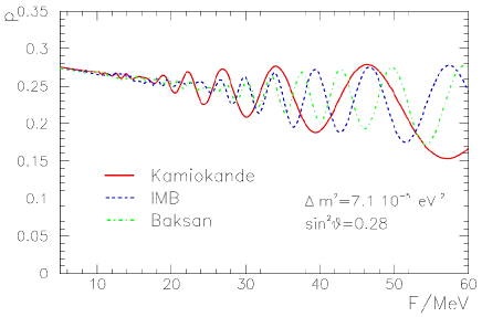
In [212], they took the spectrum parameterization in Eq. (136). Then, given the parameters $E_{0e},E_{0x},L_{e},L_{x},\beta_{e}$ and $\beta_{x}$, we can calculate the observed average energies and event numbers expected at Kamiokande II and IMB. Fig. 69 shows the average energy of positrons (left) and event numbers (right) at the Kamiokande II and IMB as functions of the average energy of the original $\bar{\nu}_{e}$, $E_{0\bar{e}}$, and different values of $E_{0x}/E_{0e}$ and $L_{x}/L_{e}$. Neutrino oscillation parameters are set to the same value as in Fig. 68.

Let us consider first the no-oscillation case. From the left of Fig. 69, we obtain the $\bar{\nu}_{e}$ average energy: from Kamiokande II data,

$$E_{0e}^{\rm K2}=8.7\pm 0.9{\rm MeV},$$ (223)

and from IMB data,

$$E_{0e}^{\rm IMB}=14.7\pm 1.9{\rm MeV}.$$ (224)

Thus, the IMB result is more than $3\sigma$ above the Kamiokande II result. According to the right of Fig. 69, the expected event numbers at Kamiokande II and IMB for the energies $E_{0e}^{\rm K2}$ and $E_{0e}^{\rm IMB}$ and $L_{e}=5.3\times 10^{52}{\rm erg}$ are $N_{e}^{\rm K2}=7.8\pm 1.5$ and $N_{e}^{\rm IMB}=10^{+6}_{-4}$, respectively. Therefore, to reproduce the observed event numbers at Kamiokande II and IMB,

$$L_{e}^{\rm K2}=8.2\times 10^{52}~{}{\rm erg},~{}~{}~{}L_{e}^{\rm IMB}=4.2\times 10^{52}~{}{\rm erg},$$ (225)

are required, respectively. Thus, the IMB signal implies about 2 times higher average energy and 2 times smaller luminosity in comparison with Kamiokande II.

Neutrino oscillation improves the agreement between the Kamiokande II and IMB. For $E_{0x}/E_{0e}=1.6$ and $L_{x}/L_{e}=1$, we obtain,

$$E_{0e}^{\rm K2}=6.8\pm 0.8~{}{\rm MeV},~{}~{}~{}E_{0e}^{\rm IMB}=10.3\pm 1.7~{}{\rm MeV},$$ (226)

which now agree in $2\sigma$ level. Actually, a ”concordance” model with

$$E_{0e}=8{\rm MeV},~{}~{}~{}E_{0x}=12.8{\rm MeV},$$

$$L_{e}=L_{x}=8\times 10^{52}{\rm erg},$$

$$\beta_{e}=\beta_{x}=4,$$ (227)

gives the best fit to the all available data with $\chi^{2}=11.0$ while the best-fit no-oscillation model with

$$E_{0e}=11{\rm MeV},~{}~{}~{}L_{e}=5.3\times 10^{52}{\rm erg},~{}~{}~{}\beta_{e}=4,$$ (228)

gives $\chi^{2}=16.2$. Thus neutrino oscillation leads to a certain improvement of the global fit of the data. The improvement requires lower average energy of the original $\bar{\nu}_{e}$ spectrum and larger $\bar{\nu}_{e}$ luminosity. The combination of smaller average energy and larger luminosity corresponds to a larger radius of the neutrinosphere: $R_{\rm ns}\propto E_{0e}^{-2}L_{e}^{1/2}$. It follows that in the concordance model $R_{\rm ns}$ is about 2.4 times larger than in the no-oscillation model, which gives $R_{\rm ns}=(20-30){\rm km}$ [206].

The concordance model gives rather small average energies of $\bar{\nu}_{e}$ and $\nu_{x}$ compared to those predicted by numerical simulations. The situation becomes even worse with adiabatic H-resonance, where most of the observed neutrinos were originally $\nu_{x}$s. Because $\nu_{x}$s are expected to have larger average energy than $\bar{\nu}_{e}$, $E_{0x}$ must be substantially smaller than that predicted by numerical simulations. Anyway, since the event numbers of SN1987A neutrinos would be too small to make a definitive conclusion. We are looking forward to seeing the next galactic supernova.

4.5 Neutrino detectors

It took 25 years to prove the existence of neutrinos experimentally since Pauli predicted theoretically in 1931. It took another 30 years to use neutrinos as tools in particle physics and astrophysics. This is because neutrinos have very weak interaction with other particles. Since the cross section of neutrino reaction is typically $10^{-40}{\rm cm}^{2}$, mean free path of neutrinos in water is about $10^{16}{\rm cm}$. This is why the current neutrino detectors are huge in volume. In this section we explain various neutrino detectors and their detection principles.

4.5.1 water, heavy water and ice

Neutrino interactions in water produces a relativistic charged particle which is mostly an electron or positron. If the velocity of the charged particle is larger than velocity of light in water, the charged particle emits Cherenkov light. This Cherenkov light is the signal of water Cherenkov detector. There are many neutrino detectors which utilize this method, starting from Kamiokande and IMB to the current experiment SuperKamiokande (SK), Sudbury Neutrino Observatory (SNO) and IceCube (AMANDA). They are based on the same detection strategy but have different features which come from different target media: SuperKamiokande, SNO and IceCube use pure water, heavy water and antarctic ice, respectively.

neutrino reactions in water

Cross sections of neutrino reactions in water at low energies, $s\leq m_{W}^{2}$, where $s$ is the center-of-mass energy and $m_{W}$ is the $W$ boson mass, are given by,

$$\sigma(\nu_{e}e\rightarrow\nu_{e}e) = 9.33\times 10^{-44}\left(\frac{E_{\nu}}{10{\rm MeV}}\right){\rm cm}^{2},$$ (229)

$$\sigma(\bar{\nu}_{e}e\rightarrow\bar{\nu}_{e}e) = 3.88\times 10^{-44}\left(\frac{E_{\nu}}{10{\rm MeV}}\right){\rm cm}^{2},$$ (230)

$$\sigma(\nu_{x}e\rightarrow\nu_{x}e) = 1.59\times 10^{-44}\left(\frac{E_{\nu}}{10{\rm MeV}}\right){\rm cm}^{2},$$ (231)

$$\sigma(\bar{\nu}_{x}e\rightarrow\bar{\nu}_{x}e) = 1.30\times 10^{-44}\left(\frac{E_{\nu}}{10{\rm MeV}}\right){\rm cm}^{2},$$ (232)

$$\sigma(\nu_{\mu}e\rightarrow\mu\nu_{e}(s\gg m_{\mu}^{2})) = 1\times 10^{-41}\left(\frac{E_{\nu}}{1{\rm GeV}}\right){\rm cm}^{2},$$ (233)

$$\sigma(\bar{\nu}_{e}p\rightarrow e^{+}n) = 9.77\times 10^{-42}\left(\frac{E_{\nu}}{10{\rm MeV}}\right)^{2}{\rm cm}^{2},$$ (234)

$$\sigma(\nu_{e}{}^{16}{\rm O}\rightarrow e^{-}{}^{16}{\rm F}) = 1.1\times 10^{-42}\left(\frac{E_{\nu}-13{\rm MeV}}{10{\rm MeV}}\right)^{2}{\rm cm}^{2},$$ (235)

$$\sigma(\bar{\nu}_{e}{}^{16}{\rm O}\rightarrow e^{-}{}^{16}{\rm N}) = 1.1\times 10^{-42}\left(\frac{E_{\nu}-13{\rm MeV}}{10{\rm MeV}}\right)^{2}{\rm cm}^{2},$$ (236)

and shown in Fig. 71.

Figure 70: Cross sections of neutrino interactions in water. The dominant interaction is $\bar{\nu}_{e}p\rightarrow e^{+}n$ at every energy.

Figure 71: Angular distribution of scatter electron in $\nu_{e}e^{-}\to\nu_{e}e^{-}$ with $E_{\nu_{e}}=5$ and 10 MeV.

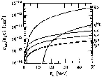
Among these, the inverse beta decay (234) has the largest cross section at all energies so that most of the events at water Cherenkov come from this reaction. Because the emitted positron has an almost isotropic distribution for low-energy neutrinos like supernova neutrinos, it is difficult to know the direction of the incident neutrino.

On the other hand, electron scattering event gives us information of the direction of the incident neutrino, although the cross section is much smaller than that of the inverse beta decay. The angle between the scattered electron and the incident neutrino is given by,

$$\cos{\theta}=\frac{E_{\nu}+m_{e}}{E_{\nu}}\left(\frac{1}{1+2m_{e}/E_{e}}\right)^{1/2},$$ (237)

where $m_{e}$ and $E_{e}$ are the electron mass and electron energy, respectively. Angular distribution of the scattered electron in $\nu_{e}e^{-}\to\nu_{e}e^{-}$ is plotted in Fig. 71. Here it should be noted that electron scattering occurs for all the flavors and they cannot be distinguished at low energies ($s\ll m_{\mu}$), although the cross sections are different. The $\nu_{e}e^{-}$ cross section is larger than those of the other flavors because electron scattering of $\nu_{e}$ is contributed from the charged current interaction as well as the neutral current interaction.

SuperKamiokande

The SuperKamiokande [306] detector is a cylindrical 50,000 ton water Cherenkov detector located at the Kamioka mine in Japan. It lies 1,000 m underneath the top of Mt. Ikenoyama, (i.e. 2,700 m water equivalent underground), resulting in a cosmic ray muon rate of 2.2 Hz, a reduction of 10.5 compared to the rate at the surface. As a supernova neutrino detector, SK has a fiducial volume of 32,000 ton.The detector is optically separated into two regions, the inner and outer detectors. The inner detector of the SuperKamiokande-I detector, which operated from April 1996 to July 2001, was instrumented with 11,146 50-cm diameter inward facing photomultiplier tubes (PMTs) which provide $40\%$ photocathode coverage. This photocathode coverage made it possible to detect low energy electrons down to $\sim 5$ MeV. Also, SK uses the anti-counter which surrounds the inner detector detect and remove events due to cosmic-ray muons. The direction of a charged particle is reconstructed using the directionality of the Cherenkov light. Angular resolution is about 25 degree for a 10 MeV electron. Energy resolution $\sigma$ for low-energy neutrinos is given by,

$$\sigma=1.5\left(\frac{E}{10{\rm MeV}}\right)^{\frac{1}{2}}{\rm MeV}.$$ (238)

As discussed in section 3.4, SK has been playing a central role in the field of neutrino oscillation experiment by observing neutrinos from the sun, atmosphere and accelerator. It is also expected to give tremendous information on supernova if it occurs in the future. For a detailed description of SK detector, see [309].

Due to an unfortunate accident in 2001, $60\%$ of the PMTs were destroyed and the observation was interrupted for a while. However, the observation was restarted by redistributing the survived PMTs and SK is expected to resume normal observation with the original number of PMTs in 2006.

IceCube

IceCube [147] is an extended experiment of AMANDA [6, 7] and consists of an array of 4800 optical modules on 80 strings, regularly spaced by 125 m in antarctic ${\rm km}^{3}$ ice. It covers an area of approximately $1{\rm km}^{2}$, with the optical modules at depths of 1.4 to 2.4 km below surface. Each string carries 60 optical modules, vertically spaced by 17 m. IceCube is primarily designed to observe high-energy neutrinos ($E>1{\rm TeV}$) from astrophysical sources. In order to reach the large volume needed to detect the expected small fluxes at high energies, the density of optical modules must be too sparse to measure low-energy neutrinos such as solar neutrinos. However, it is expected that IceCube can detect a supernova neutrino burst because the Cherenkov glow of the ice can be identified as time-correlated noise among all phototubes. The observed quantity is the number of Cherenkov photons caused by supernova neutrinos as a function of time. Thus, although IceCube cannot identify individual neutrino, it can measure neutrino luminosity of supernova. For a detailed description of IceCube, see [148]. Supernova neutrino detection at IceCube was studied in detail in [116, 76].

Sudbury Neutrino Observatory

Figure 72: Cross sections of neutrino interactions with deuteron. Solid lines are neutrinos and dashed lines are antineutrinos.

Sudbury Neutrino Observatory (SNO) [293] is located in a large cavity excavated at the 2,039 m level (6,000 m water equivalent) in the Creighton mine near Sudbury. The 1,000 tons of heavy water are contained in an acrylic vessel surrounded by a light water shield.

SNO’s uniqueness is the use of heavy water as its neutrino detection medium. Neutrinos interact in heavy water in two additional ways not possible in ordinary water. One is through the charged current interaction:

$$\nu_{e}+d \rightarrow e^{-}+p+p~{}(E_{\rm th}=1.44{\rm MeV}),$$ (239)

$$\bar{\nu}_{e}+d \rightarrow e^{+}+n+n~{}(E_{\rm th}=4.03{\rm MeV}),$$ (240)

whose cross sections are plotted in Fig. 72. These neutrino absorption reactions can only happen if the neutrino is an electron neutrino or electron anti-neutrino at low-energies ($s<m_{\mu}^{2}$). Thus the neutrino absorption reaction exclusively counts electron neutrinos and electron anti-neutrinos.

Another is the deuteron breakup reaction:

$$\nu+d\rightarrow\nu+n+p~{}(E_{\rm th}=2.22{\rm MeV}).$$ (241)

This reaction occurs through the neutral current interaction and it occurs with equal probability for all neutrino flavors. In this reaction, no new charged particle is created and the free neutron cannot by itself create Cerenkov light. However, after scattering off of the nuclei in the heavy water it is eventually captured by another deuteron, creating a tritium nucleus and releasing a high energy $\gamma$ ray. This $\gamma$ ray then scatters an electron in the heavy water and it is this secondary electron which creates the Cerenkov light.

SNO played a critical role in solving the solar neutrino problem with its ability to identify $\nu_{e}$ and neutral current events, as discussed in section 3.4.5. This feature will also have a great impact on observation of supernova neutrinos. For a detailed description of SNO, see [294].

4.5.2 scintillator

As a high energy particle propagates in medium, it loses energy exciting electrons in the medium. A part of the deposited energy is emitted as scintillation photons. Scintillator detector uses the scintillation photons as a signal to detect high energy particles. Here we summarize basic feature of scintillator detector as a neutrino detector.

As to neutrino detector, liquid hydrocarbon is often used as a medium. In this medium, neutrinos interact with electrons, protons and carbon nuclei. Dominant contribution to the events comes from inverse beta decay,

$$\bar{\nu}_{e}+p\rightarrow e^{+}+n,$$ (242)

where the positron has almost the same energy as that of the incident neutrino. Then the neutron is absorbed into proton in about $170\mu{\rm sec}$,

$$n+p\rightarrow d+\gamma_{2.2{\rm MeV}}~{}~{}~{}(E_{\rm th}=1.80{\rm MeV}),$$ (243)

and the emitted photon scatter an electron, which then emits Cherenkov photons. Thus the positron and the delayed 2.2 MeV photon are the signal of inverse beta decay.

Since carbon nuclei are abundant in scintillator, the following reactions also contribute to the events,

1. neutral current interaction

   $${}^{12}{\rm C}+\nu\rightarrow{}^{12}{\rm C}^{*}+\nu\;\;(E_{\rm th}=15.11{\rm MeV}),$$ (244)

   $${}^{12}{\rm C}^{*}\rightarrow{}^{12}{\rm C}+\gamma_{15.11{\rm MeV}},$$ (245)

2. $\nu_{e}$ capture by charged current interaction

   $${}^{12}{\rm C}+\nu_{e}\rightarrow{}^{12}{\rm N}+e^{-}~{}~{}(E_{\rm th}=17.34{\rm MeV}),$$ (246)

   $${}^{12}{\rm N}\rightarrow{}^{12}{\rm C}+e^{+}+\nu_{e}~{}~{}(\tau_{1/2}=11.00{\rm msec}),$$ (247)

3. $\bar{\nu}_{e}$ capture by charged current interaction

   $${}^{12}{\rm C}+\bar{\nu}_{e}\rightarrow{}^{12}{\rm B}+e^{+}~{}~{}(E_{\rm th}=14.39{\rm MeV}),$$ (248)

   $${}^{12}{\rm B}\rightarrow{}^{12}{\rm C}+e^{+}+\nu_{e}~{}~{}(\tau_{1/2}=20.20{\rm msec}).$$ (249)

The cross section of these reactions are plotted in Fig. 73. Because each reaction has its unique signal, we can identify them including inverse beta decay. This is an advantage of scintillator detector.

Figure 73: Cross sections of neutrino interactions with ${}^{12}{\rm C}$. Solid lines are neutrinos and dashed lines are antineutrinos.

KamLAND

KamLAND (Kamioka Liquid scintillator Anti-Neutrino Detector) is located underneath Mt. Ikenoyama in Gifu prefecture in central Japan, where Kamiokande was once located. It is a 1,000 ton liquid scintillator which is composed of $80\%$ dodecane and $20\%$ pseudocumene, whose typical composition is ${\rm C}_{n}{\rm H}_{2n}$. The primary purpose of the KamLAND is to probe the LMA solution of the solar neutrino problem by observing reactor neutrinos from the entire Japanese nuclear power industry as discussed in section 3.4.3.

Because of low background level, KamLAND is also suitable for observation of supernova neutrinos. In [28], supernova neutrino detection at KamLAND was studied.

LVD

LVD (Large Volume Detector) is located in the INFN Gran Sasso National Laboratory, Italy. It consists of an array of 840 liquid scintillator (${\rm C}_{n}{\rm H}_{2n+2}$ with $\langle n\rangle=9.6$) counters and the active scintillator mass is 1,000 ton. The main purpose of the project is detection of supernova neutrinos. For details of the detector, see [2, 283]. Analyses of supernova neutrinos expected to be observed at LVD were performed in [210, 320].

5 Explosion Mechanism of Core-Collapse Supernovae

5.1 Status of Spherical Models

Although the gross physical conditions of core-collapse supernovae are understood as denoted in the section 2, recent numerical simulations assuming spherical symmetry, however, with the current input physics (neutrino interactions and the equations of state of dense matter) and with/without general relativity, do not yield successful explosions by the neutrino heating mechanism (see Figure 74) [264, 198, 331, 201].

The problem apparently stems from the weak-interacting natures of neutrinos. The neutrino heating occurs only inefficient for the successful explosions in the spherical models. Whether neutrinos succeed in reviving the stalled shock wave depends on the efficiency of the energy transfer to the postshock layer, which in turn increases with the neutrino luminosity. In fact, it was pointed out that the stalled shock revives leading to explosions for otherwise failed explosion models by enhancing the neutrino luminosity artificially by a few tens percents from the original value [155] (see Figure 75 and compare 1D/2.10 and 1D/2.225). It was also found by the study of the static configurations after the shock-stagnation that for a given accretion rate there is a critical luminosity for the shock revival [49] (see Figure 76).

Figure 74: Comparison of the radial position of the shock waves as a function of time obtained by the two independent groups. The thin and thick lines are based on the simulations of a $15M{\odot}$ progenitor star, performed by vertex code of the Garching group [264] and agile-boltztran code of Oak Ridge-Basel group [199], respectively. It is shown that spherically symmetric models with standard microphysical input fail to explode by the delayed, neutrino-driven mechanism. This figure is taken from Liebendörfer et al [201].

Figure 75: Shock positions as a function of time after core bounce taken from [155]. 1D or 2D represents the one or two dimensional models. The numbers indicate the size of the neutrino luminosities in unit of $10^{52}~{}\rm{erg}~{}\rm{s}^{-1}$ injected from the proto-neutron star. Given a neutrino luminosity of $2.1\times 10^{52}~{}\rm{erg}~{}\rm{s^{-1}}$, it can be seen that the unsuccessful explosion model in the 1D simulation turns to lead the successful explosion in the 2D simulation. Generally, the shock can propagate to the outer regions in the 2D simulations due to the convection in the hot bubble, which boosts the neutrino-heating efficiency.

Figure 76: Critical curve for the shock-revival as a function of the neutrino luminosity ($L_{\nu_{e}}$ in unit of $10^{52}~{}{\rm erg}~{}{\rm s}^{-1}$) emitting from the central protoneutron star and the accretion rate ($\dot{M}$ in unit of $M_{\odot}$) through the stalled shock. The “Model Trajectory” in this figure is taken from the results obtained in the numerical simulations by Bruenn (1982) [58], in which no explosion was obtained. If the evolution line of a real core crosses the critical curve into the hatched region, a neutrino-driven supernova should begin. This figure is taken from Burrows & Goshy (1993) [49].

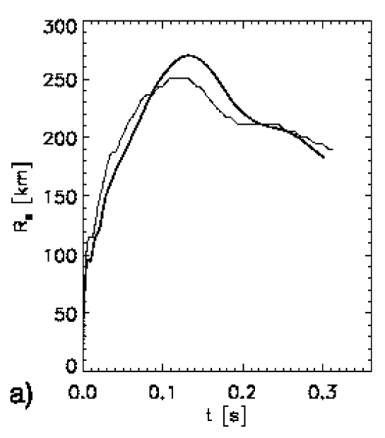
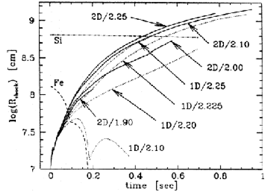
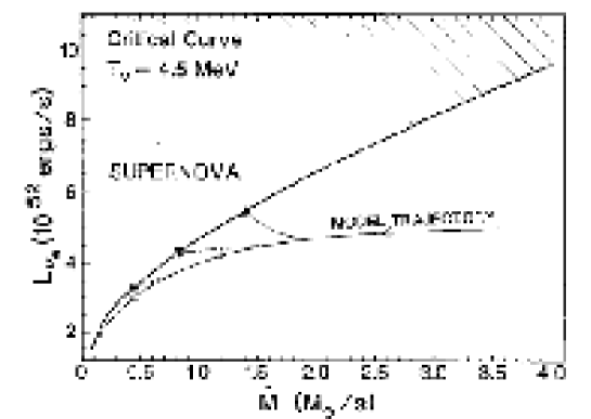
Janka et al. reported that the manipulation of omitting the velocity dependent term ($O(v/c)\sim 10\%$) in the neutrino transport equations increased the neutrino energy deposition in the heating region and was sufficient to covert a failed model into a exploding one [156]. These facts suggest that all we have to obtain for the successful explosions, is the relatively small amount of boost of the neutrino luminosity and energy from the values we have obtained in the failed explosion models.

In the last couple of years, both numerics and microphysics have been developed. The former, in particular, has seen major progress [264, 198, 331, 201, 45]. Ever since Wilson first proposed the neutrino heating mechanism [358], the accurate treatment of neutrino transport has been an important task, however mainly due to the computational intensity, some approximations, such as the multi-group-flux-limited diffusion approximation as the most familiar example [55, 56, 234], have been employed in the 1D spherical symmetric simulations. This situation has changed completely lately (see [61] for a complete set of references). A couple of groups [264, 198, 331, 201], have published the state-of-the-art direct solutions of the Boltzmann equation for neutrinos, some of them extended even to 2D computations in the multi-group-flux-limited diffusion approximation [45, 202]. Although they have still not found successful explosions, the importance of the accurate treatment of neutrino transfer should be never missed.

The microphysics such as neutrino reaction rates and equations of state have also been studied in detail. Recently, shell-model calculations of nuclear properties [191] revealed that the treatment of the electron capture rates for various nuclei should be changed significantly from the previous ones [55]. In almost all the supernova simulations, the electron captures rates on nuclei were cut off above a few $\sim 10^{10}~{}{\rm g}~{}{\rm cm}^{-3}$ because only the resonant Gamow-Taylor transitions could be treated in the average heavy nuclei, which is calculated by the employed equation of state (EOS) [55].

Figure 77: The electron fraction, entropy, density and velocity as functions of the enclosed mass at the beginning of bounce for a 15 $M_{\odot}$ model. The thin line is a simulation using the conventional capture rates by Bruenn parametrization [55] while the thick line for a simulation using the new rates by Langanke Martínez-Pinedo (LMP) [189, 190]. This figure is taken from Hix et al. (2003) [136].

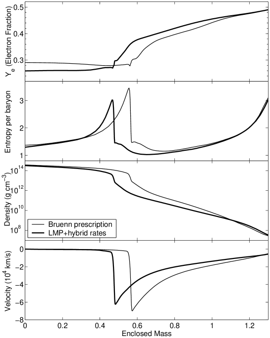
Despite of the quantitative change of the electron capture rates and hence the lepton fraction at the central portion of the core, subsequent shock propagations were found to show no significant change in comparison with the previous studies due to cancellation effects [136] (see Figure 77).

As for the EOS of dense matter, we have at least two kinds of EOS now available based on different realistic descriptions of nuclear interactions, namely EOS by Lattimer & Swesty (LS EOS) [187] and EOS by Shen et al (SHEN EOS) [287]. Sumiyoshi et al. performed 1D adiabatic hydrodynamic simulations employing the two kinds of equations of state, respectively, and found that there does appear the difference in the chemical compositions between the EOS’s during the infalling phase, however, which disappears in the later phases, and hence no significant differences such in the remnant masses and the explosion energies are obtained [303]. Currently they performed the general relativistic neutrino radiation hydrodynamic core-collapse simulations assuming spherically symmetric and investigated long-term postbounce evolution after core-bounce employing the two equations of state. They found that, for both EOSs, the core does not explode and the shock waves stall similarly in the first 100 milliseconds after core bounce (see Figure 78).

Figure 78: Radial positions of shock waves in models employing SHEN EOS and Lattimer & Swesty EOS are shown by thick and thin lines, respectively, as a function of time after bounce. The evolutions at early and late times are displayed in left and right panels, respectively. This figure is taken from Sumiyoshi et al (2005) [304].

As for the neutrino reaction rates, the effects of the inter-nucleon many body effects near nuclear density have been elaborately studied (see Figure 79 and [52, 53, 267, 369].) Inter-ion correlations work for suppressing the neutrino-nucleus elastic scattering [141, 149], however, have been pointed out to lead to non noticeable changes of the dynamic during core-collapse (see Figure 80, [60, 223]). Relatively small corrections to the standard neutrino interaction processes [55] such as the detailed reaction kinematics of nucleon thermal motions, recoil, and weak magnetism contributions [142] as well as nucleon bremsstrahlung ($NN^{{}^{\prime}}\rightleftharpoons NN^{{}^{\prime}}\nu\bar{\nu}$) [118], pair-annihilation/creations among different neutrino flavors [46], such as $\nu_{e}+\bar{\nu}_{e}\rightarrow\nu_{\mu,\tau}+\bar{\nu}_{\mu,\tau}$ (see Figure 81), and the quenching of the axial vector coupling constants in dense matter [62] have been partly or fully incorporated and their importance has been evaluated in the recent 1D computations [266, 331, 45]. These nuclear corrections effectively work for the suppression of the opacities leading to the larger neutrino luminosities, which is able to act in favor of enhancing the explosion [266].

Figure 79: Effect of inter-nucleon interactions on the neutrino-nucleon scattering rates taken from [369]. Left and right panels show the contours of the suppression and enhancement factors, which is the ratio of the scattering rate with to without the corrections. The top and bottom panel shows the contribution from the density correlation function ($R_{1}$, vector currents) and the spin-density correlation ($R_{2}$, axial-vector currents), respectively. Note the difference of the density scale in the right and left panels. It can be seen that the scattering rate is suppressed due to the corrections in the high density regime ($\rho\geq 10^{14}~{}{\rm g}~{}{\rm cm}^{-3}$) (see left panels), while the vector current contribution (right top panel) is enhanced in the low density region ($\rho\leq 10^{14}~{}{\rm g}~{}{\rm cm}^{-3}$) and in the vicinity of the liquid-gas phase transition regions (the dark regions in the right panels). The above features are generally common in case of the other values of the proton fraction, $Y_{\rm p}$. See for details Yamada and Toki (2000) [369].

Figure 80: Effect of ion-ion correlations on neutrino-nucleus elastic scattering during core-collapse of a $25M_{\odot}$ progenitor star taken from [60]. Left panel shows the optical depth along a radial path from the stellar center to the surface of as a function of the neutrino energy when the central density is $10^{14}~{}{\rm g}~{}{\rm cm}^{-3}$. Right panel shows the lepton fraction profiles at the same time with the right panel. From the left panel, the optical depth of the lower-energy neutrinos is shown to be lowered due to the screening effect of nucleus (compare the lines labeled as A and B). On the other hand, this change leads to a smaller change of the lepton fraction $\sim 0.015$ in the central region (right panel).

Figure 81: The pair-production rates by the process $\nu_{e}+{\bar{\nu}}_{e}\rightarrow\nu_{\mu,\tau}+\bar{\nu}_{\mu,\tau}$ (top line) and $e^{+}+e^{-}\rightarrow\nu_{\mu,\tau}+\bar{\nu}_{\mu,\tau}$ (bottom line) as a function of the degeneracy parameter of electron-type neutrinos ($\eta_{\nu_{e}}$) and of electrons ($\eta_{e}$), respectively. Here $T=12$ MeV and $\eta_{\nu_{\mu,\tau}}=0$ is assumed. The new rate, namely, $\nu_{e}+{\bar{\nu}}_{e}\rightarrow\nu_{\mu,\tau}+\bar{\nu}_{\mu,\tau}$, is shown to dominate over the electron-positron pair reaction, which was considered only the sources for producing $\nu_{\mu,\tau}$ and $\bar{\nu}_{\mu,\tau}$. This figure is taken from Buras et al. (2003) [46].

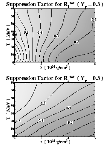
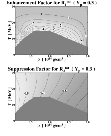
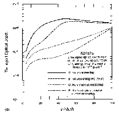
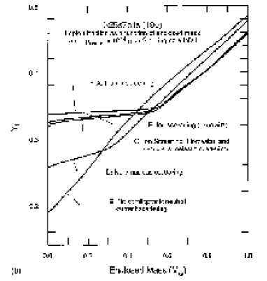
However even with these sophistications, the successful explosion has not yet been found for the present [266, 45]. We may still missing some important microphysical processes if we are to obtain the successful explosion assuming spherical symmetry. The phase transitions with various possible geometrical structures from isolated nuclei to uniform nuclear matter (the so-called “nuclear pasta”) have been elaborately studied from a nuclear physics point of view [346, 347]. Due to this non-uniformity of the nuclei, the neutrino opacities are shown to be lowered, which are conventionally estimated by a single heavy nucleus approximation [144]. The inelastic neutrino-nucleus interaction has been pointed out to play the same important role of thermalizing neutrinos as effective as the neutrino scattering on electrons [57]. These microphysical ingredients, which have not been routinely taken into the modern supernova simulations, should deserve further investigations.

5.2 Multidimensional Aspects in Core-Collapse Supernovae

Ever since SN1987A was observed, most researchers in this field think that the dynamics of supernova is aspherical. The following observations of SN1987A have been attainable because SN 1987A is the nearest supernova for us and thus have been observed by modern observational instruments. For the explanation of the observed shape of the lightcurve, the unexpectedly early appearance of X, $\gamma$-ray emissions, and Doppler features of spectral lines, the existence of a large-scale mixing between the deep interior and the hydrogen envelope is suggested (for a recent review, see [252]). The expanding debris of SN1987A is directly confirmed to be globally asymmetric by images of Hubble Space Telescope (HST) [261] and its axis roughly aligns with the small axis of the rings [345] (see the left panel of Figure 82). In recent years, it is noted that the same features are drawn for other core-collapse supernovae (see [138] and references therein). Spectroporalimetry shows that substantial asymmetry is common in core-collapse supernovae, indicating bi-polar explosions with axis ratios up to $\sim 2$ [345, 244, 137, 343, 344]. The degree of the asymmetry tends to increase with time when greater depths are observed [344, 203]. Both suggests that a connection of the asymmetries with the central engine. For core-collapse supernovae with good time and wavelength coverage, the orientation of the polarization vector tends to stray constant both in time and with wavelength, which suggest that there is a global symmetry axis in the ejecta [344, 203]. Two oppositely directed jets [107] with the ejected material in a toroidal structure [351] around the center have been observed in the remnant of Cas A supernova. Young neutron stars are observed with high space velocities (typically $300-400$ km/s [213, 204], with highest values greater than $1000$ km/s [17]), which are most likely imparted to the neutron star by a kick at the moment of the explosion. Interestingly, the recent X-ray observations have shown the correlation between the direction of pulsar motions and the spin axis of their supernovae in Vela and Crab pulsars [127, 260] (see the middle and right panels of Figure 82). All these observational evidences can be naturally interpreted as an evidence that the inner portions of the explosion are strongly aspherical.

Figure 82: Observational evidences for asphericity in core-collapse supernovae. Left panel shows the inner debris of the supernova ejecta with an axis ratio of $\sim$ 2 (inner red region) and the ring around it produced in the presupernova era (taken from [345]). The middle and right panel shows the nebulae of Vela and Crab pulsars, respectively (taken from [260] and [349]).

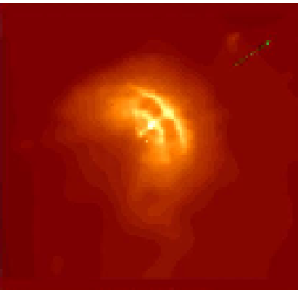
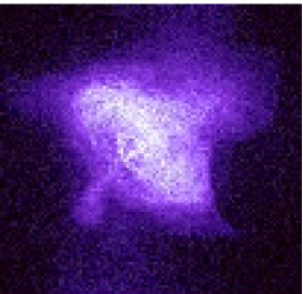
So far many physical ingredients have been suggested in order to produce such asymmetric explosions. We review each ingredient one by one in the following.

5.3 Roles of Convections and Hydrodynamical Instabilities

The convections and hydrodynamical instabilities have been long supposed to be responsible for producing the aspherical explosions. We give a summary of past studies about them, paying attention to where and why the convections and instabilities are likely to occur in the supernova cores and their possible roles of producing the aspherical explosions.

5.3.1 convection near and below the protoneutron star

It has been widely recognized that the convection in the protoneutron star (PNS) could play a crucial role in enhancing the neutrino luminosities from the PNS. In fact, Wilson and his collaborators obtained the exploding models [359, 360], in which a neutron-finger convection, which will be stated below, in a PNS was assumed, otherwise they did not see the successful explosions. This illuminates the importance of the convection in the PNS.

After the shock wave stalls ($t\sim 10~{}{\rm ms}$ after core bounce), the outer parts of the PNS are convective unstable, because the deleptonization occurring in the shocked material outside the neutrino sphere produces a negative lepton gradient and the weakening of the prompt shock wave gives rise to a negative entropy gradient in the same region. Epstein first proposed that these two factors are an sufficient condition for the so-called prompt convections to occur [86]. In fact, the existence of these instabilities were demonstrated in most hydrodynamic simulations ([48, 50] see, however, [59]).

After this prompt convection, the so-called “Neutron finger” instability develops inside the PNS [360]. This instability is driven in the presence of a positive entropy gradient and a negative lepton gradient, both of which are mostly satisfied inside the PNS. In the long-run 2D hydrodynamical simulations in the PNS, Keil et al. found that the neutrino luminosities increase $\sim 50\%$ due to the convection at times later than $200-300$ ms after core bounce (see Figure 83), which are expected to crucial for reviving the stalled shock wave [172].

Figure 83: Convection inside the protoneutron star. Top left and right panels show the absolute values of the velocity for two instants (about 0.5s (left) and 1 s (right) obtained in the 2D simulations of [172]. The growth of the convective region can be seen. Bottom panel shows the time evolutions of neutrino luminosities $L_{\nu}$ and mean energies of $\nu_{e}$ and $\bar{\nu_{e}}$ for the model in the top panels without (“1D”; dotted) and with convection (“2D”: solid). Significant rise in the neutrino luminosities and energies can be clearly seen. Top panels are taken from Janka and Keil [151], and the bottom panel is taken from Keil et al [172].

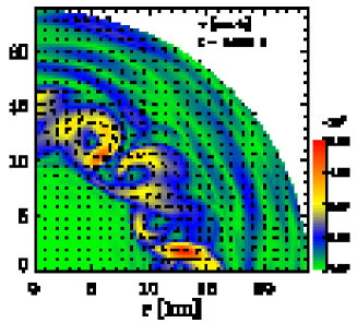
It is noted that their neutrino transport was coupled only to the radial directions and thus suppresses the neutrino transport in the angular directions, essentially underestimating the stabilizing effect of the neutrino transport. On the other hand, Mezzacappa et al found only mild convective activity in the region near the neutrino sphere [235]. Since the neutrino transport in Mezzacappa et al [235] was assumed to be spherical, it might result in overestimating the stabilizing effect [235] (see Figure 84). The recent two-dimensional numerical simulation shows that the PNS convection really does occur, however, is not important for boosting the neutrino luminosity, because the convectively active layer is formed rather deep inside the PNS and is surrounded by a convectively stable shell [45]. However, one may argue that the conclusion may be still subject to change because their neutrino transport, albeit in the state-of-the-art manner, is not fully spatially two-dimensional, and hence could not reproduce all of the properties of the convective flows.

Figure 84: Two-dimensional plots showing the entropy distribution of the 15 $M_{\odot}$ model in a simulation “without” neutrino transport (top panel) and with neutrino transport (down panel). Taken into account the neutrino transport, albeit assuming spherical symmetry, it is seen that the instability in the protoneutron star is damped out within a short time. This figure is taken from Mezzacappa et al (1998) [235].

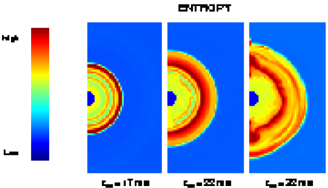
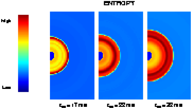
5.3.2 convection in the hot-bubble regions

In the hot bubble, in which the neutrino heating dominates over the neutrino cooling (the regions between $R_{g}$ and $R_{s}$ in Figure 8), convections are expected to occur by the negative entropy gradient. In fact, a dynamical overturn between the hot, neutrino-heated, rising materials above gain radius and the cold postshock matter beneath has been demonstrated in the two-dimensional [128, 129, 50, 155, 269] or the three-dimensional [99] numerical simulations. As clearly demonstrated in [155], these convections indeed aid the shock revival and can lead to explosions in the case where the spherical models fail.

In most of the preceding studies, it is noted that the neutrino luminosities from the protoneutron star are given by hand at some inner boundary (the so-called lightbulb approximation). In order to boost the neutrino-heating efficiency by the convection in the hot bubbles, a sufficient deposition of the neutrino luminosity from the hot protoneutron star is required, which unfortunately no previously published models with the neutrino transport in the whole regions have failed to reproduce.

Figure 85: Left panel shows the time evolution of the gas entropy (from left to right in this panel), illustrating the growth of the instability induced by the aspherical perturbation, which is added at the stalled shock initially. Right panel shows the time evolution of the two-dimension simulation of the left panel in spacetime diagrams. The color at a given radius and time corresponds to the angle-average of the absolute value of the tangential velocity (right top) and absolute value of the deviation of pressure from the steady-state solution, $\Delta P/P$ (right bottom). The downflow of the tangential velocity is seen to be reflected at the inner boundary, producing the pressure perturbation propagating outwards (see the stripes in the top and down panels). Direct evidence of the vorticity-acoustic cycle are seen in these velocity plots. These figures are taken from Blondin et al [38].

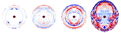
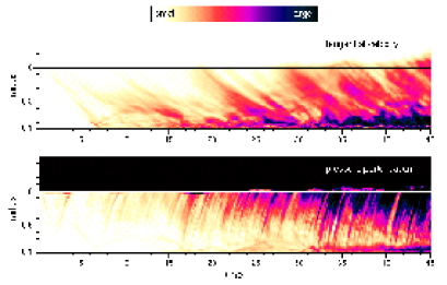
5.3.3 instability induced by the non-radial oscillation of the stalled shock waves

It is recently pointed out that the stalled shock waves are subject to low-mode ($l=1~{}{\rm or}~{}2$) aspherical oscillations [38]. Interestingly, it is not due to the convection induced by the negative gradients of entropy or lepton fraction but due to the so-called vorticity-acoustic cycle. In the cycle, the vorticity perturbations given at the stalled shocks propagate inwards and reflected at some inner boundary, which is presumably the surface of the protoneutron star, producing the acoustic waves, and propagate outwards and create new vorticity perturbations when reaching the stalled shock waves. This closed cycle amplifies the growth of the aspherical oscillations (see Figure 85). This cycle was first discovered in the context of stability analysis of the accretion disk around the black holes [94, 95]. In the simulations by Blondin et al. [38], the oblique shock waves are found to feed vorticity in the postshock region and lead to growing turbulence. Although the model computations by them are not so realistic in the sense that no neutrino transport was included, which should affect the growth of the pressure waves predominantly by neutrino cooling, such instability seemingly appears in some recent realistic supernova simulations [157]. Combined with the convections and the hydrodynamical instabilities stated above, it is expected to have a good chance to obtain a successful explosion, because the neutrino heating mechanism seems very close to explosion as it is in the spherical collapse. However, the difficulties of multi-dimensional treatment of neutrino transport have hampered the definitive answer to this problem.

Although some smoothed particle hydrodynamic (SPH) simulations have found explosions induced by the combination of neutrino heating and convection in the heating region [129, 99], there has been persistent concern with their approximate treatment of neutrino transfer. This situation may be changing recently. Some groups are preparing for full spatially multi-dimensional neutrino transport simulations [45, 202]. In these simulations, the dynamics of the whole core is computed with a code implemented with a Boltzmann solver. But still no successful explosions have been reported so far. We may have to look for alternatives to the convections and the hydrodynamical instabilities in order to get the successful explosions.

5.4 Roles of Rotation

Figure 86: Initial angular velocity as a function of the radius obtained in the recent stellar evolution calculations [120, 121]. 15 (blue) and 20 (green) indicate the mass of the progenitor in unit of the solar mass ($M_{\odot}$). Much smaller angular velocities by models m15b4 and m20b4 were evolved taking into account of the magnetic fields. The dotted red lines were constructed with the rotation law of Eq. (250) using the central angular velocity $\Omega_{0}$ of E15 ($4~{}\rm{rad}~{}{s}^{-1}$). Labeled number in the dotted red lines, such as 100, 500, represents the values of $R_{0}$ in Eq. (250). This figure is taken from [258].

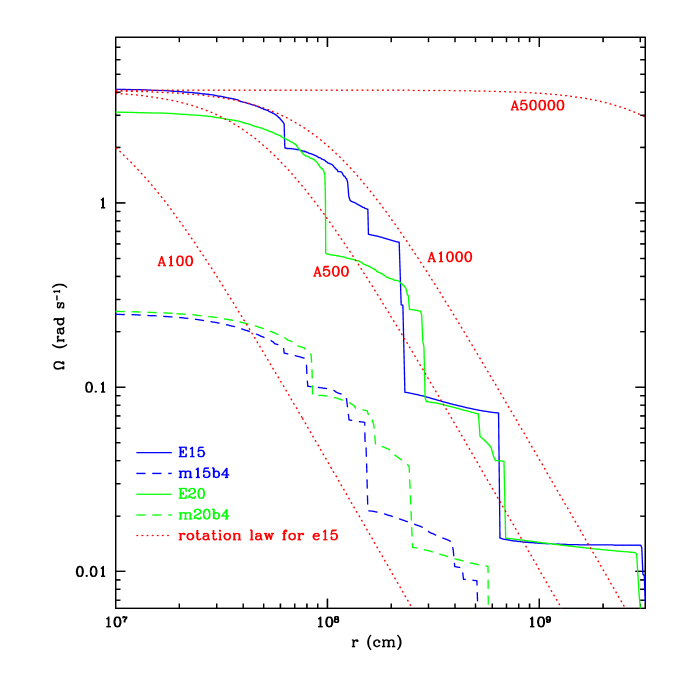
In addition to the hydrodynamical instabilities, rotation can produce the large asphericity in the supernova cores. It is well known that the progenitors of core-collapse supernovae are a rapid rotator on the main sequence [327]. Typical rotational velocity on the equator are on the order of $200$ km/s, which is the significant fraction of their breakup rotational velocity [108]. Recent theoretical studies suggest a fast rotating core prior to the collapse [120], although this is not conclusive at all when the magnetic fields are taken into account [121, 122] (see Figure 86). Neutron stars, which are created in the aftermath of the gravitational core collapse of massive stars at the end of their lives, receive the rapid rotation, which are believed to be observed as pulsars. From the above facts, rotation seems naturally to be taken into account in order not only to clarify the explosion mechanism, but also to explain the observed properties of core-collapse supernovae.

So far there have been some works devoted to the understanding of the effect of rotation upon the supernova explosion mechanism [239, 43, 274, 236, 366, 100, 101]. Among the studies, the systematic study of the rotational core-collapse, changing the initial angular momentum distributions and the strength has been done (see, for example, [366, 175, 258]). In the following, we show how the hydrodynamics in rotational core-collapse deviates from the one in spherical symmetry (section 2.3).

5.4.1 hydrodynamics in rotational core-collapse

The story of rotating core is not greatly different from the standard picture from the core bounce to the explosion as stated in section 2. In addition to the gravity and pressure gradients, one has to take into account the effect of centrifugal forces.

Figure 87: Time evolution of the shock wave near core bounce for a typical rotational core-collapse model (we call it model A), whose initial angular momentum distribution is based on the rotational progenitor model by [120]. The two snapshots show color-coded maps of entropy ($\rm{k_{B}}$) per nucleon together with the velocity fields. The left panel is for 2 msec after the core bounce when the shock wave begins to move upwards at the pole, the right panel is for 4 msec. In the case of weak differential rotation, it is found that the hot entropy blob is formed near the rotational axis and it moves upwards. Note the difference of the scale of the plots. These figures are taken from [175].

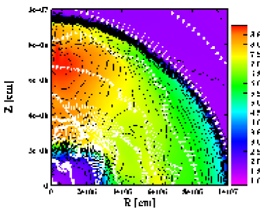
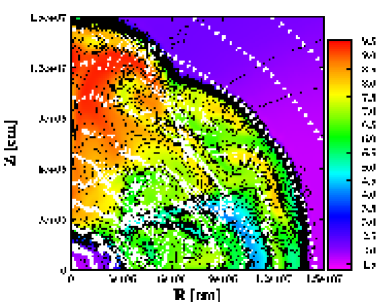
In Figure 87, the time evolution of the shock wave in a rotational core-collapse simulation [175] is shown. The initial angular velocity profile of this model is based on the rotational progenitor model by [120], which is approximately fitted by the following way,

$$\Omega(r)=\Omega_{0}\times\frac{{R_{0}}^{2}}{r^{2}+R_{0}^{2}},$$ (250)

where $\Omega(r)$ is an angular velocity, $r$ is a radius, and $\Omega_{0},R_{0}$ are model constants taking $\Omega_{0}=4~{}{\rm rad}~{}{\rm s}^{-1}$ and $R_{0}=1000~{}{\rm km}$ (see Figure 86 and A1000). As a sideremark we note that $r$ can be also interpreted as the distance from the rotational axis (the so-called cylindrical rotation). At first glance, the rotation profile seems more natural due to the Poincaré and Wavre theorem [327], however, the shellular rotation profile, in which the angular velocity is constant with radius, is also pointed out to be natural because the horizontal turbulence is likely to be much stronger than the vertical one during stellar evolutions with rotation (for an elaborate description of the presupernova models including rotation, the reader is referred to [126]). Since even the-state-of-the art rotational progenitor models are based on the spherically symmetric models, it may not be decided yet which rotation profile is correct. Considering the uncertainties of the progenitor models, the rotating pre-collapse models so far have been made by changing parametrically not only the rotational profile (shellular or cylindrical), but also the rotational velocity and the degree of the differential rotation, and then adding them to the spherically symmetric progenitor models.

Now let us return to the discuss of the model in Figure 87 again. At the central density of $2.3\cdot 10^{14}\rm{g}\,\,\rm{cm}^{-3}$, the model bounces at the pole first. The bounce epoch is slowed down of the order of $10{\rm~{}msec}$ than the one in absence of rotation due to the centrifugal forces acting against the gravitational pull. The occurrence of core bounce below the nuclear density ($\sim 3.0\times 10^{14}\rm{g}\,\,\rm{cm}^{-3}$) is a general feature in case of rotational core-collapse. This can be understood from the fact that rotation acts like a gas with an adiabatic index of $\gamma=5/3$. (see, for example, [327, 236, 271]) Due to this additional pressure support, whose gradient is steepest along the rotational axis, the core bounce occurs at the subnuclear density at the pole first.

After core bounce, the shock wave begins to propagate a little bit faster along the rotational axis supported by the buoyancy of the hot entropy blob ($S\geq 9.5\rm{k_{\rm B}}/\rm{nucleon}$) (see Figure 87). At this time $R$, which is the aspect ratio of the shock front, is 1.1, which is lowered to 1.0 by the shock stagnation (see the right panel of Figure 88). The initially prolate configuration ($R$ = 1.1) is stretched in the direction of the equator after the shock is weakened at the pole by the neutrino energy loss and ram pressure of the infalling material and finally stalls in the iron core. Note that a large angular momentum tends to push the matter parallel to the equatorial plane.

Depending on the total angular momentum and its distribution imposed initially on the iron core, the effects of rotation on the core dynamics have many variety. In Figure 88, the entropy distributions at the shock-stall for some representative models [175] are presented. In fact, a variety of the final profiles is immediately seen in the figure. As the initial rotation rate becomes larger, the shape of the stalled shock wave becomes more oblate due to the stronger centrifugal force (compare the left with right panel in Figure 88). If the initial rotation rate is the same, the shape of the stalled shock is found to be elongated in the direction of the rotational axis as the differential rotation becomes stronger (compare the left with the central panel of Figure 88). This is related with the production of high entropy blobs by core bounce. As mentioned above, the entropy blob formed near the rotational axis floats up parallel to the axis and then stalls for weak differential rotations. This makes the shock prolate at first. Then the matter distribution returns to be spherical or oblate due to the centrifugal forces. On the other hand, in the case of strong differential rotations, the shock wave formed first near the rotational axis hardly propagates and stalls very quickly. The high entropy blob begins to grow near the equatorial plane in this case. This then induces the flows towards the rotational axis. As a result, the final configuration becomes prolate.

When rotation is taken into account, the shock wave can generally reach further out than the one without rotation ($R_{\rm stall}<\sim 200{\rm km}$). However, it was pointed that rotation does not good to the prompt explosion [366]. This is because the centrifugal force tends to halt the core collapse, which then reduces the conversion of the gravitational energy to the kinetic energy as clearly seen from Figure 89.

Figure 88: Final profiles of the representative models. They show color-coded contour plots of entropy ($k_{\rm B}$) per nucleon. The initial value of $T/|W|$ is $0.5\%$ for the models of the left (model A) and central panels (model B), $1.5\%$ for the model of the right panel (model C). Here $T/|W|$ is the ratio of rotational to gravitational energy. The model of the central panel has stronger differential rotation than that of the left panel. The value of $R_{0}$ of model B (central panel) is taken to be $100$ km while the initial value of $T/|W|$ is the same as that of model A with $R_{0}=1000~{}{\rm km}$.

Figure 89: Relation between the explosion energy and the initial total angular momentum taken from [366]. $q$ in the $x$ axis means the normalized total angular momentum defined by $q\equiv J/(2GM/c^{2}$) with $J,M$ being the angular momentum and the mass of the core, respectively. The solid and dashed lines correspond to the uniform and differential rotation models, respectively. “d=0.836” in the figure indicates that in both cases the employed equation of state is the same (see [366] for details). As the initial total angular momentum increases, the explosion energy monotonically decreases.

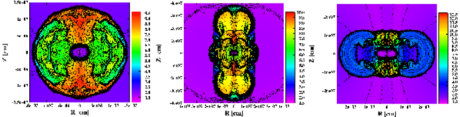
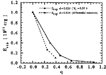
5.4.2 anisotropic neutrino radiation in rotational core-collapse

Then the problem is whether rotation does good or harm to the neutrino-driven mechanism. K. Sato’s group in University of Tokyo has been paying attention to the effect of rotation on the neutrino heating mechanism. First of all, Shimizu et al. (2001) [272] demonstrated that anisotropic neutrino radiations induced by rotation may be able to enhance local heating rates near the rotational axis and trigger globally asymmetric explosions. The required anisotropy of the neutrino luminosity appears to be not very large ($\sim 3\%$). In their study, the anisotropy of neutrino heating was given by hand and rotation was not taken into account, either. Kotake et al. (2003) [175] demonstrated how large the anisotropy of neutrino radiation could be, based on the two dimensional rotational core collapse simulations from the onset of gravitational collapse of the core through the core bounce to the shock-stall . In their study, a tabulated EOS based on the relativistic mean field theory [287] was implemented and the electron captures and neutrino transport was approximated by the so-called leakage scheme. They not only estimated the anisotropy of neutrino luminosity but also calculated local heating rates based on that. In the following, we state the main results shortly.

In the left panel of Figure 90, the neutrino spheres after the shock-stall ($\sim 50$ msec after core bounce) for the spherical and the rotating model (corresponding to model A in Figure 87) are presented. For the rotating model, it is found that the neutrino sphere forms deeper inside at the pole than for the spherical model. This is a result of the fact that the density is lower on the rotational axis in the rotation models than in the spherical model because the matter tends to move away from the axis due to the centrifugal force. The neutrino temperature profile on the neutrino sphere for the pair models is presented in the right panel of Figure 90. Note that the neutrino temperature is assumed to be equal to the matter temperature. It is seen from the figure that the temperature varies with the polar angle for the rotating model. The neutrino temperature is higher at the pole for the rotating model than for the spherical model. This can be understood from the fact that the neutrino sphere is formed deeper inside for the rotational model than for the spherical model, as mentioned above.

Figure 90: Shapes of neutrino sphere (left panel), neutrino temperature vs. polar angle on the neutrino sphere (right panel) for the rotating and the spherical models. These figures are taken from [175]

Based on the above results, the heating rates of the charged-current interaction: $\nu_{e}+n\rightarrow p+e^{-}$ outside the neutrino sphere were estimated. The neutrino emission from each point on the neutrino sphere is assumed to be isotropic and take a Fermi-Dirac distribution with a vanishing chemical potential. For the details about the estimation, we refer readers to [175]. In Figures 91 and 92, the contour plots of the heating rate for the above two models and the neutrino heating rate along the rotational axis with that on the equatorial plane for the rotating model are presented, respectively. It is clearly seen from the figure that the neutrino heating occurs anisotropically and is stronger near the rotational axis for the rotation models. This is mainly because the neutrino temperatures at the rotational axis are higher than on the equatorial plane. In addition, the radius of the neutrino sphere tends to be smaller in the vicinity of the rotational axis. As a result, the solid angle of the neutrino sphere is larger seen from the rotational axis. These two effects make the neutrino heating near the rotational axis more efficient.

Figure 91: Heating rates outside the neutrino sphere for the spherical model (right) and the rotating model (left). The color scale is the logarithm of the heating rate ($\rm{MeV}~{}\rm{nucleon}^{-1}~{}\rm{s}^{-1}$). The neutrino sphere and the stalled shock are seen as the thick lines separating the bright color from the dark color region. Note that the value within the neutrino sphere is artificially modified to dark colors and has no physical meanings. These figures are taken from [175].

Figure 92: The comparison of the heating rate ${Q^{+}}_{\nu}\,\,(\rm{MeV}/(\rm{nucleon}\cdot\rm{s}))$ along the rotational axis with that on the equator for the rotating model. The pole-to-equator ratio of the heating rate outside the neutrino sphere is about 3. These figures are taken from [175].

Figure 93: Possible consequence of anisotropic neutrino radiation from the central protoneutron star, with the surface temperature of 4.5 MeV with 10 $~{}\%$ neutrino flux enhancement along the rotational axis treated as the lightbulb approximation. The color map shows the dimensionless entropy distribution and the velocity fields (left $t=82~{}{\rm msec}$ and right $t=244~{}{\rm msec}$ after the shock stall). This figure is taken from Madokoro et al. (2003) [221].

Figure 94: Critical luminosity for the accretion shock revival as a function of the accretion rate. Solid line denotes the spherical model, and the other lines correspond to the rotating models with the different initial angular velocities ($\Omega=0.03~{}\rm{rad}~{}\rm{s}^{-1}$; dotted line and $0.1~{}{\rm rad}{\rm s}^{-1}$; dashed line). It can be seen that the rotation can lower the critical luminosities for a give accretion rate. These figures are taken from [370].

Figure 95: Density isosurface ($10^{11}~{}{\rm g}~{}{\rm cm}^{-3}$ (blue), $10^{12}~{}{\rm g}~{}{\rm cm}^{-3}$ (red)) implying the shapes of the neutrino spheres obtained in the 3D rotational core-collapse simulations by Fryer and Warren (2004) [101] (at 45 msec after core bounce in model SN15BB-hr). It is shown that their shapes are deformed to be oblate and the aspect ratios of the neutrino spheres are about $\sim$ 2.

Figure 96: Left is the snapshots of the stellar structure for a rotating model ($\Omega=0.5~{}{\rm rad}~{}{\rm s}^{-1}$ imposed on $15M_{\odot}$ progenitor model) at 198 msec after core bounce. The left panels show the rotational velocity (top) and the fluctuations of entropy (in percent) versus the enclosed mass, emphasizing the conditions inside the neutron star. The right panels display the rotational velocity (top) and the entropy as functions of radius. The arrow indicate the velocity field and the white line marks the shock front. Right panel shows the shock radii ($R_{s}$) vs. postbounce time ($t_{\rm pb}$). The 2D models are compared to the corresponding 1D simulations (thin lines). These figures are taken from Buras et al (2003) [45].

Figure 97: Integrated net gain (in unit of ${\rm erg}~{}{\rm g}^{-1}~{}{\rm s}^{-1}$) in the rotational core-collapse simulations with multigroup neutrino transport with a flux limitter. $\Omega_{0}$ in each panel shows the initial angular velocity of the core. The inner region 600 km on a side is shown. With increasing initial angular velocity, the heating rate is shown to be more and more concentrated along the rotational axis. This figure is taken from Walder et al (2005) [342].

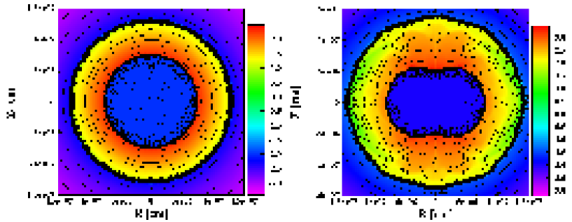
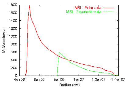
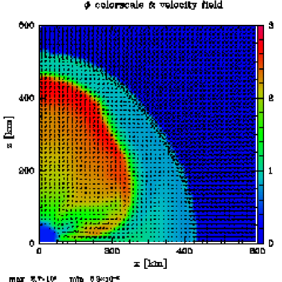
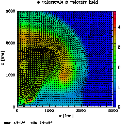
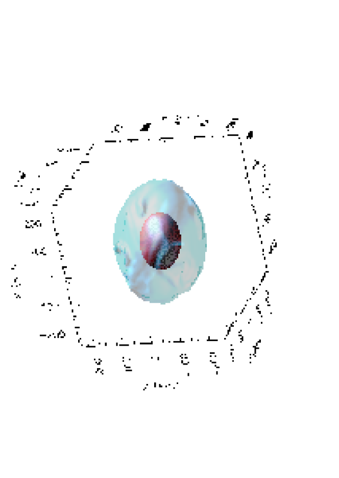
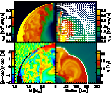
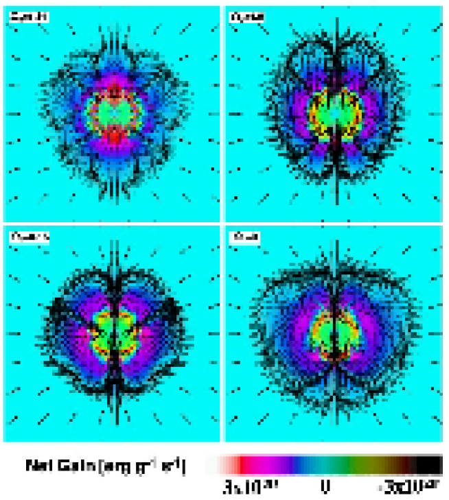
By performing the linear analysis for the convective stability in the corresponding models, it was found that the convective regions appear near the rotational axis (see [175] and [100]). This is because the gradient of the angular momentum is rather small near the axis and the stabilizing effect of rotation is reduced there. The neutrino heating enhanced near the rotational axis might lead to even stronger convection there later on. Then, the outcome will be a jet-like explosion as considered in [272, 221, 222] (see Figure 93). Here it should be mentioned that such jet like explosions play important roles in reproducing the synthesized abundance patterns of SN1987A [248, 249].

Yamasaki and Yamada (2005) [370] recently reported the steady accretion flows onto the protoneutron star with a standing shock, in which they investigated how rotation affects the critical luminosity required for the shock revival. Note that this study is the extension of the study by [49], in the sense that the former newly takes into account the effect of rotation. For a given mass accretion rate, they found that rotation does lower the critical luminosity than the one in the case of the spherically symmetric mass accretion (see Figure 94). This result is also in favor of rotation for producing the successful explosions.

A series of SPH simulations in 2D or 3D of rotational core-collapse has been done by [100, 101]. They referred to the deformation of the neutrino sphere induced by rotation (see figure 95). However, little effect of neutrino anisotropy on the explosion was found. This is probably their models explode in the prompt-shock timescale.

Buras et al. (2003) [45] reported the core-collapse simulations of a slowly rotating model, in which the state-of-the-art neutrino reactions are included with the multigroup neutrino transport along the radial rays. Although the shock wave reaches further out in the rotating model than the one in the spherically symmetric model, the shock wave in the rotating model is shown to stall in the iron core (compare “s15r” (rotating model) and “s15” (spherical model) in the right-down panel of Figure 96).

Very recently, Walder et al (2005) [342] reported the two-dimensional rotating core-collapse simulations, in which the multi-energy neutrino transport with the flux-limited diffusion approximation was employed, and calculated the anisotropies of the neutrino flux in the rotating cores (see Figure 97). The degree of the anisotropy obtained in their simulations is almost the same with the aforementioned results [175] when the initial rotational velocity of the core are close with each other. In addition, they pointed out that the degree of the anisotropy becomes much smaller if the core rotates rather slowly as suggested by the recent stellar evolution calculation [122] and thus concluded that the rotation-induced neutrino heating anisotropy could not be a pivotal factor in the supernova explosion mechanism.

Here it should be mentioned that the lateral neutrino heating, which is essential for the anisotropic neutrino radiation to work, can neither treated very appropriately by the neutrino transport along the radial rays [45] nor by the flux-limited diffusion approximation [342]. Especially the diffusion approximation could lead to the underestimation of the anisotropy ratios. The fully spatially multidimensional radiation-hydrodynamic simulations seem required to give us the answer whether the anisotropic neutrino radiation does really help the explosion.

Figure 98: Convection inside the rotating protoneutron stars. In the left panel, the contour of the absolute value of the fluid velocity evolved about 750 msec after core bounce evolved by a numerical simulation [151] is shown. From the panel, the convection is shown to be suppressed near the rotational axis (vertical) and develop strongly near the equatorial plane. In the right panel, the direction, to which the convective motions are likely to occur at 500 msec after core bounce, is shown, which is obtained by a stability analysis [245]. The convection is more effective in the polar region. The left and right panel is taken from Janka & Keil (1997) [151] and Miralles et al (2004) [245], respectively.

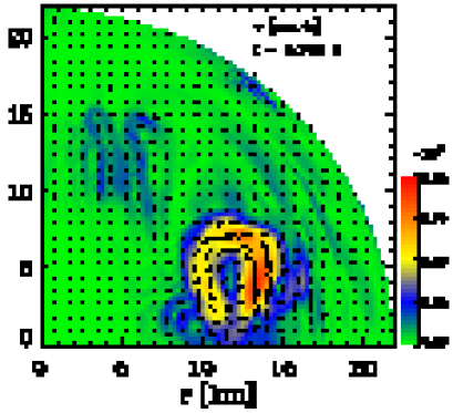
5.4.3 convection in rotating protoneutron stars

As in the non-rotating cases, rotation should affect the convective unstable regions in the protoneutron stars (PNSs). Janka and Keil (1997) [151] performed the two-dimensional hydrodynamic simulation in the PNS treating the neutrino transport in the grey flux-limited diffusion approximation and pointed out that convections occurs only close to the equator (see the left panel of Figure 98). On the other hand, a recent study by Miralles et al. (2004) [245] suggests that the convective unstable regions are formed along the direction of the rotational axis preferentially (the right panel of Figure 98). Note that the computations by [245] are based on the linear stability and only valid in a steady-state situation, which is not always satisfied in the PNS. The results between the two studies, namely, the appearance of the convective regions seems to change with the time evolution of the PNSs [245]. The effects of the heating anisotropy produced by the convections inside the rotating PNSs on the explosion mechanism are still an open question.

As mentioned, the recent evolution models by [122] suggest that the transport of angular momentum during the quasi-static evolutionary phase of the progenitor deprives the core of substantial fraction of its angular momentum, particularly when the magnetic torque is taken into account [273]. If this is really the case, the rotation will play no significant role in dynamics of core-collapse as shown by [45, 242, 342].

5.5 Roles of Magnetic Fields

Another possible cause for the asphericity of supernovae may be magnetic fields. Soon after the discovery of pulsars, which are the magnetized rotating neutron stars, the role of rotation plus magnetic fields in the supernova explosion was scrutinized [257, 37]. Because of the magnetic flux conservations, a seed magnetic field in the stellar core can grow significantly during core-collapse. In addition, winding of field lines due to the differential rotation, which is natural after the collapse of a spinning core, can further amplify the toroidal field component. If the magnetic pressure becomes comparable to the thermal pressure, magnetohydrodynamical forces can drive an explosion [238], and accelerate axial jets [246, 274, 195, 12]. Also magnetic buoyant instabilities could produce mass motions along the rotational axis. It should be mentioned that the necessary condition for the working of the above mechanisms is that the core should be very strongly magnetized initially. The magnetic field strength is required to be more than $\sim 10^{16}$G if the magnetic stress is to be comparable to the matter pressure in the supernova core after core bounce. Since the canonical value for the pulsar, $\sim 10^{12}$G, is negligibly small in terms of the above effects on the dynamics of collapse, little attentions have been paid to the magnetic supernovae.

However, it has been recently recognized these days that some neutron stars are indeed strongly magnetized as high as $B\geq 10^{14}$ G. The strong dipolar magnetic fields at the surface can be estimated as follows,

$$B_{\rm dipole}\sim 3.0\times 10^{14}\sqrt{\frac{P\dot{P}}{10^{-10}~{}{\rm s}}}~{}[{\rm G}],$$ (251)

which is distinct from the normal radio pulsars by their long periods ($P$) and high-period derivatives ($\dot{P}$). Some of them are soft gamma repeaters (SGRs) and others are anomalous X-ray pulsars (AXPs) or high magnetic field radio pulsars (HBPs) [371, 115], which are collectively referred to as “magnetars” [84] (see Figure 99 and [361] for review of the current observations). Although they are supposed to be a minor subgroup of neutron stars and the field strength might be lowered to the normal pulsars [146], these situations do revive the study of the magnetic supernova again [368, 178, 326, 268, 179].

Figure 99: $B_{p}-P$ diagram of radio pulsars and known magnetars taken from [371]. The number of the magnetars discovered so far is about 10. See for details [371].

5.5.1 effect of magnetic fields on the prompt shock propagation

As in the case of rotation [366], the first step to be investigated is the effect of magnetic fields (in combination with rotation) on the dynamics of the prompt propagation of a shock wave [368, 326].

The recent 2D magnetohydrodynamic simulations by Yamada & Sawai [368] and Takiwaki et al [326] showed that the combination of rapid rotation, $T/|W|\geq 0.1\%$ and strong poloidal magnetic field, $E_{\rm m}/|W|\geq 0.1\%$, leads in general to jet-like explosions. Here $T/|W|$ and $E_{\rm m}/|W|$ represents the initial ratio of the rotational and magnetic energies to the gravitational energy, respectively. $E_{\rm m}/|W|\geq 0.1\%$ roughly means that the iron core has $B\geq 10^{12}~{}{\rm G}$ before the onset of gravitational core-collapse. In the following, we describe the magnetohydrodynamics features in such strongly magnetized and rapidly rotating models.

The typical time evolutions are presented in Figure 100. The initial $T/|W|$ and $E_{\rm m}/|W|$ imposed initially on the model is 1.5 $\%$ and 1.0 $\%$, respectively. The initial field configuration is assumed to be parallel to the rotational axis with $B_{0}=5.8\times 10^{12}~{}{\rm G}$. After core bounce, the fast magnetohydrodynamic shock is launched in the direction of the rotational axis. From Figure 101, it can be seen that a seed magnetic field grow significantly during core-collapse due to the magnetic flux conservation (see the right panel of Figure 101 from A to C). Before core bounce (point C), the poloidal magnetic fields dominate over the toroidal ones. After core bounce, winding of field lines due to the differential rotation near the surface of the inner core can drastically amplify the toroidal components (see the right panel of Figure 101 after point C). In Figure 102, the properties of the shock wave propagating further out from the central region are presented. From the top left panel, the shock wave produced after core bounce becomes magneto-driven, in the sense that the magnetic pressure becomes as strong as the matter pressure behind the shock wave (see the top right panel of Figure 102). Note that the magnetic pressure is much smaller than the matter pressure in the unshocked inner core due to its high density, however, can be much larger in the distant region from the center, because the matter density drops much steeper than the magnetic fields which is almost constant along the rotational axis. The magneto-driven shock wave is shown to be collimated along the rotational axis because the the hoop stress $F_{\rm hoop}=\frac{B_{\phi}^{2}}{X}$, which collimates the shock wave, is dominant over the gradient of the magnetic pressure, $F_{\rm mag}=\frac{1}{2}\frac{\partial B_{\phi}^{2}}{\partial X}$, acting to expand the shock wave (see the bottom panel of Figure 102). Here $X$ represents the distance from the rotational axis. These are the reasons for producing the jet-like explosion.

Figure 100: Velocity fields (upper panels) and the poloidal magnetic fields (lower panels, white lines) on top of the density contours ($\log_{10}\rho$). Left and right is for core bounce and for 10 msec after core bounce. These figures are taken from Yamada and Sawai (2004) [368].

Figure 101: Left panel is the time evolution of the central density and right is the time evolution of mean poloidal (dotted) and toroidal (solid) magnetic fields for a typical MHD model. Comparing the panels, one can see that “C” represents the time of core bounce. After core bounce, the toroidal component dominates over the poloidal one. These figures are taken from Sawai et al. (2005) [268].

Figure 102: A jet like explosion obtained in the rapidly rotating and strongly magnetized model studied in Takiwaki et al (2005) [326]. Top left panel shows the contour of the entropy per nucleon near the shockbreak out of the iron core showing a jet like explosion. Top right panel shows the contour of the logarithm of the plasma beta, $\beta$, which is the ratio of the magnetic to matter pressure, representing that the shock wave is magneto-driven, since $\beta$ is greater than 1 just behind the shock wave. Bottom panel shows the contour of the ratio of the hoop stress to the gradient of the magnetic pressure, which demonstrates that the shock wave is collimated by the hoop stress near the rotational axis.

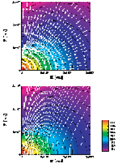
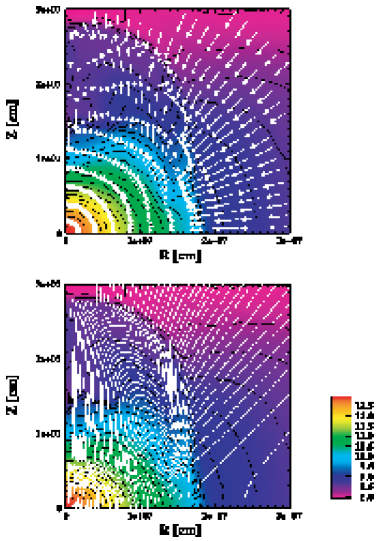
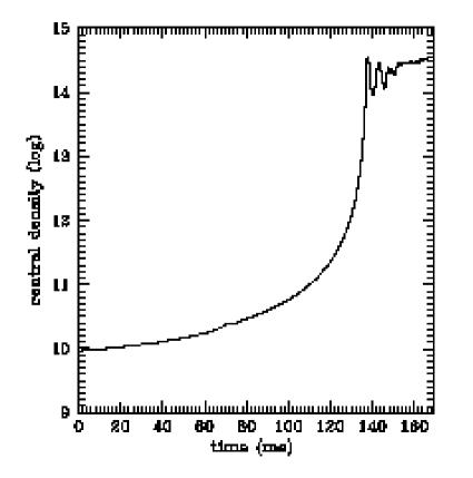
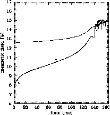
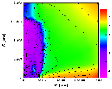
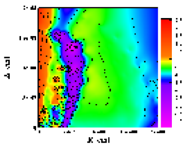
Furthermore it was pointed out that the explosion energy increases with the initial magnetic fields strength, on the other hand, monotonically decreases with the the initial rotation rate [326]. This is because the collimated shock wave requires relatively lower energy to expel the matter near the rotational axis as the initial field strength becomes larger. As a result, the stronger initial magnetic field is favorable to the robust explosion. Interestingly, the models with the smallest magnetic fields studied in [368, 326] still produced the jet-like explosion although it takes longer for winding up the fields to launch the jet. This might suggest that even much smaller magnetic fields could be amplified in the collapsed core and play an important role for explosion.

5.5.2 possible mechanisms for producing the pulsar-kicks

During core-collapse of such strongly magnetized models, the strength of the magnetic fields substantially exceeds the QED critical value, $B_{\rm QED}=4.4\times 10^{13}$ (G), above which the neutrino reactions are affected by the parity-violating corrections to the weak interaction rates [143, 15, 16, 10]. Kotake et al. (2005) [178] estimated the corrections based on the results in the 2D MHD simulations and discussed its role for producing the pulsar kicks, which will be summarized shortly below (see also [185, 186, 184] for a review).

Figure 103: Various quantities for a model with the strong magnetic fields and rapid rotation initially (see the context for the details of the model). Top left panel shows contour of the logarithm of the poloidal magnetic fields ($\log[B_{p}~{}{(\rm G})]$) with the magnetic field lines. Top right panel represents the ratio of the neutrino heating rate corrected from the parity-violating effects, $\Delta Q_{\nu,\rm{B}\neq 0}^{+}$ to the heating rate without the corrections, $Q_{\nu,\rm{B}=0}^{+}$. Note in the panel that the values of the color scale are expressed in percentage and that the central black region represents the region inside the neutrino sphere. Bottom right panel is the same with the top right panel except that the bottom right panel only shows the regions with the negative values of the ratio. Thus the white region shows the regions with the positive values of the ratio. Bottom left panel shows the contour of the ratio in the whole region, which is prepared in order to see the global asymmetry of the heating induced by the strong magnetic fields. These figures are taken from Kotake et al (2005) [178].

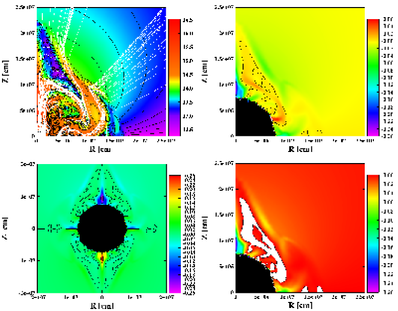
In the top left panel of Figure 103, the configuration of the poloidal magnetic fields after the shock stall ($\sim 50$ msec after core bounce) is presented. For the initial condition for the model, the strong poloidal magnetic fields of $2\times 10^{12}$ G was imposed with the high angular velocity of 9 $\rm{rad}/\rm{s}$ with a quadratic cutoff at 100 km radius in the iron core. It is seen from the panel that the poloidal magnetic fields are rather straight and parallel to the rotational axis in the regions near the rotational axis, on the other hand, bent in a complex manner, in the other central regions due to the convective motions after core bounce. The top right panel of Figure 103 shows the ratio of the neutrino heating rate corrected from the parity-violating effects, $\Delta Q_{\nu,\rm{B}\neq 0}^{+}$ to the heating rate without the corrections, $Q_{\nu,\rm{B}=0}^{+}$. It is noted that the suppression or the enhancement of the heating rate through parity-violating effects is determined by the signs of the inner product of ${\mbox{\boldmath$\hat{n}$}}\cdot\mbox{\boldmath$\hat{\rm{B}}$}$, where $\hat{n}$, $\hat{\rm{B}}$ are the unit vector in the direction of the incoming neutrinos and along the magnetic field. If the product is positive (negative), then the corrections to the heating rates results in the suppression (enhancement) of the heating rate. Reflecting the configurations of the magnetic fields, it is seen that the values of the ratio become negative in almost all the regions (see also the bottom right panel of Figure 103 for clarity). This means that the heating rate is reduced by the magnetic fields than that without. Especially, this tendency is most remarkable in the regions near the rotational axis and the surface of the neutrino sphere (see the regions colored by blue in the top right panel of Figure 103). This is because the magnetic fields are almost aligned and parallel to the rotational axis in the regions near the rotational axis. In the bottom left panel of Figure 103, the contour of the ratio in the 360 latitudinal degrees region of a star, is prepared in order to see the global asymmetry of the heating. Since their simulations assumed the equatorial symmetry, the above features in the northern part of the star become reverse for the southern part. As a result, it was found that the heating rate is reduced about $\sim 0.5\%$ in the vicinity of the north pole, on the other hand, enhanced about $\sim 0.5\%$ in the vicinity of the south pole in the computed model in [178]. If the north/south asymmetry of the neutrino heating persists throughout the later phases, it is expected that the pulsar is likely to be kicked toward the north pole.

There is an another class of the mechanism for producing the kicks, which relies on the cause of the asymmetric explosion as a result of the global convective instabilities [51, 112, 102] caused by the pre-collapse density inhomogeneities [31] (see Figures 105, 105) or the local convective instabilities [155] formed after the onset of core-collapse. More recently, Scheck et al [269]. recently pointed out that the random velocity perturbation of $\sim 0.1$ % added artificially at several milliseconds after bounce could lead to the global asymmetry of supernova explosion and cause the pulsar-kick (see Figure 106). While the orientation of pulsar-kicks is stochastic in their models, which is truly consistent with the observation of the normal pulsars, the asymmetry of the neutrino heating in the strong magnetic fields mentioned above might predict the alignment of the magnetic axis and the kick velocity in highly magnetized neutron stars.

Figure 104: Density inhomogenties (left) produced during oxygen shell burning and their root-mean-square azimuthal averages (right). These figures are taken from Bazan and Arnett (1998) [31].

Figure 105: Kick velocities ($x,y,z$ directions) of the neutron star due to the density inhomogenities prior to collapse. The inhomogenities were parametrically imposed in two ways, namely on the oxygen shell only and the core oscillation, with the density variations of $\leq 25\%$. After the oscillatory behaviors, which were pointed out to be due to the neutrino emission from material accreting onto the neutron star, the motions of the neutron star tend to damp in time with the kick velocity less than $200~{}{\rm km}~{}{\rm s}^{-1}$. This figure is taken from Fryer (2004) [102].

Figure 106: The global asymmetry of $l=1$ mode and the kick velocities of the protoneutron star. Left panel shows the growth of $l=1$ at 1 s after core bounce. In the right panel, the velocities of the neutron star (top) and the explosion energies (bottom) as a function of time measured from core bounce are given for some representative models (see [269] for details). At 1 s, it can be seen that the kick velocity becomes as high as $\sim 600$ km/s in one of the models wit the explosion energy of $\sim 1\times 10^{51}$ erg. These figures are taken from Scheck et al (2004) [269].

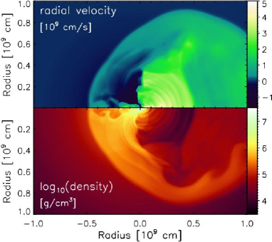
5.5.3 effect of toroidal magnetic fields

While most of the magnetohydrodynamic (MHD) simulations in the context of core-collapse supernovae choose poloidal magnetic fields as initial conditions [195, 37, 246, 238, 274, 12, 368], recent stellar evolution calculations show that toroidal magnetic fields may be much stronger than poloidal ones prior to collapse [121, 122, 273]. Motivated by this situation, Kotake et al (2004) investigated the models with predominantly toroidal magnetic fields, changing the strength of rotation and the toroidal fields systematically.

The angular velocity profile for the model with the strongest toroidal magnetic fields in their simulations is given in the top left panel of Figure 107. The initial values of $T/|W|$ and $E_{\rm m}/|W|$ are $0.5,0.1\%$, respectively, where $E_{\rm m}/|W|$ represents magnetic to gravitational energy. In addition, the initial profiles of rotation and magnetic field are chosen to be cylindrical with strong differential rotation for this model.

Figure 107: Contour plots of various quantities for the model with the strongest magnetic field in the computations [177]. The top left panel shows the logarithm of the angular velocity ($\rm{s}^{-1}$). The top right panel represents the magnetorotationally unstable regions to non-axisymmetric perturbations. The plot shows the growth time scale (s) of MRI. Note in this panel that the regions with white represent stable regions against MRI. The bottom left panel shows the logarithm of magnetic field strength (G). The bottom right panel displays the logarithm of the ratio of magnetic stress to matter pressure in percentage.

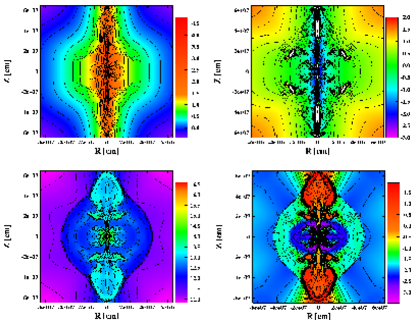
In the top left panel, the negative gradient of angular velocity, $d\Omega/dX<0$, can be found, where $\Omega$ is the angular velocity and $X$ is the distance from the rotational axis. Such a region is known to be unstable to non-axisymmetric perturbations [26, 4], as will be discussed in subsections of 5.5.4 and 5.5.5. The characteristic time scale for the growth of the instability called the magnetorotational instability (MRI) is given as $\tau_{\rm MRI}=4\pi|d\Omega/d\log X|^{-1}$. The top right panel of Figure 107 shows the contour of $\tau_{\rm MRI}$ for the model. The typical time scale is found to be $\sim O(10)$ ms near the rotational axis. This suggests that MRI induced by non-axisymmetric perturbations can grow on the prompt shock time scale. The field strengths in the protoneutron star become as high as $\sim 10^{16}$ G (see the bottom left panel of Figure 107), and the ratio of magnetic stress to matter pressure gets as high as $0.9$ behind the shock wave (see the bottom right panel of Figure 107).

As for the anisotropic neutrino radiation observed in purely rotating case (subsection 5.4.2), the feature is shown to be not changed significantly by the inclusion of very strong toroidal magnetic fields ($\sim 10^{16}$ G in the protoneutron star). Combined with the anisotropic neutrino radiation that heats matter near the rotational axis more efficiently the growth of the instability is expected to further enhance heating near the axis. Furthermore, the magnetic pressure behind the collimated shock wave is as strong as the matter pressure in the vicinity of the rotational axis. From these results, one might speculate that the magnetar formation is accompanied by a jet-like explosion if it is formed in the magnetorotational collapse described above.

5.5.4 foundations of magnetorotational instability

Figure 108: Schematic figure prepared for the derivation of the growth condition of MRI. When the radial displacement of $\Delta r$ of the fluid element is imposed, the MRI develops if the sum of the gravity and the centrifugal force becomes larger than the magnetic tension (see text for details).

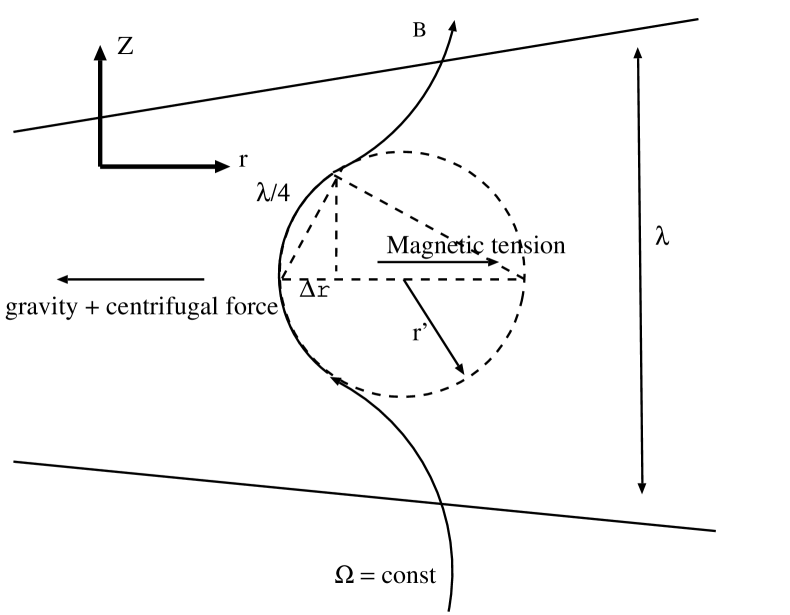
So far in this section, we have concentrated on the models which have large magnetic fields prior to core-collapse. The most mysterious is the origin of this large magnetic field. The core might have strong magnetic fields prior to collapse already, although the evolution models indicate quite the contrary [122]. We may not need the strong magnetic field initially if the magnetorotational instability (MRI) sufficiently develops in the supernova core. This MRI was first discussed in the context of accretion disks by [26]. Before we mention the role of MRI in the supernova, we summarize, for convenience, the basic properties of MRI in the context of accretion disks around the black hole, which are common situations in the central part of the active galactic nuclei.

First of all, let us derive the growth condition for the MRI. See a schematic Figure 108, describing the small displacement of the magnetic fields in the accretion disk. Before the displacement, the magnetic fields with strength $B$ are assumed to be uniform and parallel to the rotational axis of the disk ($z$ axis). The displacement is assumed to occur at the radial distance $r$ from the central region of density $\rho$. Furthermore, let us assume that the disk is in a Kepler rotation, namely, the angular velocity of the disk yields,

$$\Omega=\sqrt{\frac{GM}{r^{3}}},$$ (252)

where $M$ is the mass of the central object, presumably the black hole.

As in the Figure 108, let us displace the fluid element $\Delta r$ inwards. Since the ideal MHD approximation can be well satisfied in the accretion disks, the magnetic fields are frozen-in to the matter. Thus the field line also moves $\Delta r$ inwards as in Figure 108. Since the angular velocity of the magnetic field is constant, the centrifugal force becomes smaller due to the displacement. The change of the centrifugal force can be written,

$$\delta F_{\rm rot}=(r-\Delta r)\rho\Omega^{2}.$$ (253)

On the other hand, the gravity in the radial direction increases,

$$\delta F_{\rm grav}=-\frac{\rho GM}{r^{2}}\Bigl{(}1+2\frac{\Delta r}{r}).$$ (254)

As a result, the net force in combination of the centrifugal force and the gravity becomes,

$$\delta F_{\rm tot}=\delta F_{\rm rot}+\delta F_{\rm grav}=-3\rho\Omega^{2}\Delta r,$$ (255)

which acts to move the displaced field line inwards. If this force is stronger than the magnetic tension, which acts to put the displacement back, the instability develops. The magnetic tension is $B^{2}/r^{{}^{\prime}}$, here $r^{{}^{\prime}}$ is the curvature radius of the magnetic field (see Figure 108). From a simple geometric calculation, one can obtain the magnetic tension,

$$\delta F_{\rm mag}=\frac{B^{2}}{r^{{}^{\prime}}}=\frac{2B^{2}\Delta r}{(\lambda/4)^{2}},$$ (256)

where $\lambda$ is the wavelength of the perturbation. Thus the condition for the growth of the instability becomes,

$$\delta F_{\rm mag}+\delta F_{\rm top}=\Bigl{(}\frac{2B^{2}}{(\lambda/4)^{2}}-3\rho\Omega^{2}\Bigr{)}\Delta r<0.$$ (257)

As a result, the wavelength of the perturbation satisfying the condition $\lambda>\lambda_{c}=4\sqrt{2/3}v_{\rm A}/\Omega$ becomes unstable, where $v_{A}$ is the Alfvén velocity defined as $v_{\rm A}=\frac{B}{\sqrt{4\pi\rho}}$. This is the condition for the onset of the MagnetoRotational Instability (MRI).

Growth rate of the MRI can be roughly estimated as

$$\eta_{\rm growth}\sim\frac{v_{\rm A}}{\lambda_{c}}.$$ (258)

To investigate the dependence of the growth rate on the wavelength of the perturbation, one need more detailed analysis (see for a review [26]) than the one done above. In Figure 109, the dispersion relation between the frequency ($\omega$) and the wavenumber ($k_{z}$ : along the unperturbed magnetic field) of perturbations is shown. The above relation was found by the linear analysis by adding the axisymmetric perturbations to the Keplerian disk with uniform magnetic fields parallel to the rotational axis and with the assumption that the fluid is incompressible (see for detail [27]). The oscillation, which is marginally stable ($\omega=0$) in the absent of the magnetic fields, is shown to be unstable ($\omega<0$) in the presence of the magnetic fields. The maximum growth rate (minimum of the curve in Figure 109) is shown to be,

$$\eta_{\rm max}=\frac{3}{4}\Omega,$$ (259)

with

$$k_{z}v_{\rm A}=\sqrt{\frac{15}{16}}\Omega.$$ (260)

Since this is very rapid indeed, the amplitude with the unstable mode can be significantly amplified during several rotation periods. The MRI can amplify the fields even if the initial field is very weak. It should be noted that the growth rate is independent of the strength of the magnetic field. Instead, the growth rate of MRI is determined by the angular velocity (see Eq. (259)). This is the main characteristic of the MRI, which is distinct from other magnetic instabilities such as Parker instability. As the MRI develops, the initial poloidal magnetic fields are stretched to the toroidal ones, whose strength grows exponentially with time. It is noted that the MRI can also develop nonaxisymmetrically. The evolution of the magnetic energy due to the nonaxisymmetric MRI in the accretion disk threaded by the purely toroidal fields is shown in Figure 110. The MRI and its associated angular momentum transport have been paid great attention in the community of the accretion disks around the black hole.

Figure 109: The growth rate of MRI again axisymmetric perturbations in the incompressible and magnetized disk with a Kepler rotation. In the region with $\omega<0$, the MRI develops. This figure is taken from Balbus & Hawley (1991) [27].

Figure 110: The spatially averaged magnetic energy normalized by the gas pressure as a function of the rotation period of the accretion disk obtained in the 3D simulations of accretion disk threaded by the toroidal magnetic fields. $\beta_{0}$ represents the initial value of the plasma beta imposed on the disk. It can be seen that the magnetic energy increases exponentially regardless of the initial $\beta_{0}$ and reaches to the quasi-steady state with $P_{\rm gas}/P_{\rm mag}\sim 10$. This figure is taken from Matsumoto et al (1999) [224].

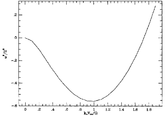
5.5.5 possibility of the growth of magnetorotational instability in supernovae

Figure 111: The angular velocity (left panel) and the saturation magnetic fields (right panel) as a function of radius taken from Akiyama et al (2003) [4]. It is seen from the left panel that at core bounce, the angular velocity decreases sharply with the radius near $r\sim 10$ km, where is near the surface of the protoneutron star. This negative gradient of the angular velocity ($d\Omega/dr\leq 0$) is the criteria for the onset of the MRI (see [26] for its derivation). They pointed out that the magnetic fields could be amplified as high as $10^{16}$ G in the later phases as shown from the right panel.

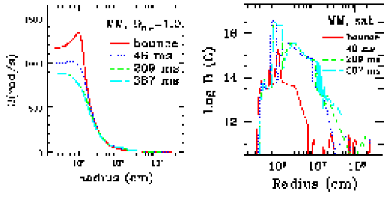
The MRI mentioned in the last subsection was first applied to the dynamics of supernova core by Akiyama et al (2003) [4]. Compared with the linear growth of the toroidal magnetic fields in case of field wrapping, the field is expected to grow exponentially due to MRI also in the supernova core. If it is true, we may need the only small seed magnetic fields. When MRI develops efficiently in the supernova core, the field might reach to the saturation strength, which is estimated to be as high as

$$B_{\rm sat} = (4\pi\rho)^{1/2}r\Omega$$ (261)

$$\sim 4\times 10^{16}\Bigl{(}\frac{\rho}{1\times 10^{13}~{}{\rm g}~{}{\rm cm}^{-3}}\Bigr{)}^{1/2}\Bigl{(}\frac{R}{10~{}{\rm km}}\Bigr{)}\Bigl{(}\frac{\Omega}{1000~{}{\rm rad}~{}{\rm s}^{-1}}\Bigr{)}~{}[{\rm G}],$$

where we employ the typical values near the surface of the protoneutron star (see Figure 111). Here the saturation field is determined by the condition that the toroidal component of the Alfvén speed, $v_{\rm A}=\frac{B}{\sqrt{4\pi\rho}}$, comes into rough equipartition with the rotation velocity, $v_{\rm rot}=r\Omega$, in analogy with the case in the accretion disk [26].

In such a case, the magnetic stresses generated by the MRI could be the origin of the viscous energy deposition [332]. By employing an $\alpha$ prescription for the viscous dissipation, which is often used in the study of accretion disk [270], the robust explosion was pointed out to be obtained because the MRI heating aids the neutrino heating (see Figure 112).

Figure 112: Effect of viscous heating due to MRI on the explosion mechanism taken from Thompson et al. (2005) [332]. Left panel shows the energy deposition rate as a function of radius for a rotating model with the initial period of $2$ seconds, including viscous heating via the MRI with $\alpha=0.1$. In this panel, total energy deposition rate ($\dot{q}_{\rm tot}=\dot{q}_{\nu}+\dot{q}_{\rm MRI}$, solid line), viscous energy deposition ($\dot{q}_{\rm MRI}$, dot-dashed line), and neutrino deposition rate from each species ($\nu_{e}$ short-dashed line, $\bar{\nu}_{e}$ dotted line) are shown. The order of 10 % increase of the heating rate due to the viscous heating above the gain radius ($R\sim 120~{}{\rm km}$) can be seen. This increase was pointed out to be sufficient to instigate the explosion. Right panel shows the various timescales of the same model in the left panel. $\tau_{H_{\nu}}$, $\tau_{C_{\nu}}$, $\tau_{\dot{q_{\nu}}}$, $\tau_{\rm adv}$, $\tau_{\rm MRI}$, and $\tau_{\dot{q_{\rm TOT}}}$, represent the timescales of neutrino heating, neutrino cooling, the advection of the infalling matter, the viscous heating of MRI, the total heating including the contributions of MRI, as a function of radius, respectively. $R_{\nu_{e}}$ and $R_{\rm g}$ mark the position of the $\nu_{e}$ neutrinosphere and the gain radius, respectively. In the regions above the gain radius from $130{\rm km}<R<\sim 170~{}{\rm km}$, the net heating time scale becomes shorter than the advection timescale of the infalling matter as a result of the viscous heating. Otherwise in the slowly rotating models $P_{0}>5~{}\rm{s}$, the explosions were not obtained in their computations, because there are no regions, in which the condition, $\tau_{\dot{q}_{\nu}}<\tau_{\rm adv}$, is satisfied.

Although there remains persistent concern of the treatment of the rotation and magnetic fields in the above 1D model computations [4, 332], the obtained implications seem to be important and should be examined by the multidimensional MHD simulations [332]. Currently the 3D MHD simulations have just begun to be investigated (see, for example [200]). Very recently nucleosynthesis in the magnetic supernovae has been reported [251]. Although the study of magnetic supernovae is still in its infancy with respect to the treatment of the neutrino physics, this field seems to be blossoming with the recent developments both of the transport method [45, 202, 342] and the growing computing power.

6 Gravitational Waves from Core-Collapse Supernovae

From this section, we review the studies about gravitational waves from core-collapse supernovae. As mentioned in section 1, the detection of the gravitational signal is important not only for the direct confirmation of general relativity but also for the understanding of the explosion mechanism supernovae themselves. In combination with neutrino signals mentioned in section 4, the gravitational wave will enable us to see directly the innermost part of an evolved star, where the key physics related to the explosion mechanism such as the angular momentum distribution and the equation of state are veiled.

In this section, we use the convention that Latin indices run from 1 to 3, Greek from 0 to 3, where 0 is the time component of four-vectors and that partial derivatives $\partial/\partial x^{\mu}$ of tensor $T^{\alpha_{1}\cdot\cdot\cdot\alpha_{n}}$ with respect to a coordinate $x^{\alpha}$ are denoted by ${T^{\alpha_{1}\cdot\cdot\cdot\alpha_{n}}}_{,\alpha}$.

6.1 Physical foundations

Before we discuss the gravitational waves from core-collapse supernovae, we summarize the physical foundations of Gravitational Wave in Einstein’s theory of gravity, for later convenience and completeness of this review (see, also [348, 330, 232, 247]).

As well known, the Einstein equations,

$$R_{\mu\nu}-\frac{1}{2}g_{\mu\nu}R=\frac{8\pi G}{c^{4}}T_{\mu\nu},$$ (262)

express the relation between matter distribution in spacetime, $T_{\mu\nu}$ on the right hand side representing the matter stress-energy tensor, and the curvature of spacetime on the left hand side, represented by the components of the Ricci tensor given by the contraction of $R_{\mu\nu}={R^{\alpha}}_{\mu\alpha\nu}$ of the Riemann curvature tensor, and the scalar curvature $R={R^{\alpha}}_{\alpha}$. The Riemann curvature tensor is connected to the metric $g_{\mu\nu}$ of spacetime through the Chiristoffel symbols $\Gamma^{\alpha}_{\beta\mu}$:

$$R^{\alpha}_{\beta\mu\nu}\equiv\Gamma^{\alpha}_{\beta\nu,\mu}-\Gamma^{\alpha}_{\beta\mu,\nu}+\Gamma^{\sigma}_{\beta\nu}\Gamma^{\alpha}_{\sigma\mu}-\Gamma^{\sigma}_{\beta\mu}\Gamma^{\alpha}_{\sigma\nu},$$ (263)

with

$$\Gamma^{\alpha}_{\beta\mu}\equiv\frac{1}{2}g^{\alpha\sigma}(g_{\mu\sigma,\beta}+g_{\sigma\beta,\mu}-g_{\beta\mu,\sigma}).$$ (264)

If one defines the Einstein tensor $G_{\mu\nu}$ as

$$G_{\mu\nu}\equiv R_{\mu\nu}-\frac{1}{2}g_{\mu\nu}R,$$ (265)

the Einstein equations can be compactly written,

$$G_{\mu\nu}=\frac{8\pi G}{c^{4}}T_{\mu\nu}.$$ (266)

It is noted that the Einstein equations reduce to Poisson’s equation, $\nabla^{2}\phi=4\pi G\rho$ in the Newtonian limit. To solve the Einstein equations, which consists of 10 nonlinear partical derivative equations, has been a challenging problem. So far only some exact solutions, such as Schwarzshild and Kerr solutions etc, have been found in the very idealized physical situations.

6.1.1 weak-field approximation

The gravitational waves far from the source can be characterized as linear metric perturbations propagating on a flat backgroud. Taking a first order perturbation from the Minkowskian metric: $\eta_{\mu\nu}\equiv diag(1,-1,-1,-1)$, the metric $g_{\mu\nu}$ of spacetime can be decomposed as,

$$g_{\mu\nu}=n_{\mu\nu}+h_{\mu\nu},$$ (267)

with the demand that

$$|h_{\mu\nu}|\ll 1.$$ (268)

Roughly speaking, the weak field conditions can be satisfied when $GM/(c^{2}R)\ll 1$ with $M$ and $R$ being the characteristic mass and the length scale of the system. If we take $M=M_{\odot}$, the approximation is well valid in the distance $r\gg GM_{\odot}/c^{2}\simeq 1.5~{}{\rm km}$.

To first order in $h$, the Ricci tensor becomes,

$$R_{\mu\nu}=\Gamma^{\lambda}_{\lambda\mu,\nu}-\Gamma^{\lambda}_{\mu\nu,\lambda}+O(h^{2}),$$ (269)

and the affine connection is

$$\Gamma^{\lambda}_{\mu\nu}=\frac{1}{2}\eta^{\lambda\rho}(h_{\rho\nu,\mu}+h_{\rho\mu,\nu}-h_{\mu\nu,\rho})+O(h^{2}).$$ (270)

Since we treat the linearized equations up to the order $O(h)$ in the following, the raising and rising of all indices can be done using $\eta_{\mu\nu}$, not $g_{\mu\nu}$, that is,

$$\eta^{\mu\nu}h_{\nu\lambda}\equiv{h^{\mu}}_{\lambda},~{}\eta^{\lambda\rho}\frac{\partial}{\partial x^{\rho}}\equiv\frac{\partial}{\partial x_{\lambda}},{\rm etc},$$ (271)

because using $g_{\mu\nu}$ makes the equations non-linear again.

Introducing Eq. (270) to (269), one can obtain the first-order Ricci tensor,

$$R_{\mu\nu}^{(1)}=\frac{1}{2}(\Box h_{\mu\nu}-{h^{\lambda}}_{\nu,\lambda\mu}-{h^{\lambda}}_{\mu,\lambda\nu}+{h^{\lambda}}_{\lambda,\mu\nu}),$$ (272)

here $\Box\equiv\eta^{\mu\nu}\frac{\partial^{2}}{\partial x^{\mu}\partial x^{\nu}}$ is the d’Alembert operator. Then the Einstein field equations (Eq. (262)) read

$$\Box h_{\mu\nu}-{h^{\lambda}}_{\nu,\lambda\mu}-{h^{\lambda}}_{\mu,\lambda\nu}+{h^{\lambda}}_{\lambda,\mu\nu}=-\frac{16\pi G}{c^{4}}T_{\mu\nu}.$$ (273)

Since the above equations are invariant under arbitrary coordinate transformations, the solutions cannot be determined uniquely. Let us introduce the most general coordinate transformation in the following form,

$$x^{\mu}\Longrightarrow x^{{}^{\prime}\mu}=x^{\mu}+\epsilon(x^{\mu}).$$ (274)

Here it is noted that $\partial{\epsilon^{\mu}}/\partial x^{\nu}$ should be at most of the same order of magnitude as $h_{\mu\nu}$ not to violate the weak-field condition. Since the metric of spacetime in the new coordinate is given by

$$g^{{}^{\prime}\mu\nu}=\frac{\partial x^{{}^{\prime}\mu}}{\partial x^{\lambda}}\frac{\partial x^{{}^{\prime}\nu}}{\partial{x^{\rho}}}g^{\lambda\rho},$$ (275)

then

$$h^{{}^{\prime}\mu\nu}=h^{\mu\nu}-{\epsilon^{\mu}}_{,\lambda}\eta^{\lambda\nu}-{\epsilon^{\nu}}_{,\rho}\eta^{\rho\mu}=h^{\mu\nu}-\epsilon^{\mu,\nu}-\epsilon^{\nu,\mu}.$$ (276)

One can easily check that the new $h^{{}^{\prime}\mu\nu}$ satisfy the linearized Einstein equations by introducing Eq. (276) to Eq. (273).

The above property, namely gauge invariance of the field equations, is a nuisance when one actually solves the field equations. To circumvent this problem, one has only to choose the coordinate system. The most familiar and convenient choice is to work in a harmonic coordinate, such that,

$$g^{\mu\nu}{\Gamma_{\mu\nu}}^{\lambda}=0.$$ (277)

Using Eq .(270), one can obtain equivalently,

$${{h_{\nu}}^{\mu}}_{,\mu}=\frac{1}{2}{{h_{\mu}}^{\mu}}_{,\nu}.$$ (278)

If ${h^{\mu}}_{\nu}$ does not satisfy Eq (278), one can find the new $h^{{}^{\prime}\mu\nu}$ by performing the coordinate transformation (Eq. (274)) with $\epsilon_{\nu}$ satisfying the condition,

$$\Box\epsilon_{\nu}={{h_{\nu}}^{\mu}}_{,\mu}-\frac{1}{2}{{h_{\mu}}^{\mu}}_{,\nu}.$$ (279)

It should be noted that there still remains the freedom of the coordinate transformation. For example, perform the coordinate transformation ($x^{\mu}\rightarrow x^{{}^{\prime}\mu}=x^{\mu}+{\epsilon}^{{}^{\prime}\mu}(x)$) with ${\epsilon}^{{}^{\prime}}_{\nu}$ satisfying the following condition,

$$\Box{\epsilon}^{{}^{\prime}}_{\nu}=0.$$ (280)

Then the condition in Eq. (278) is indeed satisfied. We return to this problem soon in subsection 6.1.2.

Using the harmonic gauge condition (Eq. (278)) in Eq. (273), the field equations now read,

$$\Box{h}^{\mu\nu}=-\frac{16\pi G}{c^{4}}T^{\mu\nu}.$$ (281)

Finally one can find the physical formal solution in a form of the time-retarded Green function,

$$h_{\mu\nu}(t,\mbox{\boldmath$x$})=\frac{4G}{c^{4}}\int d^{3}x^{{}^{\prime}}~{}\frac{T_{\mu\nu}(t-\frac{|\mbox{\boldmath$x$}-\mbox{\boldmath$x$}^{{}^{\prime}}|}{c},\mbox{\boldmath$x$}^{{}^{\prime}})}{|\mbox{\boldmath$x$}-\mbox{\boldmath$x$}^{{}^{\prime}}|}.$$ (282)

6.1.2 wave solutions in vacuum

Now we move on to consider the solution of the linearized Einstein equations in vacuum ($T_{\mu\nu}=0$). Then Eq. (281) reduces to

$$\Box{h}_{\mu\nu}=0.$$ (283)

The well-known plane wave solution is

$${h}_{\mu\nu}=e_{\mu\nu}\exp(ik_{\lambda}x^{\lambda}).$$ (284)

Introducing the solution into Eq. (283) yields $k_{\lambda}k^{\lambda}=0$, which means that the gravitational waves travel along the null geodesics at the speed of light. Since Eq. (284) should satisfy the harmonic condition (Eq. (278)),

$$k_{\mu}{e_{\nu}}^{\mu}-\frac{1}{2}k_{\nu}{e_{\mu}}^{\mu}=0.$$ (285)

Let us express the remained freedom of the coordinate transformation (Eq. (280)) in the following form,

$$\epsilon^{\mu}(x)=ic^{\mu}\exp(ik_{\lambda}x^{\lambda}),$$ (286)

where $c^{\mu}$ is the constant vector. Introducing Eq. (286) to Eq. (276), one obtains

$${e_{\mu\nu}}^{{}^{\prime}}=e_{\mu\nu}+k_{\mu}c_{\nu}+k_{\nu}c_{\mu}.$$ (287)

For instance, let us consider a wave traveling in the $z$ direction with wave vector,

$$k^{1}=k^{2}=0,~{}~{}k^{0}=k^{3}\equiv k>0.$$ (288)

Using Eq. (287), we determine $c_{\mu}$ satisfying $e_{00}^{{}^{\prime}},e_{0i}^{{}^{\prime}}=0$, namely

$$e_{00}^{{}^{\prime}}=e_{00}+2k_{0}c_{0}=0$$ (289)

$$e_{0i}^{{}^{\prime}}=e_{0i}+k_{0}c_{i}+k_{i}c_{0}=0.$$ (290)

Noting $k_{0}=-k$, the component of $c_{\mu}$ becomes,

$$c_{0}=\frac{e_{00}}{2k},~{}c_{1}=\frac{e_{01}}{k},~{}~{}c_{2}=\frac{e_{02}}{k},~{}~{}c_{3}=\frac{e_{03}+kc_{0}}{k}.$$ (291)

Since Eq. (285) is invariant under the gauge transformation (Eq. (287)), we omit ^′ in the following. Using Eq. (289 and 290), Eq. (285) becomes,

$$ke_{3\mu}-\frac{1}{2}k_{\mu}(e_{11}+e_{22}+e_{33})=0.$$ (292)

When we see the zero component of the above equation ($\mu=0$),

$$e_{11}+e_{22}+e_{33}=0,$$ (293)

because

$$e_{30}=e_{03}=0.$$ (294)

Using Eq. (293), Eq. (292) means,

$$e_{3l}=0.$$ (295)

Taking $l=3$, Eq (293) becomes

$$e_{11}+e_{22}=0.$$ (296)

Finally, the $e_{\mu\nu}$ can be written in the following form,

$$e_{\mu\nu}=\left(\begin{array}[]{cccc}0&0&0&0\\ 0&e_{11}&e_{12}&0\\ 0&e_{12}&-e_{11}&0\\ 0&0&0&0\\ \end{array}\right)$$ (297)

So far, the spatial component of $k^{\mu}$ is taken to be $z$ axis, Eq. (297) indicates that $e_{ij}$ with arbitrary $k^{\mu}$ satisfies,

$$e_{ij}\delta^{ij}=0~{}({\rm Tranceless}),$$

$$e_{ij}k^{j}=0~{}({\rm Transeverce}).$$ (298)

It is noted that the above choice of the gauge is the so-called transverse-traceless (TT) gauge. We will use it in the following and denote it by the superscript TT. Since $e_{0\mu}$ was originately correspond to the freedom of the coordinate choice, they have nothing to do with the physical freedom. After all, the nonvanishing two components of $e_{11}$ and $e_{22}$ remain. We call the true physical freedom as the gravitational wave.

6.1.3 polarization of gravitational waves

Figure 113: Schematic figure describing the changes of the proper distance due to the plus $h_{+}$ and cross $h_{\times}$ modes of the gravitational wave, which propagates along the $+z$ axis. Note that horizontal and vertical directions express the $x$ and $y$ axis, respectively.

First of all, we pay attention to the two spatial components of the gravitational wave propagating $+z$ direction, ($h^{TT}_{\mu\nu}$ in Eq. (297)),

$$h^{TT}_{ij}=\left(\begin{array}[]{ccc}h_{+}&h_{\times}&0\\ h_{\times}&-h_{+}&0\\ 0&0&0\\ \end{array}\right).$$ (299)

Here the corresponding metric, which expresses the superposition of the two plane waves can be written in a form,

$$ds^{2}=-dt^{2}+(1+h_{+})dx^{2}+(1-h_{+})dy^{2}+2h_{\times}dxdy+dz^{2},$$ (300)

where $h_{+}=h_{+}(ct-z),~{}~{}h_{\times}=h_{\times}(ct-z)$. As clearly seen from the metric, the gravitational wave changes the proper distance in the plane ($x-y$ plane) perpendicular to the propagating direction ($z$ axis). When the gravitational wave with $h_{+}$ (plus mode) propagates, the proper distance in the $x$ axis becomes longer (shorter) and the one in the $y$ axis becomes shorter (longer) (see the top panel of Figure 113).

Next, let us rotate the coordinate $\pi/4$ along the $+z$ axis,

$$\left(\begin{array}[]{c}x^{{}^{\prime}}\\ y^{{}^{\prime}}\\ \end{array}\right)=\left(\begin{array}[]{cc}\cos\pi/4&\sin\pi/4\\ -\sin\pi/4&\cos\pi/4\\ \end{array}\right)\left(\begin{array}[]{c}x\\ y\\ \end{array}\right)=\left(\begin{array}[]{c}\frac{1}{\sqrt{2}}(x+y)\\ \frac{1}{\sqrt{2}}(-x+y)\\ \end{array}\right).$$ (301)

Then the metric in Eq. (300) reads,

$$ds^{2}=-dt^{2}+(1+h_{\times})dx^{{}^{\prime}2}+(1-h_{\times})dy^{{}^{\prime}2}+2h_{+}dx^{{}^{\prime}}dy^{{}^{\prime}}+dz^{2}.$$ (302)

Thus one can see that the cross mode of the gravitational wave $h_{\times}$ represents the change in the proper distance tilted $\pi/4$ with respect to the change formed by the plus mode (see the lower panel of Figure 113). In this way, gravitational waves act tidally, stretching and squeezing space in a quadrupole manner and thus object that they pass through.

6.1.4 meaning of TT gauge

In this subsection, we discuss why TT gauge is important and how we can extract the TT components from the arbitrary tensor $h_{ij}$.

First of all, we should be cautious that the solution of Eq. (283) is not only the gravitational wave. For example, let us consider the static solution around the mass point $M$ in the Newtonian limit,

$$g_{00}=-\Bigl{(}1-\frac{2GM}{c^{2}r}\Bigr{)},~{}g_{0j}=0,~{}g_{ij}=\delta_{ij}.$$ (303)

For the distant observer $r_{0}\gg 2GM/c^{2}$, the $00$ component of the metric can be written,

$$g_{00}=-1+\epsilon\frac{r_{0}}{r},$$ (304)

with $\epsilon$ being $2GM/c^{2}r_{0}$. Comparing Eq. (304) with

$$g_{\mu\nu}=\eta_{\mu\nu}+h_{\mu\nu},$$ (305)

one can notice that the solution includes a static contribution. Furthermore, the freedom of the arbitrary coordinate transformation could be remained. We should omit these components in order to take the components of gravitational wave, which we are interested in. In other words, it is necessary to take TT part from the arbitrary $h_{ij}$. As a sideremark, let us summarize the procedure to do so in the following [247].

First of all, we perform the infinitesimal coordinate transformation (Eq. (276)) in order to satisfy the condition : ${h^{{}^{\prime}}}^{0\mu}=0$. The condition is equivalently written,

$$0=h^{{}^{\prime}}_{00}=h_{00}-2\frac{\partial\epsilon_{0}}{\partial t},$$ (306)

and

$$0=h^{{}^{\prime}}_{0i}=h_{0i}-\frac{\partial\epsilon_{i}}{\partial t}-\frac{\partial\epsilon_{0}}{\partial x^{i}}.$$ (307)

From Eq (306), $\epsilon_{0}$ can be determined and using it, $\epsilon_{i}$ can be determined from Eq (307). As a result, one can confirm that ${h^{{}^{\prime}}}^{0\mu}=0$ can be really satisfied. Then the problem is how one can find the TT components given the arbitrary tensor $h_{ij}$. There is a general formula to do so, in which the arbitrary tensor $h_{ij}$ can be decomposed as follows,

$$h_{ij}=h^{TT}_{ij}+(W_{i,j}+W_{j,i}-\frac{2}{3}\delta_{ij}{W^{l}}_{,l})+\frac{\delta_{ij}}{3}{h^{l}}_{l},$$ (308)

$$\delta^{lm}h^{TT}_{il,m}=0,~{}~{}\delta^{ij}h^{TT}_{ij}=0,$$ (309)

with $W_{i}$ is an arbitrary longitudinal vector. Define $\tilde{h}_{ij}=h_{ij}-\delta_{ij}{h^{l}}_{l}/3$, then Eq. (308) becomes

$$W_{i,j}+W_{j,i}-\frac{2}{3}\delta_{ij}{W^{l}}_{,l}=\tilde{h}_{ij}-h^{TT}_{ij}.$$ (310)

By taking divergence of Eq. (310), Eq. (310) becomes

$$\triangle W_{i}+\frac{1}{3}({W^{l}}_{,l})_{i}={\tilde{h}_{i,j}}^{j},$$ (311)

because one can drop the TT components. By taking divergence Eq. (311) again, Eq. (311) reads,

$$\triangle({W^{l}}_{,l})=\frac{3}{4}{\tilde{h}^{ij}}_{~{},ji}.$$ (312)

To summarize, given $\tilde{h}_{ij}$, one can find $W^{l}_{,l}$ by solving the Poisson equation of Eq. (312). Then introducing the solution of $W^{l}_{,l}$ into Eq. (311), Eq. (311) becomes,

$$\triangle W_{i}={\tilde{h}_{i,j}}^{j}-\frac{1}{3}({W^{l}}_{,l})_{i}.$$ (313)

Solving the Poisson equation of Eq. (313), one can obtain $W_{i}$. Then with Eq. (310), TT component of $h_{ij}$ can be determined.

The above procedure for extracting TT components from the arbitrary tensor is a little bit complicated, but is far easier for the plane-wave solution in Eq. (284). This is because the spatial derivative can be replaced by $i\mbox{\boldmath$k$}$. The projection tensor to change the arbitrary vector to transverse is given by,

$$P_{ij}=\delta_{ij}-n_{i}n_{j},$$ (314)

with

$$n_{i}=\frac{k_{i}}{k}.$$ (315)

Thus the transverse component of $h_{ij}$ can be given by

$$h^{T}_{ij}={P_{i}}^{l}{P_{j}}^{m}h_{lm}.$$ (316)

Noting ${P_{i}}^{l}P_{lj}=P_{ij}$ and ${P^{l}}_{l}=2$, the procedure to make the tensor traceless can be given by,

$$h^{TT}_{ij}={P_{i}}^{l}{P_{j}}^{m}h_{lm}-\frac{P_{ij}}{2}(P^{lm}h_{lm}).$$ (317)

When the source of gravitational wave is far distant from us, the plane-wave approximation in Eq. (284) is well satisfied. Thus we have only to do the procedure in Eq. (317), in order to extract the TT components.

6.1.5 quadrupole formula

In order to extract the components of gravitational wave, we should take TT components of Eq. (282). Let us write Eq. (282) again with using the geometrical unit ($G=c=1$) for simplicity,

$$h_{\mu\nu}(t,\mbox{\boldmath$x$})=4\int d^{3}x^{{}^{\prime}}~{}\frac{T_{\mu\nu}(t-|\mbox{\boldmath$x$}-\mbox{\boldmath$x$}^{{}^{\prime}}|,\mbox{\boldmath$x$}^{{}^{\prime}})}{|\mbox{\boldmath$x$}-\mbox{\boldmath$x$}^{{}^{\prime}}|}.$$ (318)

Integral with respect to $\mbox{\boldmath$x$}^{{}^{\prime}}$ is performed in the source volume. Even for a supernova in our galactic center ($r=10$ kpc), the distance to us ($r$) is far larger than the scale of the source,

$$r=|\mbox{\boldmath$x$}|\gg|\mbox{\boldmath$x$}^{{}^{\prime}}|\sim L\sim O(10~{}{\rm km}).$$ (319)

Note that we set $L$ to be typical size of the inner core, because the gravitational wave is emitted most strongly at the epoch of core bounce as will be mentioned later.

Neglecting the terms higher than $O([L/r]^{2})$, the denominator of Eq. (318) becomes,

$$|\mbox{\boldmath$x$}-\mbox{\boldmath$x$}^{{}^{\prime}}|\simeq r-\mbox{\boldmath$n$}\cdot\mbox{\boldmath$x$}^{{}^{\prime}},$$ (320)

with

$$\mbox{\boldmath$n$}=\frac{\mbox{\boldmath$x$}}{r}.$$ (321)

Taking TT of Eq. (318), Eq. (318) up to the lowest order of $L/r$ becomes,

$$h^{TT}_{ij}=\frac{4}{r}\int d^{3}x^{{}^{\prime}}~{}T^{TT}_{ij}(t-r+\mbox{\boldmath$n$}\cdot\mbox{\boldmath$x$}^{{}^{\prime}},\mbox{\boldmath$x$}^{{}^{\prime}}),$$ (322)

here we remained the spatial components of $h_{\mu\nu}$ in order to extract the gravitational wave. Let us expand Eq. (322) as follows,

$$T^{TT}_{ij}(t-r+\mbox{\boldmath$n$}\cdot\mbox{\boldmath$x$}^{{}^{\prime}},\mbox{\boldmath$x$}^{{}^{\prime}}) = \sum_{m=0}^{\infty}\frac{\partial}{\partial t^{m}}T^{TT}_{ij}(t-r,\mbox{\boldmath$x$}^{{}^{\prime}})\frac{(\mbox{\boldmath$n$}\cdot\mbox{\boldmath$x$}^{{}^{\prime}})^{m}}{m!}$$ (323)

$$= T^{TT}_{ij}(t-r,\mbox{\boldmath$x$}^{{}^{\prime}})+\mbox{\boldmath$n$}\cdot\mbox{\boldmath$x$}^{{}^{\prime}}\frac{\partial}{\partial t}T^{TT}_{ij}(t-r,\mbox{\boldmath$x$}^{{}^{\prime}})+\cdot\cdot\cdot.$$ (324)

This expansion is allowed only when the motion of the source is much slower than the speed of light. Writing the second term in Eq. (324) as follows,

$$\Bigl{|}\mbox{\boldmath$n$}\cdot\mbox{\boldmath$x$}^{{}^{\prime}}\frac{\partial}{\partial t}T^{TT}_{ij}(t-r,\mbox{\boldmath$x$}^{{}^{\prime}})\Bigr{|}\leq\frac{L}{c}\Bigl{|}\frac{\partial}{\partial t}T^{TT}_{ij}(t-r,\mbox{\boldmath$x$}^{{}^{\prime}})\Bigr{|}\sim\frac{v}{c}\Bigl{|}T^{TT}_{ij}(t-r,\mbox{\boldmath$x$}^{{}^{\prime}})\Bigr{|},$$ (325)

where $v$ is the typical velocity of the source, one can understand the reason clearly. This approximation is often referred as the slow-motion approximation. We employ this in the following.

With Eq. (323), Eq. (322) simply reads,

$$h^{TT}_{ij}=\frac{2}{r}\sum_{m=0}^{\infty}n_{k_{1}}n_{k_{2}}\cdot\cdot\cdot n_{k_{m}}{H^{TT}_{ij}}~{}^{k_{1},k_{2},,,,,k_{m}}(t-r),$$ (326)

here

$${H_{ij}}~{}^{k_{1},k_{2},,,,,k_{m}}=\frac{2}{m!}\Bigl{(}\frac{\partial}{\partial t}\Bigr{)}^{m}\int T_{ij}x^{k_{1}}x^{k_{2}}\cdot\cdot\cdot x^{k_{m}}d^{3}x.$$ (327)

Now let us take the lowest order ($m=0$) in Eq. (327),

$$H_{ij}=2\int T_{ij}~{}d^{3}x.$$ (328)

Then we introduce the following identity,

$$(T^{\alpha\beta}x^{\mu}x^{\nu})_{,\alpha\beta}=(T^{\mu\beta}x^{\nu}+T^{\nu\beta}x^{\mu})_{,\beta}=2T_{\mu\nu},$$ (329)

which can be readily proved using the energy-momentum conservation,

$${T^{\mu\nu}}_{,\nu}=0.$$ (330)

Using the identity, the right hand side of Eq. (328) becomes,

$$\int T^{ij}~{}d^{3}x = \frac{1}{2}\Bigl{(}\int d^{3}x(T^{00}x^{i}x^{j})_{,00}+2\int d^{3}x(T^{k0}x^{i}x^{j})_{,{k0}}+\int d^{3}x(T^{kl}x^{i}x^{j})_{,{kl}}\Bigr{)}$$ (331)

$$= \frac{1}{2}\Bigl{(}\int d^{3}x(T^{00}x^{i}x^{j})_{,{00}}+2\int dS_{k}(T^{k0}x^{i}x^{j})_{,{0}}+\int dS_{k}(T^{kl}x^{i}x^{j})_{,{l}}\Bigr{)}$$

$$= \frac{1}{2}\int d^{3}x(T^{00}x^{i}x^{j})_{,{00}}$$

$$= \frac{1}{2}\frac{\partial^{2}}{\partial t^{2}}\int d^{3}x~{}\rho x^{i}x^{j}\equiv I_{ij},$$

here we used the Gauss’s theorem from the second to the third column and we assumed the Newtonian perfect fluid, $T^{00}\sim\rho$. Note that in the final column, $I_{ij}$ represents the mass quadrupole moment. Taking the TT part of $I_{ij}$ using Eq. (317), one can find the so-called reduced mass quadrupole moment,

$$I^{TT}_{ij}=\int d^{3}x~{}\rho(x^{i}x^{j}-\frac{1}{3}\delta_{ij}r^{2}).$$ (332)

Finally, we can reach to the quadrupole formula for the gravitational waves,

$$h^{TT}_{ij}(t,\mbox{\boldmath$x$})=\frac{2G}{c^{4}r}\ddot{I}^{TT}_{ij}(t-\frac{r}{c}),~{}~{}\Bigl{(}^{\cdot}\equiv\frac{\partial}{\partial t}\Bigr{)},$$ (333)

where we have recovered $G$ and $c$.

6.1.6 angular dependence of quadrupole formula

In this subsection, we discuss the angular dependence of the gravitational wave seen from the distant observer.

For the purpose, it is convenient to find the non-zero components of $h^{TT}_{ij}$ in the spherical coordinate,

$$x=r\sin\theta\cos\phi,$$

$$y=r\sin\theta\sin\phi,$$

$$z=r\cos\theta,$$ (334)

not in the Cartesian coordinate. We assume that the gravitational wave propagates along the $r$ direction. Due to the TT nature of the gravitational wave, $h_{rr}$, $h_{r\theta}$, and $h_{r\phi}$ vanish. By performing a simple coordinate transformation, for example for the $\theta$$\theta$ component,

$$h_{\theta\theta}=h^{TT}_{ij}\frac{\partial x^{i}}{\partial\theta}\frac{\partial x^{j}}{\partial\theta},$$ (335)

one can find the following nonzero components,

$$h_{\theta\theta} = r^{2}\Bigl{[}(h^{Q}_{xx}-h^{Q}_{yy})\frac{(\cos^{2}\theta+1)}{4}\cos 2\phi-\frac{h^{Q}_{xx}+h^{Q}_{yy}-2h^{Q}_{zz}}{4}\sin^{2}\theta+$$ (336)

$$h^{Q}_{xy}\frac{\cos^{2}\theta+1}{2}\sin 2\phi-h^{Q}_{xz}\sin\theta\cos\theta\cos\phi-h^{Q}_{yz}\sin\theta\cos\theta\sin\phi\Bigr{]},$$

$$h_{\phi\phi}=-h_{\theta\theta}\sin^{2}\theta,$$ (337)

$$\frac{h_{\theta\phi}}{r^{2}\sin\theta} = -\frac{h^{Q}_{xx}-h^{Q}_{yy}}{2}\cos\theta\sin\phi+h^{Q}_{xy}\cos\theta\cos 2\phi$$ (338)

$$+h^{Q}_{xz}\sin\theta\sin\phi-h^{Q}_{yz}\sin\theta\cos\phi,$$

where

$$h^{Q}_{ij}=\frac{2}{r}\ddot{I}^{TT}_{ij},$$ (339)

represents the second time derivative of the reduced quadrupole moments in the Cartesian coordinate.

Now let us define the two independent components as follows,

$$h_{+}=\frac{h_{\theta\theta}}{r^{2}},~{}~{}h_{\times}=\frac{h_{\theta\phi}}{r^{2}\sin\theta}.$$ (340)

Then we perform a simple estimation for the gravitational wave emitted from the rotating star in axisymmetry.

Given the density distribution of the rotating star of $\rho(R,Z)$ in the cylindrical coordinate, the quadrupole moments are

$$I_{xx}=\int\rho(R,Z)~{}R^{2}\cos^{2}\phi~{}R~{}dR~{}dz~{}d\phi=\pi\int\rho(R,Z)~{}R^{3}~{}dR,$$ (341)

$$I_{yy}=\int\rho(R,Z)~{}R^{2}\sin^{2}\phi~{}R~{}dR~{}dz~{}d\phi=I_{xx},$$ (342)

$$I_{xy}=\int\rho(R,Z)~{}R^{2}\sin\phi~{}\cos\phi~{}R~{}dR~{}dz~{}d\phi=0,$$ (343)

furthermore assuming the equatorial symmetry of the rotating star, the remaining components are,

$$I_{zz}=\int\rho(R,Z)~{}z^{2}~{}R~{}dR~{}dz~{}d\phi=2\pi\int\rho(R,Z)~{}z^{2}~{}R~{}dR,$$ (344)

$$I_{xz}=I_{yz}=0.$$ (345)

As easily understood, if the star rotates stationally, no gravitational waves are emitted because $\ddot{I}_{ij}=0$. The gravitational waves are emitted when the rotating star contracts or expands dynamically, because the time derivatives of the quadrupole moments have non-zero values. It should be noted that the gravitational waves can be emitted from the “axisymmetrically” rotating stars, when the motion is dynamically changing.

From Eq. (336) and (338) with Eq. (346), the gravitational waves are

$$h_{+}=-\frac{1}{r}(\ddot{I}_{xx}-\ddot{I}_{zz})\sin^{2}\theta,$$ (346)

$$h_{\times}=0.$$ (347)

The gravitational waves are most strongly emitted in the direction perpendicular to the rotational axis (Eq. (346)). Intuitively, it is natural because the dynamical behavior of the rotating star can be seen most drastically for the observer in the direction perpendicular to the pole. On the contrary, gravitational waves from the merging neutron stars are most strongly emitted in the direction of the rotational axis.

6.1.7 quadrupole formula for supernovae

To end this section, we introduce the quadrupole formula in a useful form, which is often used for the computation of gravitational wave from core-collapse supernovae.

First of all, let us define the tensor $f^{lm}_{ij}$,

$$f^{lm}_{ij}=r^{2}\left(\begin{array}[]{ccc}0&0&0\\ 0&W_{lm}&X_{lm}\\ 0&X_{lm}&-\sin^{2}\theta W_{lm}\end{array}\right),$$ (348)

with

$$X_{lm}=2\frac{\partial}{\partial\phi}\Bigl{(}\frac{\partial}{\partial\theta}-\cot\theta\Bigr{)}Y_{lm}(\theta,\phi),$$ (349)

$$W_{lm}=\Bigl{(}\frac{\partial^{2}}{\partial\theta^{2}}-\cot\theta\frac{\partial}{\partial\theta}-\frac{1}{\sin^{2}\theta}\frac{\partial^{2}}{\partial\phi^{2}}\Bigr{)}Y_{lm}(\theta,\phi),$$ (350)

where $Y_{lm}$ is the spherical harmonics.

After tedious calculations, one can check that $h^{TT}_{ij}$ can be expressed by using $f^{lm}_{ij}$,

$$h^{TT}_{ij} = \sqrt{\frac{32\pi}{15}}\frac{1}{8}(h^{Q}_{xx}-h^{Q}_{yy}){\rm Re}(f^{22}_{ij}(\theta,\phi))-\sqrt{\frac{16\pi}{3}}\frac{1}{24}(h^{Q}_{xx}+h^{Q}_{yy}-2h^{Q}_{zz}){\rm Re}(f^{20}_{ij}(\theta,\phi))$$ (351)

$$\sqrt{\frac{32\pi}{15}}\frac{1}{4}h^{Q}_{xy}{\rm Im}(f^{22}_{ij}(\theta,\phi))-\sqrt{\frac{8\pi}{15}}\frac{1}{2}h^{Q}_{xz}{\rm Re}(f^{21}_{ij}(\theta,\phi))$$

$$-\sqrt{\frac{8\pi}{15}}\frac{1}{2}h^{Q}_{yz}{\rm Re}(f^{21}_{ij}(\theta,\phi)).$$

More compactly, the above equation may be written,

$$h^{TT}_{ij}=\sum_{m=-2}^{m=2}A_{2m}f^{2m}_{ij}.$$ (352)

Although we have so far considered the gravitational wave up to the quadrupole, the gravitational wave in all order is shown to be expressed by the multiple expansions in the following form,

$$h^{TT}_{ij}=\sum_{l=2}^{\infty}\sum_{m=-l}^{l}\frac{1}{r}\Bigl{(}\frac{d^{l}}{dt^{l}}I^{lm}(t-r)f^{lm}_{ij}+\frac{d^{l}}{dt^{l}}S^{lm}(t-r)d^{lm}_{ij}\Bigr{)},$$ (353)

where

$$I^{lm}=\frac{16\pi}{(2l+1)!!}\Bigl{(}\frac{(l+1)(l+2)}{2(l-1)l}\Bigr{)}^{1/2}\int T_{00}Y^{lm*}r^{l}~{}d^{3}x,$$ (354)

represents the mass quadrupole,

$$S^{lm}=-\frac{32\pi}{(2l+1)!!}\Bigl{(}\frac{(l+2)(2l+1)}{2(l-1)(l+1)}\Bigr{)}^{1/2}\int\epsilon_{jpq}x_{q}(-T_{0q})Y_{j}^{l-1,lm*}r^{l-1}~{}d^{3}x$$ (355)

represents the mass-current quadrupole with $Y_{j}^{l-1,lm*}$ being the pure orbital spherical harmonics, and $f^{lm}_{ij},d^{lm}_{ij}$ are the pure-spin harmonics (see [330] for a complete description). Note that $n!!=n\cdot(n-2)\cdot\cdot\cdot 1$.

In case of axisymmetry ($m=0$), the gravitational wave up to the quadrupole ($l=2$) becomes,

$$h^{TT}_{ij}=\frac{1}{r}\frac{d^{2}}{dt^{2}}I^{20}(t-r)f^{20}_{ij}.$$ (356)

Noting in Eq. (354) that $Y_{20}=\sqrt{\frac{5}{16\pi}}(3\cos^{2}\theta-1)$ and $T_{00}=\rho$, Eq. (354) reads

$$I^{20}=\frac{G}{c^{4}}\frac{32\pi^{3/2}}{\sqrt{15}}\int_{0}^{1}d\mu\int_{0}^{\infty}dr\rho(\frac{3}{2}\mu^{2}-\frac{1}{2})r^{4},$$ (357)

where $\mu=\cos\theta$. And $f^{20}_{ij}$ becomes,

$$f^{20}_{ij}=\frac{1}{8}\sqrt{\frac{15}{\pi}}\left(\begin{array}[]{ccc}0&0&0\\ 0&\sin^{2}\theta&0\\ 0&0&-\sin^{2}\theta\\ \end{array}\right).$$ (358)

Finally one can obtain the nonvanishing component in the following,

$$h_{+}\equiv h^{TT}_{\theta\theta}=-h^{TT}_{\phi\phi}=\frac{1}{8}\sqrt{\frac{15}{\pi}}\sin^{2}\theta\frac{A^{E2}_{20}}{r},$$ (359)

where

$$A^{E2}_{20}\equiv\frac{d^{2}}{dt^{2}}I^{20}.$$ (360)

It is noted that the numerical treatment of the second time derivatives in Eq. (360) are formidable. Using the hydrodynamic equations of perfect fluid, the time derivatives can be eliminated. For example, we take the first time derivative of $A^{E2}_{20}$,

$$N^{E2}_{20}\equiv\frac{\partial}{\partial t}A^{E2}_{20}=\frac{G}{c^{4}}\frac{32\pi^{3/2}}{\sqrt{15}}\int_{0}^{1}d\mu\int_{0}^{\infty}dr\Bigl{[}\frac{\partial}{\partial t}\rho\Bigr{]}(\frac{3}{2}\mu^{2}-\frac{1}{2})r^{4}.$$ (361)

Using the equation of mass conservation expressed in the spherical coordinates,

$$0 = \frac{\partial\rho}{\partial t}+\frac{\partial}{\partial x^{k}}(\rho v_{k})=\frac{\partial\rho}{\partial t}+\frac{1}{r^{2}}\frac{\partial}{\partial r}(r^{2}\rho v_{r})+\frac{1}{r\sin\theta}\frac{\partial}{\partial\theta}(\sin\theta\rho v_{\theta})$$ (362)

$$= \frac{\partial\rho}{\partial t}+\frac{1}{r^{2}}\frac{\partial}{\partial r}(r^{2}\rho v_{r})-\frac{1}{r}\frac{\partial}{\partial\mu}(\sqrt{1-\mu^{2}}\rho v_{\theta}),$$

with $\mu=\cos\theta$ and introducing $\frac{\partial\rho}{\partial t}$ to Eq. (361) yields,

$$N^{E2}_{20}=\frac{G}{c^{4}}\frac{32\pi^{3/2}}{\sqrt{15}}\int_{0}^{1}\int_{0}^{\infty}r^{3}\,dr\,d\mu\,\rho[{v_{r}}(3\mu^{2}-1)-3v_{\theta}\mu\sqrt{1-\mu^{2}}].$$ (363)

In this way taking one more time derivative using the Euler equations, the well known form of $A^{E2}_{20}$ in the literature can be obtained,

$$A_{20}^{\rm{E}2} = \frac{G}{c^{4}}\frac{32\pi^{3/2}}{\sqrt{15}}\int_{0}^{1}\int_{0}^{\infty}r^{2}\,dr\,d\mu\,\rho[{v_{r}}^{2}(3\mu^{2}-1)+{v_{\theta}}^{2}(2-3\mu^{2})-{v_{\phi}}^{2}$$ (364)

$$-6v_{r}v_{\theta}\,\mu\sqrt{1-\mu^{2}}-r\partial_{r}\Phi(3\mu^{2}-1)+3\partial_{\theta}\Phi\,\mu\sqrt{1-\mu^{2}}],$$

where $\partial_{r}=\partial/\partial r,\,\,\partial_{\theta}=\partial/\partial\theta$. With Eq. (359) and Eq. (364), one can extract the gravitational waves from the numerical simulations assuming axisymmetry.

Now that we have mentioned the physical foundations, we move now on to the discussion of the gravitational waves in core-collapse supernovae from the next subsection. The readers, who are interested in the detection techniques of gravitational waves by interferometric detectors, please see, for example [145] for a review.

6.2 Gravitational waves at core bounce

If the gravitational collapse of the supernova core proceeds spherically, no gravitational waves can be emitted. The gravitational core-collapse should proceed aspherically and dynamically for the emissions of the gravitational waves.

As mentioned in subsection 5.4, stars are generally rotating. This stellar rotation has been long supposed to play an important role in the gravitational waves from core collapse supernovae. The large-scale asphericities at core bounce induced by rotation can convert the part of the gravitational energy into the form of the gravitational waves. In this section, we review the gravitational waves emitted at core bounce in rotating supernovae (see also [250] for a review).

6.2.1 characteristic properties

First of all, we make an order-of-magnitude estimate of the amplitude and frequency of the gravitational waves emitted at core bounce for later convenience.

A characteristic amplitude of gravitational waves at core bounce can be approximately estimated with the help of the standard quadrupole formula (see Eq. (333), for example, [271]) as follows,

$$h = \frac{2G}{c^{4}D}\ddot{I_{ij}}\sim\frac{2G}{c^{4}D}\frac{MR^{2}}{T_{\rm dyn}^{2}}\epsilon$$ (365)

$$\sim \frac{300{\rm cm}}{D}\epsilon\Bigl{(}\frac{M}{M_{\odot}}\Bigr{)}\Bigl{(}\frac{R}{10~{}{\rm km}}\Bigr{)}^{2}\Bigl{(}\frac{T_{\rm dyn}}{1~{}{\rm ms}}\Bigr{)}^{-2}$$

$$\sim 10^{-20}\epsilon\Bigl{(}\frac{10~{}{\rm kpc}}{D}\Bigr{)}\Bigl{(}\frac{R}{10~{}{\rm km}}\Bigr{)}^{2}\Bigl{(}\frac{T_{\rm dyn}}{1~{}{\rm ms}}\Bigr{)}^{-2},$$

where $D$ is the distance to the source, $\ddot{I_{ij}}$ is the second time derivative of the quadrupole moment of $I_{ij}$, $M$, $R$, and $T_{\rm dyn}$ represents the typical mass and radius of the inner core and the dynamical timescale at core bounce, respectively. We assume that the supernova occurs at our galactic center at the distance of $10~{}{\rm kpc}$. $\epsilon$ is a parameter, representing the degree of the nonsphericity as well as the degree of compaction, which may be optimistically estimated to be the order of 10 $\%$ in rapidly rotating supernova cores.

In addition, the typical frequency of the gravitational waves, which can be approximately estimated by the inverse of the dynamical timescale, is expected to be in the following range,

$$\nu_{\rm GW}\sim\frac{1}{T_{\rm dyn}}\simeq O(100~{}{\rm Hz})\sim 1~{}{\rm kHz}.$$ (366)

We will later see that these values have the right order of magnitude. In the following, we review the study of gravitational wave at core bounce in rotating core-collapse supernovae.

6.2.2 waveforms in rotating core-collapse supernovae

Realistic progenitor models [120, 122, 363] (in section 2.2), which current researchers in this area can obtain, had been hard to access for those in the early studies. Some were forced to assume the collapse of oblate spheroids with pressureless dust [328], others tried to include the effect of the internal pressure additionally, by which closer situations at core bounce were examined [284, 285, 286]. Although the obtained waveforms and the amplitudes of the GWs are quantitatively different from the ones in the current numerical studies, these pioneering studies were valuable in the sense that they constructed the formalism of the standard quadrupole formula still used by current studies [335], and that they obtained the qualitative understanding of the effect of initial angular momentum of the stars and the stiffness of equations of state on the waveforms near core bounce [286].

Figure 114: Typical waveforms of gravitational waves (bottom) with the time evolution of the central densities (top) panels taken from [79]. Bottom left, middle, right panels correspond to type I, II, and III waveforms, respectively. The vertical dotted lines represent the epoch of core bounce. The peak spike and the subsequent spikes represent the gravitational waves emitted at core bounce and at the oscillation of the inner core produced by its inertia after core bounce.

In the early 1980’s, E. Müller in the Max-Planck Institute for Astrophysics (MPA) performed two-dimensional (2D) axisymmetric core collapse simulations with better iron core models and calculated the quadrupole GW emission [240]. As for the microphysics, he employed a finite-temperature equation of state, however excluded the treatment of neutrino energy loss for simplicity. Due to the poor computational intensity at that time, only a small set of models could be investigated. However, it was found that differential rotation enhanced the efficiency of the GW emission. Afterward, developing the 2D hydrodynamic code employed in [240], Mönchmeyer et al accounted for electron capture and treated neutrino transfer by making use of a leakage scheme for simplicity [237]. By computing four models changing the initial angular momentum parametrically, they categorized the obtained shapes of the waveforms into two distinct classes. The waveform categorized as Type I is distinguished by a large amplitude peak at core bounce and subsequent damping ring-down oscillations. This waveform is obtained when the initial angular momentum is small, which leads to core bounce near at nuclear density. A typical waveform for a Type I is shown in the left panel of Figure 114. They also found the waveform identified as Type II, which shows a several distinct peaks caused by multiple bounce (see the middle panel of Figure 114 for an example of a Type II waveform). From their study, it was found that the gravitational signals at core bounce are largest with amplitudes less than $\sim 10^{-20}$ for a source at the distance of 10 kpc in the frequency range of $5\times 10^{2}-10^{3}$ Hz. One may find these values are roughly in agreement with the one obtained in the simple order-of-the-magnitude estimation in Eq. (365). Note here that the waveforms shown in Figure 114 are from the study of Dimmelmeier et al [79] discussed later.

Since a clear criteria determining the types of the waveforms might not be obtained by the study of Mönchmeyer et al. due to their limited models, Zwerger et al. simulated the collapse of a large number of the initial models (78 models) with varying amounts of the initial rotation rates, the degree of differential rotation, and the stiffness of equation of state [372]. In order to make this large survey possible, they employed a simplified equation of state and did not take into account electron capture and neutrino transport. Their initial models were constructed in a rotational equilibrium by the method of [88]. In contrast, all the preceding studies, with the exception of [44], constructed the initial models just by adding the angular momentum to the spherically symmetric progenitor models by hand. In the study by [372], the rotational equilibrium was produced by a polytropic equation of state with the initial adiabatic index of $\Gamma_{r}=4/3$, and then, the core-collapse was initiated by dropping the adiabatic index down to 4/3, varing the values from $\Gamma_{r}=$1.28 to 1.325. In addition to the cold part, the equation of state consists of the thermal part and the stiff part in order to take into account the shock heating and the repulsive action of nuclear forces, respectively.

With these computations, they found that the type of the waveforms was mainly determined by the stiffness of the cold part of equation of state, $\Gamma_{r}$. The type I and II was obtained for the models with relatively softer ($\Gamma_{r}\leq\sim 1.31$) and stiffer equations of state ($1.32\leq\sim\Gamma_{r}$), respectively. In addition, they found a smooth transition from type II to type I while fixing other parameters, such as the initial rotation rate and the degree of differential rotation. They explained the cause of the transition as follows. As the value of $\Gamma_{r}$ becomes smaller, the core-collapse is enhanced. This results in the core bounce at the higher density. Since the typical interval between the multiple bounces should be an order of the dynamical timescale $t_{\rm dyn}\sim 1/\sqrt{G\rho}$, the higher density at bounce results in a shorter interval between the subsequent bounces. This makes the transition to type II to type I. As for the degree of the differential rotation, they did not find a large effect on the transition of the waveforms. In addition to the above waveforms, it is noted that they observed an another class of the waveform, the so-called type III (the right panel of Figure 114) for their models with the extremely lower values of $\Gamma_{r}=1.28$. Between the initial models constructed in rotational equilibrium and those not in rotational equilibrium, they found no significant changes in the waveforms. Employing the extensive sets of the initial models, they pointed out that the maximum amplitudes of the GWs were in the range of $4\times 10^{-22}\leq\sim h\leq\sim 4\times 10^{-20}$ for a source at the distance of 10 kpc with the typical frequencies between 500 to 1000 Hz.

More recently, Kotake et al (2003) calculated the waveforms by performing 2D rotational core-collapse simulations, in which they employed a realistic equation of state (EOS) and took into account electron captures and neutrino transport by the so-called leakage scheme [174, 179]. Employing the-state-of-the-art equation of state, it was found that the typical frequencies and the amplitudes of the gravitational waves are consistent with the previous studies qualitatively and quantitatively. Furthermore they pointed out the importance of detecting the second peaks of the gravitational waves, because they will give us the information as to the angular momentum distribution of evolved massive stars. This is explained below.

The waveform for a Heger’s $15M_{\odot}$ rotational progenitor model studied in [174] is given in the left panel of Figure 115, which can be categorized into the type I waveform. While in the right panel of Figure 115, the waveform (type II) is given for the model, which has a cylindrical rotation law with the strong differential rotation, in which the initial angular velocity is assumed to yield to a quadratic cutoff at 100 km radius. Comparing the panels, one can see that the sign of the second peak is negative in the left panel, while it is positive for the model in the right panel. Note that the second peak is defined to be the place where the absolute amplitude is the second largest. They found that this characteristics that the sign of the second peak is negative is common to the models with the strong differential rotation and the cylindrical rotation law. The absolute amplitudes of the peak and the second peak studied are shown in Figure 116. In addition to the first peak, the second peaks are also shown to be within the detection limit of the first LIGO for a source within 10 kpc. It seems quite possible for the detectors of next generation such as the advanced LIGO and LCGT to detect the difference of the sign. Therefore, it may be possible to obtain in this way the otherwise inaccessible information about the angular momentum distribution of evolved massive stars.

Figure 115: Time evolutions of the amplitude of gravitational wave for the representative models taken from [174]. Note that the distance of the source is assumed to be located at the distance of 10 kpc.

Figure 116: Detection limits of TAMA [8], first LIGO [333], advanced LIGO [357], and LCGT [188] with the amplitudes from numerical simulations [174]. The open squares represent the maximum amplitudes for all the models, while the pluses and the closed squares stand for the amplitudes of the second peaks for the models with strong differential rotation and cylindrical rotation law (negative sign of the peak) and for the other models (positive sign of the peak), respectively. Note that the source is assumed to be located at the distance of 10 kpc.

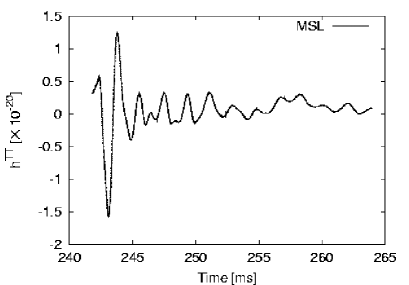
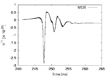
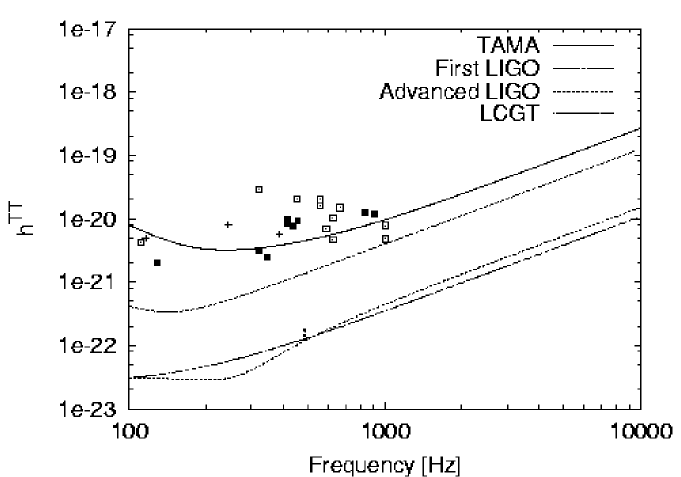
They also discussed the relation between the maximum amplitudes of gravitational wave and the initial $T/|W|$, which is the ratio of the rotational to the gravitational energy. From Figure 117, it was found that the largest amplitude is obtained for the moderate initial rotation rate (i.e., $T/|W|_{\rm init}=0.5\%$) when one fixes the initial rotation law and the degree of differential rotation. This is understood as follows. The amplitude of gravitational wave is roughly proportional to the inverse square of the typical dynamical scale, $t_{\rm dyn}$. Since $t_{\rm dyn}$ is proportional to the inverse square root of the central density $\rho$, the amplitude is proportional to the density. As a result, the amplitude becomes smaller as the initial rotation rates become larger because the density decreases then. On the other hand, the amplitude is proportional to the quadrupole moment, which becomes larger in turn as the total angular momentum increases. This is because stronger centrifugal forces not only make the mass of the inner core larger, but also deform it. The amplitude of gravitational wave is determined by the competition of these factors. As a result, the amplitudes is found to become maximal for moderate initial rotation rates. This is also noticed by the earlier work by Yamada and Sato (1995) [367].

Figure 117: Relations between $T/|W|_{\rm init}$ and the peak amplitude $|h^{\rm TT}|_{\rm max}$ for all the models [174]. In the figure, “CS, SS, SL, CL seq” represent the model sequences whose initial rotation profiles differ (see [174] for details). Note that the distance of the source is assumed to be located at the distance of 10 kpc.

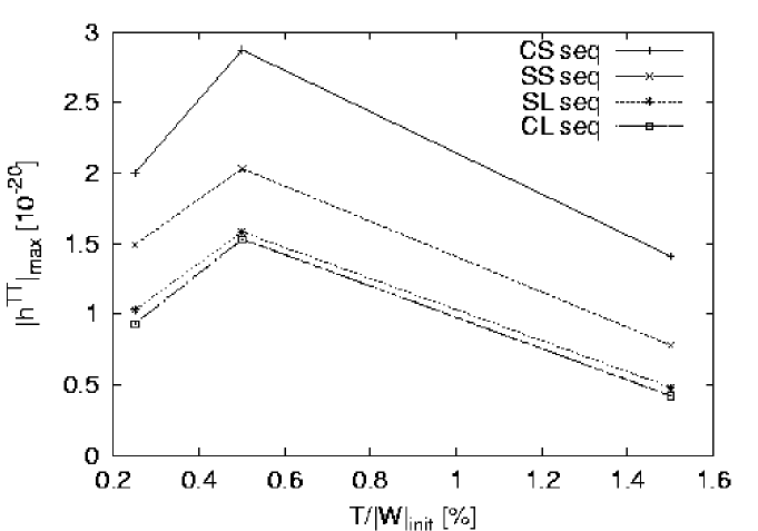
Combining the result by Finn [91], who pointed out by a perturbation technique that the amplitudes of the GWs are proportional to the square of the angular momentum $h\sim J^{2}$ in slowly rotating cases, the relation between the initial angular momentum and the peak amplitudes up to the rapidly rotating cases could be understood.

6.2.3 effects of magnetic fields

In addition to rotation discussed so far, Kotake et al (2004) investigated the effect of magnetic fields on the gravitational signals [179].

They extended the quadrupole formulae (Eq. (333)) in a form including the contributions from the electromagnetic fields. To begin with, $I^{20}$ in Eq. (360) should be replaced by $M_{20}^{\rm{E}2}$ as follows,

$$A_{20}^{\rm{E}2}=\frac{d^{2}}{dt^{2}}M_{20}^{\rm{E}2},$$ (367)

where the mass quadrupole formula is given as

$$M_{20}^{\rm{E}2}=\frac{G}{c^{4}}\frac{32\pi^{3/2}}{\sqrt{15}}\int_{0}^{1}d\mu\int_{0}^{\infty}dr~{}\rho_{*}\Bigl{(}\frac{3}{2}\mu^{2}-\frac{1}{2}\Bigr{)}r^{4},$$ (368)

where $\rho_{*}$ represents the total energy density including the contribution from the magnetic field,

$$\rho_{*}=\rho+\frac{B^{2}}{8\pi c^{2}}.$$ (369)

By a straightforward, however tedious, calculation to replace the time derivatives by the spatial derivatives applying the continuity equation, the equation of motion, and the induction equation,

$$\frac{\partial\mbox{\boldmath$B$}}{\partial t}=\nabla\times(\mbox{\boldmath$v$}\times\mbox{\boldmath$B$}),$$ (370)

noting the divergence-free constraint ($\nabla\cdot\mbox{\boldmath$B$}=0$), $A_{20}^{\rm{E}2}$ can be transformed into the following form,

$$A_{20}^{\rm{E}2}\equiv{A_{20}^{\rm{E}2}}_{\rm,quad}+{A_{20}^{\rm{E}2}}_{\rm,Mag},$$ (371)

where ${A_{20}^{\rm{E}2}}_{\rm,quad}$ is the contribution from the matter:

$${A_{20}^{\rm{E}2}}_{\rm,quad} = \frac{G}{c^{4}}\frac{32\pi^{3/2}}{\sqrt{15}}\Biggl{(}\int_{0}^{1}d\mu\int_{0}^{\infty}r^{2}\,dr\,\rho[{v_{r}}^{2}(3\mu^{2}-1)+{v_{\theta}}^{2}(2-3\mu^{2})-{v_{\phi}}^{2}-6v_{r}v_{\theta}$$ (372)

$$\,\mu\sqrt{1-\mu^{2}}-r\partial_{r}\Phi(3\mu^{2}-1)+3\partial_{\theta}\Phi\,\mu\sqrt{1-\mu^{2}}]-$$

$$\int_{0}^{1}d\mu\int_{0}^{\infty}r^{3}\,dr[q_{r}(3\mu^{2}-1)-3~{}q_{\theta}~{}\mu\sqrt{1-\mu^{2}}]\Biggr{)},$$

${A_{20}^{\rm{E}2}}_{\rm Mag}\equiv{A_{20}^{\rm{E}2}}_{j\times B}+{A_{20}^{\rm{E}2}}_{\rho_{\rm m}}$ is the contribution from the magnetic field:

$${A_{20}^{\rm{E}2}}_{j\times B} = \frac{G}{c^{4}}\frac{32\pi^{3/2}}{\sqrt{15}}\int_{0}^{1}d\mu\int_{0}^{\infty}r^{3}\,dr\Bigl{[}(3\mu^{2}-1)~{}\frac{1}{c}~{}(\mbox{\boldmath$j$}\times\mbox{\boldmath$B$})_{r}-$$ (373)

$$3\mu\sqrt{1-\mu^{2}}~{}\frac{1}{c}~{}(\mbox{\boldmath$j$}\times\mbox{\boldmath$B$})_{\theta}\Bigl{]},$$

$${A_{20}^{\rm{E}2}}_{\rho_{\rm m}} = \frac{G}{c^{4}}\frac{32\pi^{3/2}}{\sqrt{15}}\int_{0}^{1}d\mu\int_{0}^{\infty}\,dr~{}\frac{1}{8\pi c}$$ (374)

$$\frac{d}{dt}\Biggl{[}\frac{\partial}{\partial\theta}[B_{r}r^{3}(3~{}\mu^{2}-1)]E_{\phi}-\frac{\partial}{\partial r}[B_{\theta}r^{3}(3\mu^{2}-1)]rE_{\phi}+$$

$$+ \frac{\partial}{\partial r}[B_{\phi}r^{3}(3\mu^{2}-1)]rE_{\theta}-\frac{1}{\sin\theta}\frac{\partial}{\partial\theta}[B_{\phi}\sin\theta r^{3}(3\mu^{2}-1)]E_{r}\Biggr{]}.$$

${A_{20}^{\rm{E}2}}_{j\times B},{A_{20}^{\rm{E}2}}_{\rho_{\rm m}}$ represent the contribution from ${j\times B}$ part and from the time derivatives of the energy density of electro-magnetic fields, respectively. Only the first time derivative of the magnetic fields is remained, because this is the leading order and the numerical treatments of the second time derivatives are formidable. Then the total gravitational amplitude can be written as follows,

$$h^{\rm TT}\equiv h^{\rm TT}_{\rm quad}+h^{\rm TT}_{j\times B}+h^{TT}_{\rho_{\rm m}},$$ (375)

where the quantities of the right hand of the equation are defined by Eqs. (359), (372), (373), and (374). Note that $q_{r}$ and $q_{\theta}$ in Eq. (372) represents the gravitational waves contributed from the artificial viscosity (see e.g., [237]). When one uses an artificial viscosity of von Neumann and Richtmyer, which is a most popular one, the concrete form of $q_{i}$ is,

$$q_{i}=\nabla_{i}~{}[l^{2}~{}\rho~{}(\nabla\cdot\mbox{\boldmath$v$})^{2}],$$ (376)

where $i=r,\theta$ with $l$ defining the dissipation length. Using above quadrupole formula including contributions from the electromagnetic fields [368, 179], they calculated the waveforms by performing the 2D magnetohydrodynamic core-collapse simulations [179].

With these computations, they found that the amplitude is affected in the strongly magnetized models whose initial $E_{\rm m}/|W|$ is greater than 0.1 %, where $E_{\rm m}/|W|$ represents the magnetic to the gravitational energy. This is natural because the amplitude contributed from the electromagnetic fields should be an order of

$$R_{\rm mag}=\frac{{B_{\rm c}^{2}}/{8\pi}}{\rho_{\rm c}c^{2}}\sim~{}10~{}\%~{}\Bigl{(}\frac{B_{\rm c}}{\rm{several}~{}\times 10^{17}~{}\rm{G}}\Bigr{)}^{2}\Bigl{(}\frac{\rho_{\rm c}}{10^{13}~{}\rm{g}~{}\rm{cm}^{-3}}\Bigr{)}^{-1},$$ (377)

with $B_{\rm c},\rho_{\rm c}$ being the central magnetic field and the central density near core bounce, respectively. Thus, strongly magnetized models, whose central magnetic fields at core bounce become as high as $\sim 10^{17}$ G, can affect the amplitude.

Figure 118: Waveforms for a model with the strongest magnetic field obtained in the magnetohydrodynamic core-collapse simulation [179]. In the figure, “quad”,”$j\times B$” represent the contributions from the mass quadrupole moment and from the electromagnetic field, respectively (see Eq. (375)). The total amplitude is denoted as “tot”. Note that the source is assumed to be located at the distance of 10 kpc.

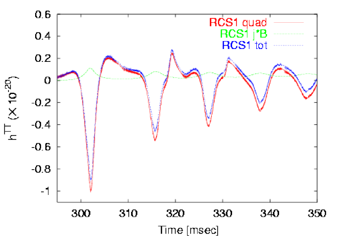
It was furthermore found that the contribution of the electromagnetic fields changes in the opposite phase to the matter contribution (see Figure 118). Together with a slight offset of the electromagnetic part, the negative part of the amplitude becomes less negative, while the positive part becomes more positive (see Figure 118). As a result, the peak amplitude at core bounce is found to be lowered by $\sim 10$ % They confirmed that the amplitudes of second peaks and the difference of its sign, from which one may know the information of the angular momentum of the core as mentioned, are still within the detection limit of the first LIGO for the galactic supernova, although the characteristics of second peaks are reduced by the incursion of the strong magnetic fields.

6.2.4 effects of realistic equations of state

We turn to the effect of the equation of state (EOS) on the gravitational signals. Needless to say, EOS is an important microphysical ingredient for determining the dynamics of core collapse and, eventually, the gravitational wave amplitude. As a realistic EOS, Lattimer-Swesty (LS) EOS [187] has been used in recent papers discussing gravitational radiations from the rotational core collapse [258, 242]. It has been difficult to investigate the effect of EOS’s on the gravitational signals because available EOS’s based on different nuclear models are limited. Recently, a new complete EOS for supernova simulations has become available [287, 303]. The EOS is based on the relativistic mean field (RMF) theory combined with the Thomas-Fermi approach.

By implementing these two realistic EOS’s, Kotake et al. (2004) looked into the difference of the gravitational wave signals [179]. The left panel of Figure 119 shows the waveforms for the models with the relativistic EOS (model MSL4) or the LS EOS (model MSL4-LS). The maximum amplitudes for the two models do not differ significantly (see the left panel of Figure 119). The important difference of the two EOS’s is the stiffness. As seen from the right panel of Figure 119, LS EOS is softer than the relativistic EOS, which makes the central density larger at core bounce and thus results in the shorter time interval between the subsequent bounces. On the other hands, softer EOS results in the smaller lepton fraction in the inner core, which reduces the mass quadrupole moments at core bounce. By the competition of these factors (see Eq. (365)), the maximum amplitude remains almost the same between the two realistic EOS’s, while the typical frequencies of the gravitational wave become slightly higher for the softer equation of state. Furthermore it was found that the aforementioned type III waveform observed in a very soft EOS polytropic equation of state [372] does not appear when the realistic equations of state are employed.

Figure 119: Waveforms (left panel) for the models with the relativistic EOS (the solid line labeled as MSL4) and with LS EOS (the dashed line labeled as MSL4-LS) and the relation between the central density and the effective adiabatic index $\gamma$ near core bounce (right panel).These figures are taken from [179].

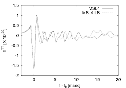
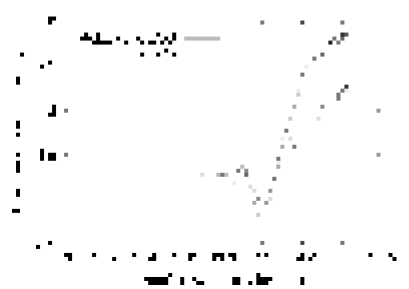
6.2.5 non-axisymmetric simulations

In addition to the above 2D simulations, several 3D simulations have been computed. The first 3D hydrodynamic core-collapse simulations well beyond the core bounce was performed by [263]. The initial condition for their study was based on the configuration at several milliseconds before core bounce in the rapidly rotating 2D models of Zwerger et al [372]. In addition to the configuration, they imposed low mode ($m=3$) density perturbation and followed the growth of the instability, where $m$ denotes the azimuthal quantum number. They observed the three clumps merged into a bar-like structure due to the growth of the non-axisymmetric instability (see the left panel of Figure 120). In fact, their models are rapid rotator whose value of $T/|W|$ at core bounce exceeds the critical value, beyond which MacLaurin spheroids become dynamically unstable against tri-axial perturbations ($T/|W|>T/|W|_{\rm dyn}\simeq 27.0\%$). However, they found that the maximum amplitudes of the gravitational waves were only $\sim 2\%$ different from the 2D cases by Zwerger et al.[372] (see the right panel of Figure 120).

Figure 120: Gravitational radiation in a 3D model taken from [263]. Left panels shows the contour of density in the equatorial plane after about 3 msec after core-bounce showing the growth of the three arms. From the left panel, it can be seen that the difference of gravitational amplitudes between the 3D models (dashed and dashed-dotted lines) and the axisymmetric models (solid line) at core-bounce (30 msec) are too small to see by eye. Cross mode of the gravitational waves $h_{\times}$, which is of genuine 3D origin begins to grow after core bounce ($t\geq 33$ msec), however, does not grow later on. (see [263] for details).

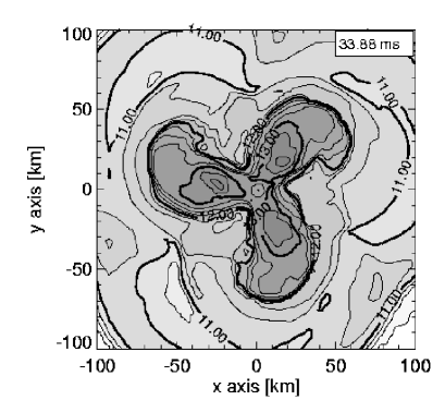
3D rotational core-collapse simulations of Fryer and his collaborators [101, 102] seem in favor of the above result. They have investigated whether the core fragmentation, and thus, the significant deviations of the gravitational radiation from 2D studies happen or not. As for the numerical computations, they have performed 3D smoothed particle hydrodynamic (SPH) simulations, with a realistic equation of state and the flux-limited diffusion approximation method for neutrino transfer. As for the initial model, they employed an rapidly rotating model with the initial value of $T/|W|_{\rm initial}$ of $\sim 3$ %. As a result, they also found that no fragmentation, although near core bounce the value of $T/|W|$ approaches to a critical value of $\sim$14 %, beyond which the secular instability due to the non-axisymmetric perturbations sets in. Since the maximum value of $T/|W|_{\rm initial}$ predicted by the recent evolution models are $\leq\sim 0.5\%$ [120], they concluded that the fragmentation or dynamical bar instabilities are unlikely to occur with any of the currently-produced supernova progenitors.

While the past studies terminated the 3D simulations at several tens milliseconds after core bounce, Ott et al (2005) investigated the growth of the non-axisymmetric structure until the rather later phases ($\geq 100$ msec) after core bounce [259]. They found that the growth of the $m=1$ mode, the so-called one-armed instability [65, 288, 289, 276], precedes the growth of the bar-mode ($m=2$) instability (see Figure 121), where $m$ denotes the azimuthal quantum number. Since the criterion of the growth of the one-armed instability is lower than that of the bar-mode instability [65, 288, 289, 276], they pointed out that the initial rotation rate required for the sufficient gravitational radiation from a galactic supernova enough to be detected by the future detectors can be as small as $T/|W|_{init}=0.2\%$, which is much smaller than the one previously assumed for igniting the growth of the bar-mode instability.

Figure 121: Time evolution of various quantities in a 3D model with $T/|W|_{\rm init}=0.2\%$ calculated by Ott et al. (2005) [259]. Time is measured from the epoch of core bounce $t_{b}$. Top panel shows that the amplitude of the $m=1$ mode precedes that of the $m=2$. Middle panel shows the time evolution of $T/|W|$ and the core’s maximum density. It is shown from the panel that after the epoch of $t-t_{b}\sim 100$ ms, when the $m=2$ mode begins to be amplified, the transfer of the angular momentum becomes active which results in the increase of the maximum density and the decrease of the $T/|W|$. The bottom panel shows the gravitational strain at the distance to the source $r$ as viewed down the rotational axis (solid curve) and as viewed along the equatorial plane (dotted curve). One can see that the waveform traces the time evolution of the $m=2$ mode. Note in the panel that $rh=100$ cm corresponds to $h\sim 3\times 10^{-21}$ for a galactic supernova.

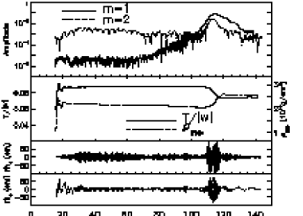
6.2.6 general relativistic studies

Figure 122:  Prospects of detection of the gravitational wave signal from axisymmetric rotational supernova core collapse in relativistic (black filled circles) and Newtonian (red unfilled circles) gravity studied in Dimmelmeier et al [79]. The figure gives the (dimensionless) gravitational wave amplitude $h^{\rm TT}$ and the frequency range for all 26 models. For a source at a distance of 10 kpc the signals of all models are above the burst sensitivity of the LIGO I detector (except for some low amplitude, high frequency models), and well above that of the LIGO II interferometer. It can be seen that the typical frequencies of the gravitational waves are blue-shifted when relativistic effects are taken into account. This figure is taken from Dimmelmeier et al [79].

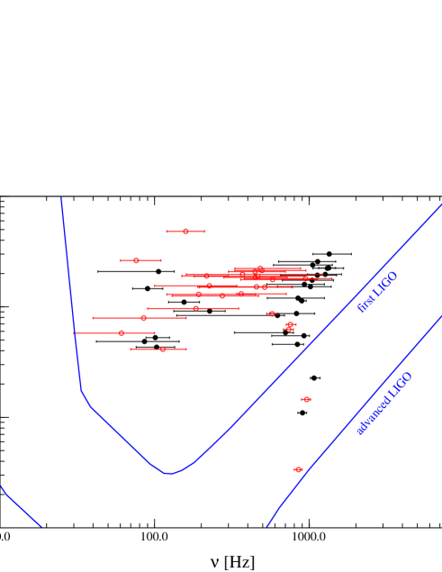
All the above computations employ the Newton gravity. In the following, we give a brief description of general relativistic (GR) studies. The study by [79] may be one of the representative GR studies for computing the GWs in stellar-collapse in the sense that they compared the properties of the GWs obtained by Newtonian and GR simulations systematically. As in the work of [372], they characterized the model difference by the degree of differential rotation, initial rotation rates, and adiabatic indices of equation of state and computed 26 initial models. The conformally flat (CF) metric was used to approximate the space time geometry in their GR hydrodynamic simulations. As well known, the CF approximation gives the exact solution of Einstein’s equation in spherical symmetry. The approximation may not be so bad unless the configurations are extremely deviated from the spherical symmetry. However, they were forced to employ the quadrupole formula for extracting the GWs because CF approximation eliminates the GW emission from the spacetime. With these computations, it was found that the qualitative features of the GWs obtained in the Newtonian studies of [372] are almost true for their studies. Quantitatively, however, it was pointed out that relativistic effects make the central density at core bounce much higher than that in the Newtonian gravity. This is simply due to the enhancement of the gravity due to the GR effect. As for the peak amplitudes at core bounce, no significant differences between the GR and Newtonian case were found, while the typical frequencies at the peak amplitudes are blue-shifted for the GR models. This may be because the higher central density makes the timescale at core bounce shorter, which leads to the higher frequency (see Figure 122).

Fully general relativistic collapse simulations from core-collapse to the formation of a neutron star have been performed by the group of M. Shibata [290] (see the reference, therein). It is mentioned that not only in their studies but also in other GR studies, the polytropic equations of state are employed in order to reduce the computational costs required for including a realistic equation of state. With these computations, it was found that not only the evolution of central density during core-collapse, bounce, and the formation of PNS, but also the waveforms are qualitatively in good agreement with those in the study of [79], except for a factor of $\sim$ 2 difference of the amplitudes in the ring-down phase (see Figure 123).

Figure 123: Comparison of the waveforms between the fully general relativistic (solid line) and conformally flat approximation (dotted line) calculations. This figure is taken from Shibata and Sekiguchi (2004) [290] .

As a result, they concluded that the approximated method by [79] is appropriate for following the axisymmetric stellar core-collapse associated with the formation of the neutron stars and for estimating the emitted gravitational waves. Needless to say, the full GR calculations are indispensable for estimating the gravitational waves from the core-collapse of very massive stars associated with the formation of the black hole.

Figure 124: Results of the first 3D full GR calculations taken from Shibata and Sekiguchi (2005) [291]. Left panel shows the gravitational waveform of the model with $T/|W|_{\rm init}\sim 1.8\%$ with the strong differential rotation (model M7c2 in [291]). $R_{+,\times}$ is the amplitude computed by the gauge-invariant extraction method, and $A_{+,\times}$ is the one by the quadrupole formula (see [291] for details). Right panel shows the snapshot of the contour of the density on the equatorial plane at $t=90.7$ ms with the vector fields (arrows), showing the bar-mode instability does develop, leading to the significant change in the amplitudes near the corresponding time. The maximum amplitude in the right panel can be translated into a dimensionless strain of $h\sim 10^{-18}$ for a galactic supernova with frequencies about 1 kHz.

The numerics of the general relativistic studies have seen major progress recently. Dimmelmeier et al. recently succeeded in extending their 2D GR code to 3D with the CF approximation [80]. Shibata and Sekiguchi (2005) have performed the fully general relativistic 3D simulations and pointed out that the amplitudes of the gravitational waves can be enhanced by a factor of $10$ than the axisymmetric collapse due to the growth of the dynamical bar-mode instabilities, when the core initially rotates very differentially with rapid rotation of $1\%\leq T/|W|_{\rm init}\leq 2\%$ [291] (see Figure 124). They discussed that the enhancement of the self-gravity due to the general relativistic effects results in a more efficient spin-up of the core, and thus, leading to the growth of the instability, which would be underestimated in the study of Rampp et al mentioned above. Very recently, fully general relativistic and magnetohydrodynamic simulations have also been reported to be practicable [81, 83]. The vary wide varieties of relativistic astrophysical events are expected to be investigated by the new-coming 3D GR studies.

6.3 Gravitational waves from convection and anisotropic neutrino radiation

All the studies, which we reviewed so far, paid attention to the gravitational signals produced near core bounce due to the large-scale aspherical motions of matter induced by core’s rotation without/with magnetic fields. In addition, two other sources of the GW emissions have been considered to be important in the later phases after core bounce, namely convective motions and anisotropic neutrino radiation, both of which can contribute to the non-spherical part of the energy momentum tensor of the Einstein equations. While gravitational waves from convective motions are originated from the aspherical motions of matter as well as the ones at core bounce, gravitational waves from neutrinos have some different features, which will be explained in the next section.

6.3.1 foundation of gravitational waves from neutrinos

As mentioned, the gravitational-wave signals at core bounce are emitted as bursts in which the wave amplitude rises from zero at core bounce, oscillates for several cycles and then approaches to zero (see for example Figure 114) due to the hydrodynamic motions of the central core. In addition, there is another class of gravitational wave, that is, bursts with memory, in which the wave amplitude rises from zero and then after the neutrino bursts settles into a non-zero final value [42]. The gravitational waves from anisotropic neutrino radiation from core-collapse supernovae is categorized to this class, which has been originately pointed out in late 1970’s by [87, 335]. The detectability of such effect was discussed by [42] through the ground-based laser interferometers. According to [87], we summarize the formulation of gravitational waves from neutrinos in the following, which will be useful in the later discussions.

At first, one should define a concrete form of an energy-momentum tensor of the neutrino radiation field to compute the gravitational waves. Then the following form is naturally assumed,

$$T^{ij}(t,\mbox{\boldmath$x$})=n^{i}n^{j}r^{-2}L_{\nu}(t-r)f(\Omega,t-r),$$ (378)

where $\mbox{\boldmath$n$}=\mbox{\boldmath$x$}/r,~{}r=|\mbox{\boldmath$x$}|,~{}f(\Omega,t)\geq 0,$ and $\int f(\Omega,t)d\Omega=1$. This source tensor represents radiation fields of neutrinos being released at the speed of light from the point $\mbox{\boldmath$x$}=0$ to an observer at a distance of $r$. The functions $L_{\nu}(t)$ and $f(\Omega,t)$ are the rate of energy loss and the angular distribution of neutrino radiation, respectively, at time $t$. Given the energy-momentum tensor, one can calculate the transverse-traceless (TT) gravitational field from the corresponding source as follows,

$$h_{\nu,TT}^{ij}=4\int T_{TT}^{ij}(t-|\mbox{\boldmath$x$}-\mbox{\boldmath$x$}^{{}^{\prime}}|,\mbox{\boldmath$x$}^{{}^{\prime}})|\mbox{\boldmath$x$}-\mbox{\boldmath$x$}^{{}^{\prime}}|^{-1}~{}d^{3}x^{{}^{\prime}}$$ (379)

Note that dashed $(^{{}^{\prime}})$ variables represent the quantities observed in a coordinate frame $(x^{{}^{\prime}},~{}y^{{}^{\prime}},~{}z^{{}^{\prime}})$, on the other hand, non-dashed variables represent the quantities observed in the observer’s frame $(x,~{}y,~{}z)$ (see Figure 125).

Figure 125: Source coordinate system $(x^{{}^{\prime}},y^{{}^{\prime}},z^{{}^{\prime}})$ and observer coordinate system $(x,y,z)$. The observer resides at the distant point on the $z$-axis. The viewing angle is denoted by $\xi$ which is the angle between $z$ and $z^{{}^{\prime}}$ axis. The $z^{{}^{\prime}}$ axis coincides with the symmetry axis of the source, presumably the rotational axis. Central red region indicates the anisotropic neutrino radiation from a supernova.

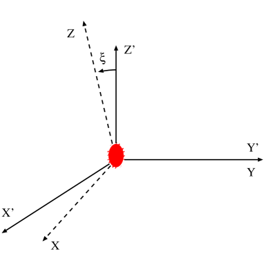
For convenience, we write Eq. (378) as follows,

$$T^{ij}(t,\mbox{\boldmath$x$})=n^{i}n^{j}r^{-2}\int_{-\infty}^{\infty}L_{\nu}(t^{{}^{\prime}})f(\Omega^{{}^{\prime}},t^{{}^{\prime}})~{}\delta(t-t^{{}^{\prime}}-r)dt^{{}^{\prime}}.$$ (380)

Introducing Eq. (378) to (379) and performing the integration with respect to $r^{{}^{\prime}}$ and we may obtain,

$$h^{ij}_{\nu,TT}(t,\mbox{\boldmath$x$})=4\int_{-\infty}^{t-r}\int_{4\pi}\frac{(n^{i}n^{j})_{TT}L_{\nu}(t^{{}^{\prime}})f(\Omega^{{}^{\prime}},t^{{}^{\prime}})}{t-t^{{}^{\prime}}-r\cos\theta^{{}^{\prime}}}d\Omega^{{}^{\prime}}~{}dt^{{}^{\prime}}.$$ (381)

In addition, we make use of the approximation that the gravitational wave signal measured by an observer at time $t$ is caused by radiation emitted at time $t^{{}^{\prime}}=t-r$. Hence we take $t-t^{{}^{\prime}}=const=r$, which means that only a neutrino pulse itself is assumed to cause a gravitational wave signal. This procedure is equivalent to eliminate the non-zero value of $h_{\nu}$ in case of isotropic neutrino radiation appeared in Eq. (381). We verify this in the later section.

In the geometrical setup shown in Figure 125, we assume that the $z$-axis lies on the ($x^{{}^{\prime}},z^{{}^{\prime}}$) plane for convenience. In this case, the two polarization states of gravitational waves satisfying the transverse-traceless conditions become

$$h^{+}_{\nu,\rm TT}\equiv h^{xx}_{\nu}=-h^{yy}_{\nu},$$ (382)

and

$$h^{\times}_{\nu,\rm TT}\equiv h^{xy}_{\nu}=h^{yx}_{\nu},$$ (383)

in the observer coordinates. It is noted that the sum of the squared amplitudes $|h_{+}|^{2}+|h_{\times}|^{2}$ is invariant under the rotation about the $z$-axis. Using the following relations between the two coordinates,

$$\sin\theta^{{}^{\prime}}\cos\phi^{{}^{\prime}}=\sin\theta\cos\phi\cos\xi+\cos\theta\sin\xi,$$ (384)

$$\sin\theta^{{}^{\prime}}\sin\phi^{{}^{\prime}}=\sin\theta\sin\phi,$$ (385)

$$\cos\theta^{{}^{\prime}}=-\sin\theta\cos\phi\sin\xi+\cos\theta\cos\xi,$$ (386)

one can obtain the following,

$$h_{\nu,+}^{\rm TT}=\frac{2}{r}\int_{-\infty}^{t-\frac{R}{c}}dt^{{}^{\prime}}\int_{4\pi}d\Omega^{{}^{\prime}}(1+\cos\theta)~{}\cos 2\phi~{}L_{\nu}(t^{{}^{\prime}})f(\Omega^{{}^{\prime}},t^{{}^{\prime}}),$$ (387)

while the counter part of the amplitude, $h_{\times}$, is obtained just replacing $\cos 2\phi$ with $\sin 2\phi$, which immediately becomes zero by integrating over the angle $\phi$ due to the axisymmetric source we consider here.

In the above equation, it should be noted that $\theta$ and $\phi$ are required to be expressed in terms of the angles $\vartheta^{{}^{\prime}},~{}\phi^{{}^{\prime}}$ with respect to the source coordinate valuables, and the viewing angle of $\xi$. In the following, we consider two cases, in which the observer is situated parallel to the $z^{{}^{\prime}}$ axis ($\xi=0$) or perpendicular to the $z^{{}^{\prime}}$ axis ($\xi=\pi/2$). In the former case, one easily obtains,

$$h_{\nu,\rm p}^{\rm TT}=\frac{2}{r}\int_{-\infty}^{t-\frac{R}{c}}dt^{{}^{\prime}}\int_{4\pi}d\Omega^{{}^{\prime}}(1+\cos\vartheta^{{}^{\prime}})~{}\cos 2\varphi^{{}^{\prime}}~{}L_{\nu}(t^{{}^{\prime}})f(\Omega^{{}^{\prime}},t^{{}^{\prime}}),$$ (388)

which becomes zero in case of the axisymmetric radiation source. Here the subscript _p suggests that the observer is situated in the polar axis relative to the source coordinate frame. In the latter case, the observer is positioned perpendicular to the source’s $z^{{}^{\prime}}$ axis (seen from the $e$quator), and the field becomes,

$$h_{\nu,\rm e}^{\rm TT}=\frac{2}{r}\int_{-\infty}^{t-\frac{R}{c}}dt^{{}^{\prime}}\int_{4\pi}d\Omega^{{}^{\prime}}\Psi(\vartheta^{{}^{\prime}},\varphi^{{}^{\prime}})~{}L_{\nu}(t^{{}^{\prime}})f(\Omega^{{}^{\prime}},t^{{}^{\prime}}),$$ (389)

where,

$$\Psi({\vartheta^{{}^{\prime}},\varphi^{{}^{\prime}}}) = (1+\sin\vartheta^{{}^{\prime}}\cos\varphi^{{}^{\prime}})\frac{\cos^{2}\vartheta^{{}^{\prime}}-\sin^{2}\vartheta^{{}^{\prime}}\sin^{2}\varphi^{{}^{\prime}}}{\cos^{2}\vartheta^{{}^{\prime}}+\sin^{2}\vartheta^{{}^{\prime}}\sin^{2}\varphi^{{}^{\prime}}}.$$ (390)

Since the amplitudes from neutrinos become largest seen from the equatorial plane of the source, we regard the Eq. (389) as the base formula to compute the amplitudes from neutrinos. we use the gravitational waves from neutrinos are anti-beaming

Next, we make an order-of-magnitude estimate of the amplitude of the gravitational waves for neutrinos [87, 241]. From Eq. (389), one can estimate the amplitudes, $h_{\nu}$, as follows,

$$h_{\nu}=\frac{2G}{c^{4}D}\int_{-\infty}^{t-R/c}dt~{}L_{\nu}(t^{{}^{\prime}})\cdot\alpha(t^{\prime}),$$ (391)

where $D$ is the distance to the source and $\alpha(t^{{}^{\prime}})$ is the time-dependent anisotropy parameter,

$$\alpha(t^{{}^{\prime}})=\int_{4\pi}d\Omega^{{}^{\prime}}\Psi(\vartheta^{{}^{\prime}},\varphi^{{}^{\prime}})~{}f(\Omega^{{}^{\prime}},t^{{}^{\prime}}),$$ (392)

representing the degree of the deviation of the neutrino emission from spherical symmetry. Inserting typical values into the above equation, one can find the typical amplitudes,

$$h_{\nu}\sim 1.6\times 10^{2}{\rm cm}~{}\frac{1}{D}\Bigl{(}\frac{\alpha}{0.1}\Bigr{)}\Bigl{(}\frac{L_{\nu}}{10^{52}~{}{\rm erg}~{}{\rm s}^{-1}}\Bigr{)}\Bigl{(}\frac{\Delta t}{1~{}{\rm s}}\Bigr{)},$$ (393)

where we take an emission time of $\Delta t=1$ s assuming constant radiation and the optimistic values of $\alpha\sim 0.1$ suggested from the numerical results [241]. Thus it is expected that the gravitational-wave amplitude from neutrinos can be larger than the one emitted at core bounce in rotational core-collapse (see Eq. (365)). The typical frequency of the gravitational waves from neutrinos is expected to be lower by an order of magnitude than the one at the core bounce in rotational-core collapse, because the dynamical scale is not determined at the central core $\rho\sim 10^{14}~{}{\rm g}~{}{\rm cm}^{-3}$ but at the neutrinosphere $\rho\sim 10^{12}~{}{\rm g}~{}{\rm cm}^{-3}$.

It is noted that the gravitational memory stems from the change in the transverse-traceless part of the Coulomb-type ($\propto 1/r$), and thus, can appear in other astrophysical events. Recently, the memory effect generated by a point particle whose velocity changes via gravitational interactions with other objects is studied [277]. Further, the memory in the context of jets in gamma-ray bursts is studied, which predicts that such gravitational waves are likely to be detected by the space-based laser interferometers such as LISA and DECIGO/BBO [275, 135].

Now we return to mention the gravitational waves from neutrinos and convections from core-collapse supernovae in the following sections.

6.3.2 gravitational waves from convections and neutrinos in non-rotating stars

As mentioned in section 5.3, the convections are likely to occur in the protoneutron stars and in the hot bubbles regions. In Figure 126, a typical GW waveform due to the convective motions and the associated anisotropic neutrino radiation inside the non-rotating protoneutron star (PNS) is presented. From the left panel, the time interval of the each GW signal from convections (thick line) is found to be very short with an order of milliseconds, while the waveform associated with the neutrinos (thin line) shows much less time structure. The short interval of the GWs from matter reflects the timescale of the convective motion inside the PNS, which may be roughly estimated as follows, $t_{\rm conv}\leq\sim R_{\rm PNS}/v_{\rm conv}\sim{O\rm(ms)}~{}(R_{\rm PNS}/20{\rm km})/(v_{\rm conv}/1\times 10^{9}~{}{\rm cm}~{}{\rm s}^{-1})$ with $R_{\rm PNS}$ and $v_{\rm conv}$ being the size of the PNS and the typical velocity of the convective motions. Since the amplitudes both from matter and neutrinos result from the small-scale motions induced mainly by the negative gradient of the lepton fraction, the amplitudes become much smaller than the ones at core bounce in rotational core-collapse (typically $\leq 1/10$). Due to the smaller amplitudes and the higher frequencies of the emitted gravitational waves, both unlike the ones obtained at core bounce in rotational core-collapse, they are marginally within the detection limits for the laser interferometer in the next generation (see the right panel of Figure 126).

Figure 126: Computations of the gravitational wave in the non-rotating protoneutron star (PNS) taken from [242]. The left panel shows the waveform due to the convective motion (thick line labeled as “flow”) and the anisotropic neutrino radiation (thin line labeled as “$\nu^{\prime}{\rm s}$”). The insert shows an enlargement of the signal until $\sim 100$ ms from the start of the simulation. The right panel shows the total gravitational spectrum with the sensitivity curves for some detectors. The source is located at a distance of 10 kpc. These figures are taken from Müller et al (2003) [242].

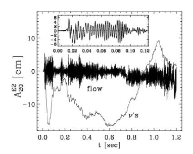
Not only inside the PNS, but also outside the PNS, the convections are likely to be induced, as stated earlier (see section 5.3). Burrows & Hayes (1996) [51] performed 2D simulations, in which the density of the precollapse core was artificially reduced 15 % within $20$ degree of the pole, and demonstrated how the initial density inhomogeneity affects the gravitational waves both from the convective motions and the anisotropic neutrino radiation. The large density inhomogeneity assumed in their work was predicted by the stellar evolution calculations, pointing out that they could be formed and amplified during silicon and oxygen burning stages [31, 112]. The obtained properties of the waveform is presented in Figure 127. They discussed that the total amplitude could be detected by the advanced LIGO, with a signal-to-noise ratio of 10, for a supernovae at a distance of 10 kpc.

With almost the same motivation for the investigation, Fryer et al performed 3D SPH simulations of the inhomogeneous core-collapse and discussed the waveforms [101, 102].

Figure 127: The gravitational wave strain, $h_{\rm zz}^{TT}$ times the distance to the supernova, D, versus time. Core bounce is at 0,215 seconds. Each line shows the corresponding contributions to the gravitational waves. The contributions of matter motion and neutrinos to the GW amplitude can be seen of opposite sign at core bounce. Only for the first 20 ms after core bounce, the gravitational waves from neutrinos are shown to dominate over the mass motions. This figure is taken from Burrows & Hayes [51].

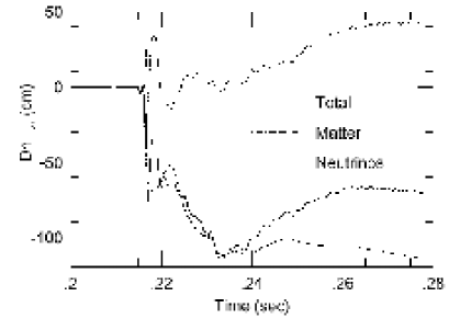
The computed signatures of the gravitational waves are consistent with the study of [51]. They discussed that such gravitational waves are within the detection limits for the advanced LIGO for the galactic supernova (see Figure 128). As shown by the simple order-of-magnitude estimates (Eq. (393)), it is seen from the right panel that the peak amplitude form neutrinos becomes as high as the one at core bounce ($h\sim 10^{-20}$) with the relatively lower peak frequency.

Figure 128: Gravitational from anisotropic neutrino radiation as a function of time and observer location (left) and its spectrum (right), obtained in the 3D simulations [103]. In the model, a 25 $\%$ core oscillation perturbation is assumed in the iron core of $15M_{\odot}$ progenitor star for producing the asphericity of the neutrino radiation field. From the right panel, it can be seen that the gravitational wave from the neutrinos peaks at lower frequencies and within the detection limits for the Advanced LIGO for the galactic supernova at the distance of $10$ kpc. These figures are taken from Fryer et al [103].

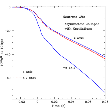
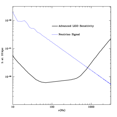
Both in the above studies of [51] and [101, 102], a large density inhomogeneity ($\sim O(10)\%$ fluctuations in the density) prior to core-collapse is assumed in their initial conditions. On the other hand, it is noted that a recent study pointed out by the linear stability analysis in the cores of supernova progenitor stars that the timescale for the growth of the nuclear burning (the so-called $\epsilon$ mechanism) is much longer than the time until the commencement of core-collapse, hence such a large inhomogeneity may not develop [233].

Figure 129: Computations of the GW in rotational core collapse obtained by the state-of-the-art simulations ($\Omega=0.5~{}{\rm rad}~{}{\rm s}^{-1}$ is imposed on $15M_{\odot}$ progenitor model) [242]. In the left panel the waveforms contributed from neutrinos and the matter flows are shown. It is shown that the gravitational waves from neutrinos dominate over the ones from the flows almost always. The middle panel shows the spectrum of gravitational waves contributed from neutrinos. The right panel shows the total gravitational spectrum with the sensitivity curves for some detectors. Comparing the middle with the right panel, one can see that the gravitational waves in the lower frequency ($\leq 100$ Hz) are dominated by the neutrinos. These figures are taken from Müller et al. (2003) [242].

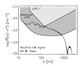
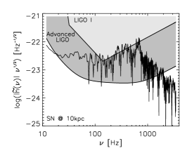
6.3.3 gravitational waves from anisotropic neutrino radiation in rotating stars

Another possibility to induce the anisotropy of neutrino emissions is the stellar rotation. Recently, Müller et al (2004) [242] performed the rotational core collapse simulations employing the elaborate neutrino transport with the detailed microphysics and calculated the gravitational waves from neutrinos. They found that the gravitational waves from the neutrinos grows due to convections and dominate over those of the matter at core bounce (see Figure 129).

In their study, the initial models were limited to the rather slower rotating cases based on a recent stellar evolution models, in which the magnetic braking is taken into account [121, 122]. Recently, Kotake et al (2005) [176] calculated the waveforms from neutrinos employing a series of more rapidly rotating models with changing the rotational profiles and the degree of differential rotation parametrically in order to see the effects of anisotropy of the neutrino radiation induced dominantly by rapid rotation.

Figure 130: Left panel is the waveform due to the anisotropic neutrino radiation for model S10. In the panel, points A, B, C, and D represents the epoch of core bounce ($t=242.7~{}{\rm ms}$), the onset of the first neutronization ($t=244.8~{}{\rm ms}$), the peak of the neutronization, which corresponds to the onset of the second neutronization ($t=245.3~{}{\rm ms}$), and the offset of the second neutronization ($t=246.1~{}{\rm ms}$), respectively. Right panel represents the angular dependence of $\Phi$ in Eq. (394). Note that the angle is measured from the rotational axis. These figures are taken from [176].

Figure 131: Waveforms due to the anisotropic neutrino radiations for some representative models with the shell-type (left panel) and the cylindrical rotation (right panel) profiles. Note that the source is assumed to be located at the distance of 10 kpc. These figures are taken from [176].

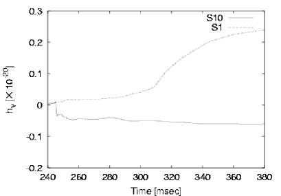
In the left panel of Figure 130, the waveform for a typical model studied in [176] near core bounce is given. Note that the model is based on the recent stellar evolution calculation while excluding the effects of the magnetic fields [120]. About 2.1 ms after core bounce at point A in the panel, the amplitude begins to rise more steeply than before (see point B in the figure). This epoch corresponds to the so-called neutronization, which occurs when the shock wave goes over the neutrino sphere. Here it should be noted that the neutronization occurs anisotropically in their rotating models. Due to the non-sphericity of the shapes of the shock wave and the neutrino sphere, the neutronization can occur more than once while it occurs only once for spherical models. In which direction the neutronization occurs is determined by the shapes of the deformed neutrino sphere and the anisotropically propagating shock wave. The first neutronization (at point B in the panel) occurs near the pole at the radius of $\sim 20~{}{\rm km}$ along the rotational axis. The shape of the shock wave formed by core bounce is prolate initially because the bounce occurs near the rotational axis. This prolate shock wave crosses the neutrino sphere, whose shape is deformed to be oblate due to rotation. Since the area of surface, where the first neutronization occurs, is small, the neutrino luminosity is relatively low at this epoch ($L_{\nu}\sim 10^{52}~{}\rm{erg}~{}\rm{s}^{-1}$). About 0.5 ms after the first neutronization at point B in the left panel of Figure 130, the amplitude shows sudden fall from $t=245.3$ ms (point C) to $t=246.1$ ms (point D). After the first neutronization occurs at the pole, the shock wave in the polar region is weakened by the neutrino energy loss and ram pressure of the infalling material. Then, the subsequent shock wave is formed in the vicinity of the equatorial plane and begins to move rather parallel to the plane. Since the first shock wave almost stalls along the rotational axis during a several millisecond after the first neutronization, the shape of the shock wave becomes rather oblate due to the propagation of the second shock wave rather parallel to the equatorial plane. As this oblate shock wave propagates along the equatorial plane, it crosses the oblate neutrino sphere. At this moment, the second neutronization occurs, where its luminosity becomes maximum, whose value reaches as high as $\lesssim 10^{54}{~{}\rm erg}~{}{\rm s}^{-1}$.

They explained the signatures of the gravitational waves at the two epochs of the neutronization as follows. At the first neutronization, the neutrino emissions are concentrated near the rotational axis. For convenience to understand the relation between the direction of neutrino emissions and the resultant properties of the waveforms, we analytically integrate over $\varphi^{{}^{\prime}}$ in Eq. (389) and obtain the formula in the closed form as follows,

$$h^{\rm TT}_{\nu}=\frac{8G}{c^{4}R}\int_{-\infty}^{t-R/c}dt^{{}^{\prime}}\int_{0}^{\pi/2}~{}d\theta^{{}^{\prime}}~{}\Phi(\theta^{{}^{\prime}})~{}\frac{dL_{\nu}(\theta^{{}^{\prime}},t^{{}^{\prime}})}{d\Omega^{{}^{\prime}}},$$ (394)

where $\Phi(\theta)$ is the latitudinal angle dependent function,

$$\Phi({\vartheta^{{}^{\prime}}}) = \sin\vartheta^{{}^{\prime}}\Bigl{(}-\pi+\int_{0}^{2\pi}d\varphi^{{}^{\prime}}\frac{1+\sin\vartheta^{{}^{\prime}}\cos\varphi^{{}^{\prime}}}{1+\tan^{2}\vartheta^{{}^{\prime}}\sin^{2}\varphi^{{}^{\prime}}}\Bigr{)},$$ (395)

(see the right panel of Figure 130) and ${dL_{\nu}(\theta,t)}/{d\Omega}$ is the latitudinal angle dependent neutrino luminosity. From the formula, one can readily see that no gravitational waves can be emitted if the neutrino emissions are spherical.

From the feature of $\Phi$ seen in the panel, the enhancement of the neutrino radiation near the rotational axis does not work sufficiently to change the amplitude although the amplitude shows a rise at the first neutronization due to the non-zero contributions of $\Phi$ and the neutrino luminosity near the rotational axis (see from point B to C in Figure 130). On the other hand, at the second neutronization, the neutrino emissions are concentrated in the vicinity of the equatorial plane. The value of the function $\Phi$ is negative ($\theta=\pi/2$) and its absolute value is large compared to the value near the rotational axis ($\theta\sim 0$) (see the right panel of Figure 130). In addition, the neutrino luminosity is much larger at the second neutronization. This is because the area of the surface at the second neutronization is quite larger than that at the first neutronization near the pole, since the oblate shock wave crosses the oblate neutrino sphere. As a result, the amplitude of the gravitational waves from the neutrinos shows a steep fall at the second neutronization.

Moreover they demonstrated that the differential rotation mainly determines the waveforms. In Figure 131, the waveforms $h_{\nu}$ from near core bounce up to the final time of their simulation are presented for the representative models with the shell-type (left panel) and cylindrical rotation profiles (right panel), respectively. It can be seen from the figures that the amplitude due to the neutrinos in the later times becomes much larger for the models with the stronger differential rotation (compare S10 (weakest differential rotation with initial angular velocity cut of $1000$ km) with S1 (strongest differential rotation with initial angular velocity cut of $100$ km), CS10 (weakest one) with CS1 (strongest one), respectively). Simultaneously, it is found that this feature is regardless of the rotational profiles (compare the left (shell-type rotation) with the right panels (cylindrical rotation) in Figure 131). As the differential rotation becomes stronger, the shape of the shock wave becomes more prolate, which makes the neutrino emission more stronger in the vicinity of the rotational axis. This makes the gravitational amplitudes from the neutrinos more larger (see [176] for the more detailed explanations).

Figure 132: Detection limits of TAMA, first LIGO, advanced LIGO, and Large-scale Cryogenic Gravitational wave Telescope (LCGT) with the expected gravitational wave spectrum obtained from the numerical simulations. The left panel shows the gravitational-wave spectrum contributed from neutrinos (solid) and from the matter (dashed) in a rotating model with $\Omega=4~{}{\rm rad}~{}{s}^{-1}$ imposed initially on a 15 $M_{\odot}$ progenitor model. In the right panel, the open circles and the pluses represent the amplitudes of $h_{\nu,{\rm eq}}$ with the characteristic frequencies of $\nu_{\rm eq}$ for the models with the cylindrical and the shell-type rotation profiles, respectively. Under the frequency of $\nu_{\rm eq}$, the gravitational waves from the neutrinos dominate over those from the matter contributions. From the panel, it is seen that the gravitational waves from neutrinos dominate over the ones from the matter in a lower frequency ($f\leq 100$ Hz). Note that the source is assumed to be located at the distance of 10 kpc. These figures are taken from [176].

In the left panel of Figures 132, the root mean square (rms) sensitivity curves with the rms gravitational wave spectra for the standard model is given. From the panel, it can be seen that the gravitational waves due to the anisotropic neutrino radiation dominate over those due to the mass motions at the frequency lower than several 10 Hz. In the 21 models computed, it is found that the values of $\nu_{\rm eq}$ ranges from 8 to 58.1 Hz with the rms amplitude ranging from $7.28\times 10^{-23}$ to $1.28\times 10^{-21}$ and that the values of $h_{\nu,\rm eq}$ generally become larger for the stronger differential rotation models. Here $\nu_{\rm eq}$ represents a characteristic frequency, below which the gravitational waves from the neutrinos dominate over those from the mass motions, and the corresponding rms gravitational wave amplitude is named as $h_{\nu,\rm eq}$. In the right panel of Figure 132, the values of $h_{\nu,\rm eq}$ with $\nu_{\rm eq}$ for all the models are plotted with the sensitivity curves of laser interferometers. It can be seen that the gravitational waves from the neutrinos are the detection limits of the detectors in the next generation such as LCGT and advanced LIGO. Thus, it is suggested that the detection of the gravitational wave at the low frequency range ($\lesssim 100$ Hz) becomes more hopeful due to the contributions from the anisotropic neutrino radiation.

7 Concluding Remarks

The aim of writing this article was to provide an overview of what we currently know about the explosion mechanism, neutrinos, and gravitational waves in core-collapse supernovae. As we have discussed, much progress has been made in each topics.

Recently, multidimensional studies and simulations of core-collapse supernovae have come into blossom again since 1990’s when the direct observations of global asymmetry in SN 1987A were reported. The current trend might be ascribed to the fact that spherically symmetric supernova simulations have not yet produced explosions, albeit with the probably “ultimate” sophistication of the neutrino-transport method including the state-of-the-art microphysics. A step beyond the spherical models is in steady progress. It seems most natural and convincing to investigate the effect of the asphericity on the neutrino heating mechanism. Many ingredients to produce asymmetry in the supernova core have been considered, e.g., stellar rotation, magnetic fields, convection, and the standing accretion shock instability. In order to see the real outcome of them, we should be able to perform at least two-dimensional fully angle-dependent radiation-hydrodynamic calculations. In fact, several groups are really pursuing it with the use of advanced numerical techniques.

Understanding the explosion mechanism of core-collapse supernovae is important not only for itself but also for the theoretical understanding for the other (astro)physical relevance, such as neutrino and gravitational-wave emissions. Conversely, we are now being able to understand them from the observations. In fact, neutrino and gravitational-wave astronomy are now becoming reality.

Neutrino is a powerful tool to probe deep inside of the supernova while we can see just its surface by electromagnetic waves. In fact, supernova gave the first stage for the Neutrino Astronomy when we observed neutrinos from SN1987A. Neutrinos reflect the physical state of the core and even the density structure of the mantle if we consider neutrino oscillation. Actually neutrino oscillation is a necessary physics when we want to extract information on supernova from observed neutrinos because neutrino oscillation changes the neutrino spectra. However, this cannot be done so easily because there are some ambiguities in one of neutrino oscillation parameters, $\theta_{13}$, and mass hierarchy, although we have other parameters with high accuracies. Conversely, this means that supernova can be a unique laboratory which probes the unknown neutrino parameters which can not be studied by other experiments such as solar, atmospheric, accelerator and reactor experiments.

Gravitational wave is also a powerful tool, which gives us the information deep inside the supernova core. If the supernova core rotates rapidly, the burst-like gravitational waves are emitted at core bounce, and their amplitudes are as strong as the currently running interferometric observatories could detect for a galactic supernova. While this is not the case, gravitational waves emitted in the later phase due to the convective motions and the anisotropic neutrino emissions will be most promising for the detections. Especially, the gravitational signal from neutrinos have different features from the other, in the sense that they have memory, the detection may need somewhat different technique. If we could detect the gravitational waves from anisotropic neutrino emissions simultaneously with neutrinos themselves, it will bring about the great progress in the understanding of the explosion mechanism, because the anisotropy should play a important role. Moreover, the mutual understanding of the explosion mechanism, the supernova neutrinos, and the gravitational waves, which we reviewed somewhat separately in this article, will be greatly progressed.

Moreover, supernova study is indispensable for the understanding of some hot astrophysical issues, such as the central engine of gamma-ray bursts and the nucleosynthesis in the explosion of population III stars. Further study will have a great impact not only on disclosing the mechanism of such astrophysical phenomena, but also on unveiling the fundamental properties of particle physics.

References

- [1] Achkar B et al 1995 Search for neutrino oscillations at 15, 40 and 95 meters from a nuclear power reactor at Bugey Nucl. Phys. B 434 503-532
- [2] Aglietta M et al 1992 THE MOST POWERFUL SCINTILLATOR SUPERNOVAE DETECTOR: LVD Il Nuovo Cimento A 105 1793-1804
- [3] Akhmedov E Kh et al 2002 Supernova neutrinos: difference of fluxes and conversion effects Nucl. Phys. B 643 339-366
- [4] Akiyama S et al 2003 The Magnetorotational Instability in Core-Collapse Supernova Explosions Astrophys. J. 584 954 - 70
- [5] Alekseev E N et al 1987 POSSIBLE DETECTION OF A NEUTRINO SIGNAL ON 23 FEBRUARY 1987 AT THE BAKSAN UNDERGROUND SCINTILLATION TELESCOPE OF THE INSTITUTE OF NUCLEAR RESEARCH JETP Lett. 45 589-592
- [6] AMANDA Collaboration, web page, http://amanda.wisc.edu/
- [7] AMANDA Collaboration 2002 Mod. Phys. Lett. A 17 2019
- [8] Ando M and TAMA collaboration 2002 Class. Quantum Grav. 19 1409
- [9] Ando S and Sato K 2002 Determining the Supernova Direction by its Neutrinos Prog. Theor. Phys. 107 957
- [10] Ando S 2003 Asymmetric neutrino emission due to neutrino-nucleon scatterings in supernova magnetic fields Phys. Rev. D 68 063002
- [11] Arafune J and Fukugita M 1987 PHYSICAL IMPLICATIONS OF THE KAMIOKA OBSERVATION OF NEUTRINOS FROM SUPERNOVA SN1987A.
- [12] Ardeljan N V et al 2000 Nonstationary magnetorotational processes in a rotating magnetized cloud Astron. Astrophys. 355 1181 - 90
- [13] Arnett W D 1983 Neutrino escape, nuclear dissociation, and core collapse and/or explosion Astrophys. J. 263 L55-L57 Phys. Rev. Lett. 59 367
- [14] Arnett W and Rosner J 1987 NEUTRINO MASS LIMITS FROM SN1987A Phys. Rev. Lett. 58 1906
- [15] Arras P and Lai D 1999 Can Parity Violation in Neutrino Transport Lead to Pulsar Kicks? Astrophys. J. 519 745 - 9
- [16] Arras P and Lai D 1999 Neutrino-nucleon interactions in magnetized neutron-star matter: The effects of parity violation Phys. Rev. D 60 043001-1 - 28
- [17] Arzoumanian Z et al 2002 The Velocity Distribution of Isolated Radio Pulsars Astrophys. J. 568 289 - 301
- [18] Baade W and Zwicky F 1934 Remarks on Super-Novae and Cosmic Rays Phys. Rev. 46 76-77
- [19] J. N. Bahcall, web page, http://www.sns.ias.edu/ jnb/
- [20] Bahcall J N 1989 Neutrino Astrophysics (Cambridge University Press).
- [21] Bahcall J N 2004 Solar Models and Solar Neutrinos: Current Status hep-ph/0412068
- [22] Bahcall J N et al 2005 Helioseismological Implications of Recent Solar Abundance Determinations Astrophys. J 618 1049-1056
- [23] Bahcall J N and Glashow S L 1987 UPPER LIMIT ON THE MASS OF THE ELECTRON-NEUTRINO Nature 326 476
- [24] Bahcall J N et al 2005 New solar opacities, abundances, helioseismology, and neutrino fluxes Astrophys. J 621 L85-L88
- [25] Bahcall J N et al SN1987A in The Large Magellanic Cloud, Proceedings of the Fourth George Mason Astronomy Workshop, Fairfax, Virginia, ed. M. Kafatos, (Cambridge Univ. Press), p. 172.
- [26] Balbus S A and Hawley J F 1998 Instability, turbulence, and enhanced transport in accretion disks Reviews of Modern Physics 70 1-53
- [27] Balbus S A and Hawley J F 1991 A powerful local shear instability in weakly magnetized disks. I - Linear analysis. II - Nonlinear evolution Astrophys. J. 376 214 - 33
- [28] Bandyopadhyay A et al 2003 Prospects of probing and neutrino mass hierarchy by Supernova Neutrinos in KamLAND hep-ph/0312315
- [29] Battistoni G et al 2003 The FLUKA atmospheric neutrino flux calculation Astrop. Phys. 19 269-290
- [30] Baron E et al 1985 Type II supernovae in 12 and 15 stars: The equation of state and general relativity Phys. Rev. Lett. 55 126-9
- [31] Bazan G and Arnett D 1998 Two-dimensional Hydrodynamics of Pre–Core Collapse: Oxygen Shell Burning Astrophys. J. 496 316 - 32
- [32] Beacom J F and Vogel P 1999 Can a supernova be located by its neutrinos? Phys. Rev. D 60 033007
- [33] Bethe H A and Wilson J R 1985 Revival of a stalled supernova shock by neutrino heating Astrophy. J. 295 14-23
- [34] Bethe H A 1986 A POSSIBLE EXPLANATION OF THE SOLAR NEUTRINO PUZZLE Phys. Rev. Lett. 56 1305
- [35] Bethe H A 1990 Supernova mechanisms Rev. Mod. Phys. 62 801-866
- [36] Bionta R M et al 1987 OBSERVATION OF A NEUTRINO BURST IN COINCIDENCE WITH SUPERNOVA SN1987A IN THE LARGE MAGELLANIC CLOUD Phys. Rev. Lett. 58 1494-1496
- [37] Bisnovatyi-Kogan G S and Ruzmaikin A A 1976 The accretion of matter by a collapsing star in the presence of a magnetic field. II - Selfconsistent stationary picture Astrophys. Space. Science 42 401 - 24
- [38] Blondin J M et al 2003 Stability of Standing Accretion Shocks, with an Eye toward Core-Collapse Supernovae Astrophys. J. 584 971 -80
- [39] Boehm F et al 2000 Search for Neutrino Oscillations at the Palo Verde Nuclear Reactors Phys. Rev. Lett. 84 3764-3767
- [40] Boehm F et al 2000 Results from the Palo Verde Neutrino Oscillation Experiment Phys. Rev. D 62 072002
- [41] Bratton C B et al 1988 ANGULAR DISTRIBUTION OF EVENTS FROM SN1987A Phys. Rev. D 37 3361-3363
- [42] Braginskii V B & Thorne K S 1987 Gravitational-wave bursts with memory and experimental prospects Nat 327 123 - 5
- [43] Bodenheimer P and Woosley S E 1983 A two-dimensional supernova model with rotation and nuclear burning Astrophys. J. 269 281 - 91
- [44] Bonazzola S and Marck J A 1993 Efficiency of gravitational radiation from axisymmetric and 3 D stellar collapse. I - Polytropic case Astron. Astrophys. 267 623 - 33
- [45] Buras R et al 2003 Improved Models of Stellar Core Collapse and Still No Explosions: What Is Missing? Phys. Rev. Lett.90 241101-1 - 4
- [46] Buras R et al 2003 Electron Neutrino Pair Annihilation: A New Source for Muon and Tau Neutrinos in Supernovae Astrophys. J. 587 320-6
- [47] Burrows A 1992 The future of supernova neutrino detection Phys. Rev. D 45 3361-3385
- [48] Burrows A et al 1993 A Convective Trigger for Supernova Explosion Astrophys. J. 418 L33 - 5
- [49] Burrows A and Goshy J 1993 A Theory of Supernova Explosions Astrophys. J. Lett. 416 75-78
- [50] Burrows A et al 1995 On the Nature of Core-Collapse Supernova Explosions Astrophys. J. 435 830-50
- [51] Burrows A and Hayes J 1996 Pulsar Recoil and Gravitational Radiation Due to Asymmetrical Stellar Collapse and Explosion Phys. Rev. Lett.76 352 -5
- [52] Burrows A and Sawyer R F 1998 Effects of correlations on neutrino opacities in nuclear matter Phys. Rev.C 58 554 - 571
- [53] Burrows A and Sawyer R F 1999 Many-body corrections to charged-current neutrino absorption rates in nuclear matter Phys. Rev.C 59 510 -4
- [54] Burrows A et al 2004 Neutrino Opacities in Nuclear Matter Nuc. Phys. A. in press
- [55] Bruenn S W 1985 Stellar core collapse - Numerical model and infall epoch Astrophys. J. Suppl. 58 771-841
- [56] Bruenn S W 1987 Neutrinos from SN1987A and current models of stellar-core collapse Phys. Rev. Lett.59 938-941
- [57] Bruenn S W and Haxton W C 1991 Neutrino-nucleus interactions in core-collapse supernovae Astrophys. J. 376 678-700.
- [58] Bruenn S W 1992 in Proceeding of First Symposium on Nuclear Physics in Universe, in press
- [59] Bruenn S W et al 1994 Prompt convection in core collapse supernovae Astrophys. J. 433 L45 - 8
- [60] Bruenn S W and Mezzacappa A 1997 Ion screening effects and stellar collapse Phys. Rev. D 56 7529 - 47
- [61] Cardall C Y 2005 Supernova neutrino challenges astro-ph/0502232
- [62] Carter G W and Prakash M 2002 The quenching of the axial coupling in nuclear and neutron-star matter Phys. Lett. B 525 249-254
- [63] CCFR Collaboration 1995 Limits on and Oscillations from a Precision Measurement of Neutrino-Nucleon Neutral Current Interactions Phys. Rev. Lett. 75 3993-3996
- [64] CCFR Collaboration 1997 A High Statistics Search for muon-neutrino(anti-muon-neutrino) electron-neutrino(anti-electron-neutrino) Oscillations in the Small Mixing Angle Regime Phys. Rev. Lett. 78 2912-2915
- [65] Centrella J M et al 2001 Dynamical Rotational Instability at Low T/W Astrophys. J. 550 L193 - L196
- [66] Chandrasekar S 1938 An introduction to the study of stellar structure University of Chicago Press reissued by Dover Press
- [67] CHOOZ Collaboration 1998 Initial Results from the CHOOZ Long Baseline Reactor Neutrino Oscillation Experiment Phys. Lett. B 420 397-404
- [68] CHOOZ Collaboration 1999 Limits on neutrino oscillations from the CHOOZ experiment Phys. Lett. B 466 415
- [69] Christlieb N et al 2002 A stellar relic from the early Milky Way Natur 419 904 - 6
- [70] M. Cirelli,2004 Sterile Neutrinos in astrophysical and cosmological sauce astro-ph/0410122
- [71] Cleveland B T et al 1998 MEASUREMENT OF THE SOLAR ELECTRON NEUTRINO FLUX WITH THE HOMESTAKE CHLORINE DETECTOR Astrophys. J. 496 505-526
- [72] Colgate S A and White R H 1966 The Hydrodynamic Behavior of Supernovae Explosions Astrophys. J. 143 626-81
- [73] Cordes J M et al 1990 Polarization of the binary radio pulsar 1913 + 16 - Constraints on geodetic precessionAstrophys. J. 349 546 - 52
- [74] Davis R et al 1968 SEARCH FOR NEUTRINOS FROM THE SUN Phys. Rev. Lett. 20 1205-1209
- [75] Dighe A S et al 2004 Signatures of supernova neutrino oscillations in the Earth mantle and core JCAP 0401 004
- [76] Dighe A S et al 2003 Detecting the Neutrino Mass Hierarchy with a Supernova at IceCube JCAP 0306 005
- [77] Dighe A S et al 2003 Identifying Earth matter effects on supernova neutrinos at a single detector JCAP 0306 006
- [78] Dighe A S and Smirnov A Yu 2000 Identifying the neutrino mass spectrum from a supernova neutrino burst Phys. Rev. D 62 033007
- [79] Dimmelmeier H et al 2002 Relativistic simulations of rotational core collapse II. Collapse dynamics and gravitational radiation Astron. Astrophys. 393 523 - 42
- [80] Dimmelmeier H et al astro-ph/0407174
- [81] Duez M D et al 2005 Relativistic Magnetohydrodynamics In Dynamical Spacetimes: Numerical Methods And Tests astro-ph/0503420
- [82] Duan H and Qian Y Z 2004 Phys. Rev. D 69 123004-1 -16
- [83] Duez M D et al 2005 Excitation Of MHD Modes With Gravitational Waves: A Testbed For Numerical Codes astro-ph/0503421
- [84] Duncan R C and Thompson C 1992 Formation of very strongly magnetized neutron stars - Implications for gamma-ray bursts Astrophys. J. Lett. 392 L9 -13
- [85] Dziewonski A M and Anderson D L 1981 PRELIMINARY REFERENCE EARTH MODEL Phys. Earth. Planet. Inter. 25 297-356
- [86] Epstein R I 1979 Lepton-driven convection in supernovae Mon. Not. Roy. Aca. P. 188 305 -25
- [87] Epstein R 1978 The generation of gravitational radiation by escaping supernova neutrinos Astrophys. J. 223 1037-1045
- [88] Eriguchi Y and Müller E 1985 A general computational method for obtaining equilibria of self-gravitating and rotating gases Astron. Astrophys. 146 260 - 8
- [89] Feruglio F et al 2002 Neutrino oscillations and signals in beta and 0nu2beta experiments Nucl. Phys. B 637 345-377
- [90] Feruglio F et al 2003 Neutrino oscillations and signals in beta and 0nu2beta experiments Nucl. Phys. B 659 359-362
- [91] Finn L S 1991 New York Academy Sciences Annals 631 156
- [92] Fogli G L et al 2003 Solar neutrino oscillation parameters after first KamLAND results Phys. Rev. D 67 073002
- [93] Fogli G L et al 2005 Probing supernova shock waves and neutrino flavor transitions in next-generation water-Cherenkov detectors JCAP 0504 002
- [94] Foglizzo T 2001 Entropic-acoustic instability of shocked Bondi accretion I. What does perturbed Bondi accretion sound like ? Astron. Astrophys. 368 311-24
- [95] Foglizzo T 2002 Non-radial instabilities of isothermal Bondi accretion with a shock: Vortical-acoustic cycle vs. post-shock acceleratio Astron. Astrophys. 392 353-68
- [96] Frebel A et al 2005 Nucleosynthetic signatures of the first stars Natur 434 871 - 3
- [97] Freedman D Z 1974 Coherent effects of a weak neutral current Phys. Rev. D 9 1389-92
- [98] Fryer C and Kalogera V 1997 Double Neutron Star Systems and Natal Neutron Star Kicks Astrophys. J. 489 244 - 53
- [99] Fryer C L and Warren M S 2002 Modeling Core-Collapse Supernovae in Three Dimensions Astrophys. J. 574 L65-8
- [100] Fryer C L and Heger A 2000 Core-Collapse Simulations of Rotating Stars Astrophys. J. 541, 1033 -50
- [101] Fryer C L and Warren M S 2004 The Collapse of Rotating Massive Stars in Three Dimensions Astrophys. J. 601 391 - 404
- [102] Fryer C L 2004 Neutron Star Kicks from Asymmetric Collapse Astrophys. J. Lett. 601 L175 - 8
- [103] Fryer C L et al 2004 Gravitational Waves from Stellar Collapse: Correlations to Explosion Asymmetries Astrophys. J. 609 288-300
- [104] Fuller G M et al 1980 Stellar weak-interaction rates for sd-shell nuclei. I - Nuclear matrix element systematics with application to Al-26 and selected nuclei of importance to the supernova problem Astrophys. J. Suppl. 42 447-473
- [105] Fuller G M et al 1982 Stellar weak interaction rates for intermediate mass nuclei. III - Rate tables for the free nucleons and nuclei with A = 21 to A = 60 Astrophys. J. Suppl. 48 279 - 319
- [106] Fuller G M et al 1982 Stellar weak interaction rates for intermediate-mass nuclei. II - A = 21 to A = 60 Astrophys. J. 252 715 - 70
- [107] Fesen R A 1996 An Optical Survey of Outlying Ejecta in Cassiopeia A: Evidence for a Turbulent, Asymmetric Explosion Astrophys. J. Supple. 133 161-86
- [108] Fukuda I 1982 A statistical study of rotational velocities of the stars Pub. Astron. Soc. Pac.94 271-284
- [109] Giacomelli G and Giorgini M 2005 Atmospheric neutrino oscillations hep-ex/0504002.
- [110] Gil-Botella I and Rubbia A 2003 Oscillation effects on supernova neutrino rates and spectra and detection of the shock breakout in a liquid Argon TPC JCAP 0310 009
- [111] Goldreich P and Weber S V 1980 Astrophys. J. 238 991-997 Homologously collapsing stellar cores
- [112] Goldreich P et al 1996 Unresolved Problems in Astrophysics (Princeton University Press, Princeton)
- [113] Gonzalez-Garcia M C and Pena-Garay C 2003 Three-Neutrino Mixing after the First Results from K2K and KamLAND Phys. Rev. D 68 093003
- [114] Goswami S 2003 Solar Neutrino Experiments: An Overview hep-ph/0303075.
- [115] Guseinov O H et al 2003 On period and burst histories of AXPs and SGRs and the possible evolution of these objects on the P - Pdot diagram Inter. J. Mod. Phys. D 12 1
- [116] Halzen F et al 1996 Ultra-Transparent Antarctic Ice as a Supernova Detector Phys. Rev. D 53 7359-7361
- [117] Hamuy M 2004 Review on the Observed and Physical Properties of Core Collapse Supernovae Stellar Collapse (Dordrecht: Kluwer Academic Press) 39-61
- [118] Hannestad S and Raffelt G 1998 Supernova Neutrino Opacity from Nucleon-Nucleon Bremsstrahlung and Related Processes Astrophys. J. 507 339-352
- [119] Haxton W C 1998 Neutrino Heating in Supernovae Phys. Rev. Lett.60 1999-2002
- [120] Heger A et al 2000 Presupernova Evolution of Rotating Massive Stars. I. Numerical Method and Evolution of the Internal Stellar Structure Astrophys. J.528 368 -96
- [121] Heger A et al 2003 Presupernova Evolution of Rotating Massive Stars and the Rotation Rate of Pulsars Stellar rotation Proceeding of IAU symposium No. 215 astro-ph/0301374
- [122] Heger A et al 2004 Presupernova Evolution of Differentially Rotating Massive Stars Including Magnetic Fields astro-ph/0409422
- [123] Heger A et al 2003 How Massive Single Stars End Their Life Astrophy. J. 591 288-300
- [124] Heger A et al 2001 Presupernova Collapse Models with Improved Weak-Interaction Rates Phys. Rev. Lett.86 1678 - 1681
- [125] Heger A et al 2001 Presupernova Evolution with Improved Rates for Weak Interactions Astrophys. J. 560 307 - 325
- [126] Heger A 1998 The presupernova Evolution of Rotating Massive Stars PhD Thesis Max-Planck-Institute
- [127] Helfand D J et al 2001 Vela Pulsar and Its Synchrotron Nebula Astrophys. J. 556 380 - 91
- [128] Herant M et al 1992 Postcollapse hydrodynamics of SN 1987A - Two-dimensional simulations of the early evolution Astrophys. J. 395 642 - 53
- [129] Herant M et al 1994 Inside the supernova: A powerful convective engine Astrophys. J. 435 339 - 61
- [130] Hillebrandt W 1982 An exploding 10 solar mass star - A model for the Crab supernova Astron. Astrophys. 110 L3-L6
- [131] Hillebrandt W et al1984 Supernova explosions of massive stars - The mass range 8 to 10 solar masses Astron. Astrophys. 133 175-84
- [132] Hillebrandt W and Niemeyer J C 2000 Type IA Supernova Explosion Models Ann. Rev. Astron. Astrophys. 38 191-230
- [133] Hirata K et al1987 OBSERVATION OF A NEUTRINO BURST FROM THE SUPERNOVA SN1987A Phys. Rev. Lett. 58 1490-1493
- [134] Hirata K S et al 1988 OBSERVATION IN THE KAMIOKANDE-II DETECTOR OF THE NEUTRINO BURST FROM SUPERNOVA SN1987A Phys. Rev. D 38 448-458
- [135] Hiramatsu T et al 2005 Gravitational Wave Background from Neutrino-Driven Gamma-Ray Bursts submitted to Mon. Not. Roy. Astr. S.
- [136] Hix W R et al 2003 Consequences of Nuclear Electron Capture in Core Collapse Supernovae Phys. Rev. Lett.91 201102-1 - 4
- [137] Hoflich P et al 1991 Asphericity Effects in Scattering Dominated Photospheres Astrophys. J. 246 481-9
- [138] Höflich P et al 2004 Asymmetric supernova explosions Stellar Collapse (Dordrecht: Kluwer Academic Press) 237-58
- [139] Honda M et al 2001 Comparison of 3-Dimensional and 1-Dimensional Schemes in the calculation of Atmospheric Neutrinos Phys. Rev. D 64 053011
- [140] Honda M et al 2004 A New calculation of the atmospheric neutrino flux in a 3-dimensional scheme Phys. Rev. D 70 043008
- [141] Horowitz C J 1997 Neutrino trapping in a supernova and the screening of weak neutral currents Phys. Rev. D 55 4577-4581
- [142] Horowitz C J 2002 Weak magnetism for antineutrinos in supernovae Phys. Rev.D, 65 043001-1 - 12
- [143] Horowitz C J and Li G 1998 Cumulative Parity Violation in Supernovae Phys. Rev. Lett.80 3694 - 97
- [144] Horowitz C J et al 2004 Nonuniform neutron-rich matter and coherent neutrino scattering Phys. Rev.C 70 065806-1 - 15
- [145] Hughes S A et al 2001 New physics and astronomy with the new gravitational-wave observatories Proceedings of the 2001 Snowmass Meeting astro-ph/0110349
- [146] Ibrahim A I et al 2003 New Evidence of Proton-Cyclotron Resonance in a Magnetar Strength Field from SGR 1806-20 Astrophys. J. Lett. 584 L17-L22
- [147] IceCube Collaboration, web page, http://icecube.wisc.edu/
- [148] IceCube Collaboration 2004 Sensitivity of the IceCube Detector to Astrophysical Sources of High Energy Muon Neutrinos Astropart. Phys. 20 507-532
- [149] Itoh N et al 2004 Ion-Ion Correlation Effect on the Neutrino-Nucleus Scattering in Supernova Cores Astrophys. J. 611 1041 - 1044
- [150] Iwamoto N et al 2005 The first chemical enrichment in the universe and the formation of hyper metal-poor stars Natur in press
- [151] Janka H T and Keil W 1997 Perspective of Core-Collapse beyond SN 1987A Proc. of the Colloquium in Honor of Prof. G. Tammann astro-ph/9709012
- [152] Janda H T and Hillebrandt W 1989 Astron. Astrophys. 224 49
- [153] Janka H T and Raffelt G G 1999 Phys. Rev. D 59 023005-1 -8
- [154] Janka H T 2001 Conditions for shock revival by neutrino heating in core-collapse supernovae Astron. Astrophys. 368 527-60
- [155] Janka H T and Mueller E 1994 Neutrino heating, convection, and the mechanism of Type-II supernova explosions Astron. Astrophys. 306 167-98
- [156] Janka et al 2004 Explosion Mechanism of Massive Stars Stellar Collapse (Dordrecht: Kluwer Academic Press) 65-93
- [157] Janka H T et al 2004 Supernova Asymmetries and Pulsar Kicks – Views on Controversial Issues arXiv:astro-ph/0408439
- [158] K2K Collaboration 2001 Detection of Accelerator-Produced Neutrinos at a Distance of 250 km Phys. Lett. B 511 178-184
- [159] K2K Collaboration 2003 Indications of Neutrino Oscillation in a 250 km Long-baseline Experiment Phys. Rev. Lett. 90 041801
- [160] K2K Collaboration 2004 Search for Electron Neutrino Appearance in a 250 km Long-baseline Experiment Phys. Rev. Lett. 93 051801
- [161] K2K Collaboration 2005 Evidence for muon neutrino oscillation in an accelerator-based experiment Phys. Rev. Lett. 94 081802
- [162] Kachelriess M et al 2005 Exploiting the neutronization burst of a galactic supernova Phys. Rev. D 71 063003
- [163] KamLAND Collaboration, web page, http://www.awa.tohoku.ac.jp/KamLAND/index.html
- [164] KamLAND Collaboration 2003 First Results from KamLAND: Evidence for Reactor Anti-Neutrino Disappearance Phys. Rev. Lett. 90 021802
- [165] KamLAND Collaboration 2004 A High Sensitivity Search for ’s from the Sun and Other Sources at KamLAND Phys. Rev. Lett. 92 071301
- [166] KamLAND Collaboration 2005 Measurement of Neutrino Oscillation with KamLAND: Evidence of Spectral Distortion Phys. Rev. Lett. 94 081801
- [167] KARMEN Collaboration 1998 Measurement of the energy spectrum of from muon decay and implications for the Lorentz structure of the weak interaction Phys. Rev. Lett. 81 520-523
- [168] KARMEN Collaboration 2002 Upper limits for neutrino oscillations muon-antineutrino to electron-antineutrino from muon decay at rest Phys. Rev. D 65 112001
- [169] Kapsi V M et al 1996 Nature 381 584
- [170] Keil M T PhD thesis TU München 2003 Supernova Neutrino Spectra and Applications to Flavor Oscillations astro-ph/0308228
- [171] Keil M T et al 2003 Monte Carlo Study of Supernova Neutrino Spectra Formation Astrophys. J 590 971-991
- [172] Keil W et al 1996 Ledoux Convection in Protoneutron Stars—A Clue to Supernova Nucleosynthesis? Astrophys. J. Lett. 473 L111-4
- [173] Kolb E et al 1987 HOW RELIABLE ARE NEUTRINO MASS LIMITS DERIVED FROM SN1987A? Phys. Rev. D 35 3598
- [174] Kotake K al 2003 Gravitational radiation from axisymmetric rotational core collapse Phys. Rev. D. 68 044023
- [175] Kotake K et al 2003 Anisotropic Neutrino Radiation in Rotational Core Collapse Astrophys. J. 595 304 - 16
- [176] Kotake et al 2005 Gravitational Waves from Anisotropic Neutrino Radiation in Rotational Core-Collapse submitted to Phys. Rev. D
- [177] Kotake K et al 2004 Magnetorotational Effects on Anisotropic Neutrino Emission and Convection in Core Collapse Supernovae Astrophys. J. 608 391 - 404
- [178] Kotake K et al 2005 North-South Neutrino Heating Asymmetry in Strongly Magnetized and Rotating Stellar Cores Astrophys. J. 618 474 - 84
- [179] Kotake K et al 2004 Gravitational radiation from rotational core collapse: Effects of magnetic fields and realistic equations of state Phys. Rev. D 12 124004-1 - 11
- [180] Krauss L M and Tremaine S 1988 Test of the Weak Equivalence Principle for Neutrinos and Photons Phys. Rev. Lett. 60 176-177
- [181] Kuo T K and Pantaleone J 1988 Supernova neutrinos and their oscillations Phys. Rev. D 37 298-304
- [182] Kuo T K and Pantaleone J 1989 NEUTRINO OSCILLATIONS IN MATTER Rev. Mod. Phys. 61 937
- [183] Kolbe E et al 2003 Neutrino-nucleus reactions and nuclear matter J. Phys. J: Nucl. Part. Phys. 29 2569-596
- [184] Alexander K 2004 Pulsar Kicks from Neutrino Oscillations Int. J. Mod. Phys. D 13 2065-2084
- [185] Lai D 2004 Neutron Star Kicks and Supernova Asymmetry 3D Signatures of Stellar Explosion, a workshop honoring J.C. Wheeler’s 60th Birthday astro-ph/0312542
- [186] Lai D et al 2001 Pulsar Jets: Implications for Neutron Star Kicks and Initial Spins Astrophys. J. 549 1111 - 8
- [187] Lattimer J and Douglas Swesty F 1991 A generalized equation of state for hot, dense matter Nuc. Phys. A 535 331-376
- [188] LCGT Collaboration Int. J. Mod. Phys. D. 5 557
- [189] Langanke K and Martínez-Pinedo G 1999 Supernova electron capture rates on odd-odd nuclei Phys. Lett. B 453 187 - 93
- [190] Langanke K and Martínez-Pinedo G 2000 Shell-model calculations of stellar weak interaction rates: II. Weak rates for nuclei in the mass range /A=45-65 in supernovae environments Nuc. Phys. A 673. 481 - 508
- [191] Langanke K et al 2003 Consequences of Nuclear Electron Capture in Core Collapse Supernovae Phys. Rev. Lett.90 241102-1 - 4
- [192] Langanke K et al 2004 Supernova Inelastic Neutrino-Nucleus Cross Sections from High-Resolution Electron Scattering Experiments and Shell-Model Calculations Phys. Rev. Lett.93 202501-1 - 4
- [193] Langanke K and Martínez-Pinedo G 2003 Nuclear weak-interaction processes in stars Rev. Mod. Phys. 75. 819 - 62
- [194] Lazzati D 2004 Gamma-Ray Burst Progenitors Confront Observations Xth Marcel Grossmann Meeting on General Relativity, Rio de Janeiro, Brazil, July 2003
- [195] LeBlanc J M and Wilson J R 1970 A Numerical Example of the Collapse of a Rotating Magnetized Star Astrophys. J. 161 541 - 52
- [196] LEP Collaborations 2003 A Combination of Preliminary Electroweak Measurements and Constraints on the Standard Model hep-ex/0312023.
- [197] Liebendörfer M et al 2001 Conservative general relativistic radiation hydrodynamics in spherical symmetry and comoving coordinates Phys. Rev. D 63 104003
- [198] Liebendörfer M et al 2001 Probing the gravitational well: No supernova explosion in spherical symmetry with general relativistic Boltzmann neutrino transport Phys. Rev. D 63 103004-1 - 13
- [199] Liebendörfer M et al 2004 A Finite Difference Representation of Neutrino Radiation Hydrodynamics in Spherically Symmetric General Relativistic Spacetime Astrophys. J. Suppl. 150 263 -316
- [200] Liebendörfer M et al 2004, submitted to Nucl. Phys. A astro-ph/0408161
- [201] Liebendörfer, M et al 2005 Supernova Simulations with Boltzmann Neutrino Transport: A Comparison of Methods Astrophys. J. 620 840-60
- [202] Livne E et al 2005 Two-dimensional, Time-dependent, Multigroup, Multiangle Radiation Hydrodynamics Test Simulation in the Core-Collapse Supernova Context Astrophys. J. 609 277-287
- [203] Leonard D C et al Is It Round? Spectropolarimetry of the Type II-p Supernova 1999EM Astrophys. J. 553 861-85
- [204] Lorimer D R et al1997 Pulsar statistics - IV. Pulsar velocities Mon. Not. Roy. Aca. P. 289 592 - 604
- [205] Longo M J 1988 New Precision Tests of the Einstein Equivalence Principle from Sn1987a Phys. Rev. Lett. 60 173-175
- [206] Loredo T J and Lamb D Q 2002 Bayesian analysis of neutrinos observed from supernova SN 1987A Phys. Rev. D 65 063002
- [207] LSND Collaboration 2001 Measurements of Charged Current Reactions of on Phys. Rev. C 64 065501
- [208] LSND Collaboration 2001 Measurement of electron-neutrino electron elastic scattering Phys. Rev. D 63 112001
- [209] LSND Collaboration 2001 Evidence for neutrino oscillations from the observation of nu -bare appearance in a nu -bar beam Phys. Rev. D 64 112007
- [210] Lunardini C and Smirnov A Yu 2001 Supernova neutrinos: Earth matter effects and neutrino mass spectrum Nucl. Phys. B 616 307-348
- [211] Lunardini C and Smirnov A Yu 2003 Probing the neutrino mass hierarchy and the 13-mixing with supernovae JCAP 0306 009
- [212] Lunardini C and Smirnov A Yu 2004 Neutrinos from SN1987A: flavor conversion and interpretation of results Astropart. Phys. 21 703-720
- [213] Lyne A G and Lorimer D R 1994 High Birth Velocities of Radio Pulsars Nature 369 127
- [214] MACRO Collaboration 2001 Matter Effects in Upward-Going Muons and Sterile Neutrino Oscillations Phys. Lett. B 517 59-66
- [215] MACRO Collaboration 2003 Atmospheric neutrino oscillations from upward throughgoing muon multiple scattering in MACRO Phys. Lett. B 566 35-44
- [216] Maki Z et al 1962 REMARKS ON THE UNIFIED MODEL OF ELEMENTARY PARTICLES Prog. Theor. Phys. 28 870
- [217] Maltoni M et al 2003 Status of three-neutrino oscillations after the SNO-salt data Phys. Rev. D 68 113010
- [218] Maltoni M et al 2004 Status of global fits to neutrino oscillations New J. Phys. 6 122
- [219] Mayle R et al 1987 NEUTRINOS FROM GRAVITATIONAL COLLAPSE Astrophys. J 318 288-306
- [220] Woosley S E and MacFadyen A I 1999 Central engines for gamma-ray bursts Astron. Astrophys. 138 499-502
- [221] Madokoro H et al 2003 Global Anisotropy versus Small-Scale Fluctuations in Neutrino Flux in Core-Collapse Supernova Explosions 592 1035-41
- [222] Madokoro H et al 2004 Importance of Prolate Neutrino Radiation in Core-Collapse Supernovae: The Reason for the Prolate Geometry of SN1987A? Pub. Astron. Soc. J. 56 663-9
- [223] Marek A et al 2005 On ion-ion correlation effects during stellar core collapse submitted to Astron. Astrophys. astro-ph/0504291
- [224] Matsumoto R and Shibata K 1999 Global three-dimensional MHD simulations of accretion disks and jet formation in AGNS Advances in Space Research 23 1109 - 13
- [225] Mazzali P A et al 2003 The Type Ic Hypernova SN 2003dh/GRB 030329 Astrophys. J. 599 L95 - L98
- [226] Mikheyev S P and Smirnov A Yu 1985 Yad. Fiz. 42 1441
- [227] Mikheyev S P and Smirnov A Yu 1986 Nuovo Cim. C 9 17
- [228] Mikheyev S P and Smirnov A Yu 1986 Sov. Phys. JETP 64 4
- [229] Mikheyev S P and Smirnov A Yu 1989 RESONANT NEUTRINO OSCILLATIONS IN MATTER Prog. Part. Nucl. Phys. 23 41-136
- [230] MiniBooNE Collaboration 2000 MiniBooNE: Status of the Booster Neutrino Experiment Nucl. Phys. Proc. Suppl. 91 210-215
- [231] MiniBooNE Collaboration 2004 MiniBooNE and Sterile Neutrinos hep-ex/0407027.
- [232] Misner, C. W., Thorne, K. S., & Wheeler, J. A. 1973, Gravitation (San Francisco, U. S. A: Freeman)
- [233] Murphy J W et al 2005 Pulsational Analysis of the Cores of Massive Stars and Its Relevance to Pulsar Kicks Astrophys. J. 615 460 - 474
- [234] Mezzacappa A et al 1998 An Investigation of Neutrino-driven Convection and the Core Collapse Supernova Mechanism Using Multigroup Neutrino Transport Astrophys. J 495 911-26
- [235] Mezzacappa A et al 1998 The interplay between proto-neutron star convection and neutrino transport in core-collapse supernovae 493 848-62
- [236] Mönchmeyer R M and Mller E 1989, in NATO ASI Series, Timing Neutron Stars, ed. H. Ögelman & E.P.J van der Heuvel (New York: ASI)
- [237] Mönchmeyer R et al 1991 Gravitational waves from the collapse of rotating stellar cores Astron. Astrophys. 246 417 - 40
- [238] Müller E and Hillebrandt W 1979 A magnetohydrodynamical supernova model Astron. Astrophys. 80 147 - 54
- [239] Müller E and Hillebrandt W 1981 The collapse of rotating stellar cores Astron. Astrophys. 103 358 - 66
- [240] Müller E 1982 Gravitational radiation from collapsing rotating stellar cores Astron. Astrophys. 114 53 - 9
- [241] Müller E and Janka H T 1997 Gravitational radiation from convective instabilities in type II supernova explosions Astron. Astrophys. 317 140 - 63
- [242] Müller E et al 2004 Toward Gravitational Wave Signals from Realistic Core-Collapse Supernova Models 2004 Astrophys. J. 603 221 - 30
- [243] Mirabel I F et al 2002 The runaway black hole GRO J1655-40Astron. Astrophys. 395 595 - 9
- [244] Mendez M et al 1988 SN 1987A - A linear polarimetric study Astrophys. J. 334 295 - 307
- [245] Miralles J A et al 2004 Anisotropic convection in rotating proto-neutron stars Astron. Astrophys. 420 245 - 9
- [246] Meier D L et al 1976 Magnetohydrodynamic phenomena in collapsing stellar cores Astrophys. J. 204 869 - 78
- [247] Nakamura Tet al 1998 Kyoto University press ISBN4-87698-032-2
- [248] Nagataki S et al 1997 Explosive Nucleosynthesis in Axisymmetrically Deformed Type II Supernovae Astrophys. J. 486 1026 - 35
- [249] Nagataki S 2000 Effects of Jetlike Explosion in SN 1987A Astrophys. J. Supple. 127 141 - 57
- [250] New K S 2003 Gravitational Waves from Gravitational Collapse Living Reviews in Relativity 6 2 - 71
- [251] Nishimura S et al 2005 R-Process Nucleosynthesis in MHD Explosions of Core-Collapse Supernovae submitted to Astrophys. J.
- [252] Nomoto K et al 1994 Supernovae, Les Houches Session LIV, (Amsterdam: Elsevier/North-Holland) 489
- [253] NOMAD Collaboration 2001 Final NOMAD results on and oscillations including a new search for appearance using hadronic tau decays Nucl. Phys. B 611 3-39
- [254] NOMAD Collaboration 2003 Search for nu(mu)–¿nu(e) Oscillations in the NOMAD Experiment Phys. Lett. B 570 19-31
- [255] NuTeV Collaboration 2002 Search for e and e Oscillations at NuTeV Phys. Rev. Lett. 89 011804
- [256] Rampp M and Janka H -Th 2000 Spherically Symmetric Simulation with Boltzmann Neutrino Transport of Core Collapse and Post-Bounce Evolution of a 15 Solar Mass Star Astrophys. J 539 L33-L36
- [257] Ostriker J P and Gunn J E 1971 Do Pulsars Make Supernovae? Astrophys. J. Lett. 164 L95 - 104
- [258] Ott, C D et al 2004 Gravitational Waves from Axisymmetric, Rotating Stellar Core Collapse Astrophys. J. 600 834 - 64
- [259] Ott C D et al (2005) One-armed Spiral Instability in a Slowly Rotating, Post-Bounce Supernova Core Astrophys. J. Lett. in press astro-ph/0503187
- [260] Pavlov G G et al 2001 Variability of the Vela Pulsar Wind Nebula Observed with Chandra Astrophys. J. Lett. 554 L189 - 92
- [261] Plait P C et al 1995 HST observations of the ring around SN 1987A Astrophys. J. 439 730-751
- [262] Piran T 2004 The physics of gamma-ray bursts Rev. Modern Phys 76 1143-1210
- [263] Rampp M et al 1998 Simulations of non-axisymmetric rotational core collapse Astron. Astrophys. 332 969 - 83
- [264] Rampp M and Janka H T 2000 Spherically Symmetric Simulation with Boltzmann Neutrino Transport of Core Collapse and Postbounce Evolution of a 15 Star Astrophys. J.539 L33-6
- [265] Rampp M and Janka H -Th 2002 Radiation hydrodynamics with neutrinos: Variable Eddington factor method for core-collapse supernova simulations Astron. Astrophys. 396 361
- [266] Rampp M et al 2002 Core-collapse supernova simulations: Variations of the input physics Proceedings of the 11th Workshop on ”Nuclear Astrophysics” astro-ph/0203493
- [267] Reddy S et al. 1999 Effects of strong and electromagnetic correlations on neutrino interactions in dense matter Phys. Rev.C 59 2888 - 918
- [268] Sawai H et al 2005 The Core-Collapse Supernova with ”Non-Uniform” Magnetic Fields Astrophys. J. in press
- [269] Scheck L et al 2004 Pulsar Recoil by Large-Scale Anisotropies in Supernova Explosions Phys. Rev. Lett.92 011103-1 -4
- [270] Shakura N I and Sunyaev R A 1973 Black holes in binary systems. Observational appearance. Astron. Astrophys. 24 337 - 55
- [271] Shapiro S L and Teukolsky S A 1983 Blach Holes, White Dwarfs, and Neutron Stars (John Wiley & Sons)
- [272] Shimizu T M et al 2001 Astrophys. J. 552 756
- [273] Spruit H C 2002 Dynamo action by differential rotation in a stably stratified stellar interior Astron. Astrophys. 381 923 -32
- [274] Symbalisty E 1984 Magnetorotational iron core collapse Astrophys. J. 285 729 -46
- [275] Sago N et al 2004 Gravitational wave memory of gamma-ray burst jets Phys. Rev. D 70 104012
- [276] Saijo M et al 2003 One-armed Spiral Instability in Differentially Rotating Stars Astrophys. J. 595 352 - 64
- [277] Segalis E B & Ori A 2001 Emission of gravitational radiation from ultrarelativistic sources Phys. Rev. D 64 064018
- [278] Sato K 1975 Neutrino Degeneracy in Supernova Cores and Neutral Current of Weak Interaction Prog. Theor. Phys. 53 595-7
- [279] Sato K 1975 Supernova explosion and neutral currents of weak interaction Prog. Theor. Phys. 54 1325-38
- [280] Sato K and Suzuki H 1987 Analysis of neutrino burst from the supernova 1987A in the Large Magellanic Cloud Phys. Rev. Lett. 58 2722-2725
- [281] Schneider R et al 2003 Low-mass relics of early star formation Natur 422 869 - 71
- [282] Schirato R C and Fuller G M 2002 Connection between supernova shocks, flavor transformation, and the neutrino signal astro-ph/0205390
- [283] Selvi M et al 2003 Study of the effect of neutrino oscillation on the supernova neutrino signal with the LVD detector hep-ph/0307287
- [284] Saenz R A and Shapiro S L 1978 Gravitational radiation from stellar collapse - Ellipsoidal models Astrophys. J. 221 286 - 303
- [285] Saenz R A and Shapiro S L 1979 Gravitational and neutrino radiation from stellar core collapse Improved ellipsoidal model calculations Astrophys. J. 229 1107 - 25
- [286] Saenz R A and Shapiro S L 1981 Gravitational radiation from stellar core collapse. III - Damped ellipsoidal oscillations Astrophys. J. 244 1033 - 8
- [287] Shen H 1998 Relativistic equation of state of nuclear matter for supernova and neutron star Nuc. Phys. A 637 435-50
- [288] Shibata M et al 2002 Dynamical instability of differentially rotating stars Mon. Not. Roy. Astr. S. 334 L27 - L31
- [289] Shibata M et al 2003 Dynamical bar-mode instability of differentially rotating stars: effects of equations of state and velocity profiles Mon. Not. Roy. Astr. S. 343. 619 - 26
- [290] Shibata M and Sekiguchi Y 2004 Gravitational waves from axisymmetric rotating stellar core collapse to a neutron star in full general relativity Phys. Rev. D 69 084024-1 - 16
- [291] Shibata M and Sekiguchi Y 2005 Three-dimensional simulations of stellar core collapse in full general relativity: Nonaxisymmetric dynamical instabilities Phys. Rev. D 71 024014
- [292] Smirnov A Yu et al 1994 Is Large Lepton Mixing Excluded? Phys. Rev. D 49 1389-1397
- [293] SNO Collaboration, web page, http://eta.physics.uoguelph.ca/sno/
- [294] SNO Collaboration 2000 The Sudbury Neutrino Observatory Nucl. Instrum. Meth. A 449 172-207
- [295] SNO Collaboration 2001 Measurement of the rate of interactions produced by 8B solar neutrinos at the Sudbury Neutrino Observatory Phys. Rev. Lett. 87 071301
- [296] SNO Collaboration 2002 Direct Evidence for Neutrino Flavor Transformation from Neutral-Current Interactions in the Sudbury Neutrino Observatory Phys. Rev. Lett. 89 011301
- [297] SNO Collaboration 2004 Measurement of the Total Active 8B Solar Neutrino Flux at the Sudbury Neutrino Observatory with Enhanced Neutral Current Sensitivity Phys. Rev. Lett. 92 181301
- [298] SNO Collaboration 2005 Electron Energy Spectra, Fluxes, and Day-Night Asymmetries of 8B Solar Neutrinos from the 391-Day Salt Phase SNO Data Set nucl-ex/0502021.
- [299] Strumia A 2004 Searches for sterile neutrinos (and other light particles) hep-ph/0407132
- [300] Strumia A and Vissani F 2005 Implications of neutrino data circa 2005 hep-ph/0503246
- [301] Sumiyoshi K et al 1995 Influence of the symmetry energy on the birth of neutron stars and supernova neutrinos Astron. Astrophys. 303 475
- [302] Sumiyoshi K et al 2001 r-Process in Prompt Supernova Explosions Revisited Astrophys. J. 562 880-8
- [303] Simiyoshi K et al 2004 Properties of a relativistic equation of state for collapse-driven supernovae Nuc. Phys. A 730 227-51
- [304] Simiyoshi K et al 2005 Postbounce evolution of core-collapse supernovae: Long-term effects of equation of state, Astrophys. J. in press
- [305] Simiyoshi K 2005 in private communication
- [306] Super-Kamiokande Collaboration web page, http://www-sk.icrr.u-tokyo.ac.jp/
- [307] Super-Kamiokande Collaboration 1998 Measurements of the Solar Neutrino Flux from Super-Kamiokande’s First 300 Days Phys. Rev. Lett. 81 1158-1162 Erratum-ibid. 81 4279
- [308] Super-Kamiokande Collaboration 1998 Evidence for oscillation of atmospheric neutrinos Phys. Rev. Lett. 81 1562-1567
- [309] Super-Kamiokande Collaboration 1999 Calibration of Super-Kamiokande Using an Electron Linac Nucl. Instrum. Meth. A 421 113-129
- [310] Super-Kamiokande Collaboration 1999 Measurement of the solar neutrino energy spectrum using neutrino-electron scattering Phys. Rev. Lett. 82 2430-2434
- [311] Super-Kamiokande Collaboration 2001 Solar 8B and hep Neutrino Measurements from 1258 Days of Super-Kamiokande Data Phys. Rev. Lett. 86 5651-5655
- [312] Super-Kamiokande Collaboration 2002 Determination of Solar Neutrino Oscillation Parameters using 1496 Days of Super-Kamiokande-I Data Phys. Lett. B 539 179-187
- [313] Super-Kamiokande Collaboration 2004 Evidence for an oscillatory signature in atmospheric neutrino oscillation Phys. Rev. Lett. 93 101801
- [314] Super-Kamiokande Collaboration 2004 Precise Measurement of the Solar Neutrino Day/Night and Seasonal Variation in Super-Kamiokande-I Phys. Rev. D 69 011104
- [315] Super-Kamiokande Collaboration 2005 A Measurement of Atmospheric Neutrino Oscillation Parameters by Super-Kamiokande I hep-ex/0501064
- [316] Soudan 2 Collaboration 2003 Observation of Atmospheric Neutrino Oscillations in Soudan 2 Phys. Rev. D 68 113004
- [317] Supernova Science Center, web page, http://www.supersci.org/
- [318] Suzuki S in Proc. of the International Symposium on Neutrino Astrophysics: Frontiers of Neutrino Astrophysics, edited by Y. Suzuki and K. Nakamura, (Universal Academy Press Inc., Tokyo, 1993), number 5 in Frontiers Science Series, p. 219.
- [319] Suzuki H 1994 Supernova neutrinos Physics and Astrophysics of Neutrinos (Springer-Verlag) 763-847
- [320] Takahashi K and Sato K 2002 Earth effects on supernova neutrinos and their implications for neutrino parameters Phys. Rev. D 66 033006 hep-ph/0110105
- [321] Takahashi K and Sato K 2003 Effects of neutrino oscillation on supernova neutrino: inverted mass hierarchy Prog. Theor. Phys. 109 919-931 hep-ph/0205070
- [322] Takahashi K et al 2003 Supernova Neutrinos, Neutrino Oscillations, and the Mass of the Progenitor Star Phys. Rev. D 68 113009 hep-ph/0306056
- [323] Takahashi K et al 2003 Shock propagation and neutrino oscillation in supernova Astropart. Phys. 20 189-193 astro-ph/0212195
- [324] Takahashi K et al 2001 The Earth effects on the supernova neutrino spectra Phys. Lett. B 510 189-196 hep-ph/0012354
- [325] Takahashi K et al 2001 Effects of Neutrino Oscillation on the Supernova Neutrino Spectrum Phys. Rev. D 64 093004 hep-ph/0105204
- [326] Takiwaki T et al 2005 Magneto-driven Shock Waves in Core-Collapse Supernovae Astrophys. J. 616 1086 - 94
- [327] Tassoul J L 1978 Theory of Rotating Stars (Princeton: Princeton Univ. Press)
- [328] Thuan T X and Ostriker J P 1974 Gravitational Radiation from Stellar Collapse Astrophys. J. Lett. 191 L105 -7
- [329] Turner M S and Wagoner R V 1979 Gravitational Radiation (Cambridge Univ. Press, Cambridge)
- [330] Thorne K S 1980 Multipole expansions of gravitational radiation Review of Modern Physics 52 299 - 338
- [331] Thompson T A et al 2003 Shock Breakout in Core-Collapse Supernovae and Its Neutrino Signature Astrophys. J. 592 434
- [332] Thompson T A et al Viscosity and Rotation in Core-Collapse Supernovae 2005 620 861 - 77
- [333] Thorne K S 1995 Gravitational Waves. In Proceedings of the Snowmass 95 Summer Study on Particle and Nuclear Astrophysics and Cosmology, World Scientific, pp. 398-425
- [334] Timmes F X et al 1996 The Neutron Star and Black Hole Initial Mass Function Astrophy. J. 457 834 - 43
- [335] Turner M S 1978 Gravitational radiation from supernova neutrino bursts Nat 274 565 - 6
- [336] Tomas R et al 2003 Supernova pointing with low- and high-energy neutrino detectors Phys. Rev. D 68 093013
- [337] Tomas R et al 2004 Neutrino signatures of supernova shock and reverse shock propagation JCAP 0409 015
- [338] Thompson T A et al 2003 Shock Breakout in Core-Collapse Supernovae and Its Neutrino Signature Astrophys. J 592 434
- [339] Timmes F X et al 1996 The Neutron Star and Black Hole Initial Mass Function Astrophys. J 457 834
- [340] Totani T et al 1998 Future Detection of Supernova Neutrino Burst and Explosion Mechanism Astrophys. J 496 216-225
- [341] Umeda H & Nomoto K 2003 First-generation black-hole-forming supernovae and the metal abundance pattern of a very iron-poor star Natur 422 871 - 3
- [342] Walder R et al 2004 Anisotropies in the Neutrino Fluxes and Heating Profiles in Two-dimensional, Time-dependent, Multi-group Radiation Hydrodynamics Simulations of Rotating Core-Collapse Supernovae Astrophys. J. in press
- [343] Wang L et al 1996 Broadband Polarimetry of Supernovae: SN 1994D, SN 1994Y, SN 1994ae, SN 1995D, and SN 1995H Astrophys. J. 467 435-45
- [344] Wang L et al 2001 Bipolar Supernova Explosions Astrophys. J. 550 1030-5
- [345] Wang L et al 2002 The Axisymmetric Ejecta of Supernova 1987A 2002 Astrophys. J. 579 671-7
- [346] Watanabe G et al 2003 Structure of cold nuclear matter at subnuclear densities by quantum molecular dynamics 68 035806-1 -20
- [347] Watanabe G et al 2005 Simulation of Transitions between “Pasta” Phases in Dense Matter Phys. Rev. Lett.94 031101-1 - 4
- [348] Weinberg S 1972 Gravitation and Cosmology (John Wiley & Sons)
- [349] Weisskopf M C et al 2000 Discovery of Spatial and Spectral Structure in the X-Ray Emission from the Crab Nebula Astrophys. J. 536 L81-L84.
- [350] Wex N et al 2000 Constraints on Supernova Kicks from the Double Neutron Star System PSR B1913+16 Astrophys. J. 528 401 - 9
- [351] Willingale R et al 2002 X-ray spectral imaging and Doppler mapping of Cassiopeia A Astron. Astrophys. 381 1039-48
- [352] Wilson J R et al 1986 Ann. NY Acad. Sci 470 267
- [353] Wolfenstein L 1978 Neutrino oscillations in matter Phys. Rev. D 17 2369-2374
- [354] Wolfenstein L 1978 Neutrino oscillations and stellar collapse Phys. Rev. D 20 2634-2635
- [355] Woosley S E et al 2002 The evolution and explosion of massive stars Rev. Mod. Phys. 74 1015
- [356] Woosley S E and Weaver T A 1995 THE EVOLUTION AND EXPLOSION OF MASSIVE STARS. 2. EXPLOSIVE HYDRODYNAMICS AND NUCLEOSYNTHESIS Astrophys. J. Suppl. 101 181-235
- [357] Weinstein A 2002 Class. Quantum Grav. 19 1575
- [358] Wilson J R 1985 Numerical Astrophysics (Boston:Jones & Barlett)
- [359] Wilson J R and Mayle R W 1988 Convection in core collapse supernovae Phys. Rep. 163 63-78
- [360] Wilson J R and Mayle R W 1993 Report on the progress of supernova research by the Livermore group Phys. Rep. 227 97-111
- [361] Woods P M and Thompson C 2004 Soft Gamma Repeaters and Anomalous X-ray Pulsars: Magnetar Candidates ”Compact Stellar X-ray Sources”, eds. W.H.G. Lewin and M. van der Klis (astro-ph/0406133)
- [362] Woosley S E and Weaver T A 1986 The physics of supernova explosions Ann. Rev. Astron. Astrophys. 24 205 - 253
- [363] Woosley S E and Weaver T A 1995 The Evolution and Explosion of Massive Stars. II. Explosive Hydrodynamics and Nucleosynthesis Astrophys. J. Suppl. 101 181 - 230
- [364] Woosley S E et al 2002 The evolution and explosion of massive stars Rev. Mod. Phys. 74 1015-71
- [365] Yahil A and Lattimer J M 1992 in Supernova: A survey of Current Research, eds M.J. Ress and R.J. Stoneham (Dordrecht:Reidel)
- [366] Yamada S and Sato K 1994 Numerical study of rotating core collapse in supernova explosions Astrophys. J. 434 268 -76
- [367] Yamada S and Sato K 1995 Gravitational Radiation from Rotational Collapse of a Supernova Core Astrophys. J. 450 245 - 52
- [368] Yamada S and Sawai H 2004 Numerical Study on the Rotational Collapse of Strongly Magnetized Cores of Massive Stars Astrophys. J. 608 907 - 24
- [369] Yamada S and Toki H 2000 Neutrino-nucleon reaction rates in the supernova core in the relativistic random phase approximation Phys. Rev.C 61 015803-1 - 16
- [370] Yamasaki T and Yamada S 2005 Effects of rotation on the revival of a stalled shock in supernova explosions submitted to Astrophys. J. astro-ph 0412625
- [371] Zhang B and Harding A K 2000 High Magnetic Field Pulsars and Magnetars: A Unified Picture Astrophys. J. Lett. 535 L51 - 54
- [372] Zwerger T and Müller E 1997 Dynamics and gravitational wave signature of axisymmetric rotational core collapse. Astron. Astrophys. 320 209 -27