The VIMOS Integral Field Unit: data reduction methods and quality assessment

Abstract

With new generation spectrographs integral field spectroscopy is becoming a widely used observational technique. The Integral Field Unit (IFU) of the VIsible Multi–Object Spectrograph (VIMOS) on the ESO–VLT allows to sample a field as large as $54\arcsec\times 54\arcsec$ covered by 6400 fibers coupled with micro-lenses. We are presenting here the methods of the data processing software developed to extract the astrophysical signal of faint sources from the VIMOS IFU observations. We focus on the treatment of the fiber-to-fiber relative transmission and the sky subtraction, and the dedicated tasks we have built to address the peculiarities and unprecedented complexity of the dataset. We review the automated process we have developed under the VIPGI data organization and reduction environment (Scodeggio et al., 2005), along with the quality control performed to validate the process. The VIPGI-IFU data processing environment is available to the scientific community to process VIMOS-IFU data since November 2003.

1 Introduction

Integral field spectroscopy (IFS) is one of the new frontiers of modern spectroscopy. Large, contiguous sky areas are observed to produce as many spectra as there are spatial resolution elements sampling the field of view. Integral field units (IFU) use micro-lenses, eventually coupled to fibers, or all reflective image slicers (Content et al., 2000; Prieto et al., 2000) to transform the 2D field of view at the telescope focal plane into a long slit, or a set of long slits, at the entrance of the spectrograph. After the dispersing element, the contiguous spatial sampling and spectra produce a 3D cube containing ($\alpha$, $\delta$), and $\lambda$ information (see e.g. Bacon et al., 1995; Allington-Smith & Content, 1998; Bacon et al., 2001; Allington-Smith et al., 2002).

The application of integral field spectroscopy to astrophysical studies may overcome many of the limitations posed by classical long slit or multi-slit spectroscopy. It is particularly powerful to study objects with a complex 2D distribution of the spectral quantity to be measured. It can give a clear advantage over classical long slit or multi-slit spectroscopy because in one single observation it samples the object to be studied, whatever its complex shape, and because it collects all the emitted light (no slit losses). For instance, measuring the redshifts of galaxies in the core of distant clusters of galaxies is much more efficient with the IFS technique than with multi-slit spectrographs because of the closely packed geometry of the core galaxies. IFS techniques are also a very powerful tool in the study of the internal dynamical structure of galaxies. Large-scale kinematical studies of galaxies have been strongly limited by the insufficient spatial sampling of long slit spectroscopy, until the first studies with integral field spectrographs like TIGER (Bacon et al., 1995) appeared, followed by large samples of galaxies observed with SAURON (Bacon et al., 2001; Emsellem et al., 2004). IFUs are well suited also for observations of low surface brightness galaxies: the slit loss problem faced by conventional spectrographs does not exist with IFUs, and such faint, extended objects are less difficult to detect.

The role of IFS is widely recognized today as a key technology to help solve some of the most fundamental questions of astrophysics, but dealing with the data obtained with integral field spectrographs is still a challenging task. On one side, the reduction of data taken with fiber-based integral field spectrographs presents some peculiar aspects with respect to classical slit spectroscopy: for instance, variations in fiber relative transmission must be properly treated and sky subtraction is a crucial step for many of these spectrographs. On the other side, the huge amount of data obtained with even one night of observations with the new-generation integral field spectrographs, like the VIMOS Integral Field Unit (Bonneville et al., 2003), makes it impossible to process them by hand. A new approach is required, based on the implementation of dedicated reduction techniques inside an almost completely automated pipeline for data processing.

The Integral Field Unit of VIMOS is the largest IFS ever built on an 8m class telescope. The high spectra multiplexing of VIMOS required the development of VIPGI, a semi–automatic, interactive pipeline for data reduction (Scodeggio et al., 2005). The core reduction programs that constitute the main data processing engine for the reduction of VIMOS data have been developed as part of the contract between the European Southern Observatory and the VIMOS Consortium. Such data reduction software is now part of the on-line automatic pipeline for VIMOS data at ESO. With VIPGI we have kept the capability of these core reduction programs for a fast reduction process, but we have also added interactive tools that make it a careful and complete science reduction pipeline. VIPGI capabilities include dedicated plotting tools to check the quality and accuracy of the critical steps of data reduction, a user–friendly graphical interface and an efficient data organizer. The VIPGI interactive pipeline has been offered to the scientific community since November 2003 by the VIRMOS Consortium, to support observers through the data reduction process.

In this paper we describe the peculiar aspects, the principles of operations and the performances of the VIMOS IFU data reduction pipeline implemented within VIPGI. In Sect. 2 we describe the VIMOS IFU and in Sect.3 we give the motivations leading to the development of a new, dedicated pipeline for VIMOS IFU data while describing the general concepts of data analysis. Some aspects specific of the VIMOS IFU data processing and analysis are discussed in more detail in Sects. 4 through 8.2, together with examples of the results obtained.

2 The VIMOS Integral Field Unit

VIMOS (VIsible Multi Object Spectrograph) is a high multiplexing spectrograph with imaging capabilities installed on the third unit of the Very Large Telescope and designed specifically to carry out survey work (Le Fèvre et al. 2002).

A detailed description of the VIMOS optical layout and of the MOS observing mode in particular can be found in Scodeggio et al. (2005). VIMOS main features are the capability of simultaneously obtaining up to 800 spectra in multi-slit mode and the availability of a microlens-fiber unit designed to perform integral field spectroscopy. To achieve the largest sky coverage the VIMOS instrument has been split into four identical optical channels/quadrants, each acting as a classical focal reducer. When in MOS mode, each channel samples $\approx 7\times 8$ arcmin on the sky, with a pixel scale of 0.205 arcsec/pixel. The MOS and Integral Field Unit modes share entirely the four VIMOS optical channels. However, the VIMOS optical path in IFU mode differs from the MOS one in three elements: the so-called IFU head, the fiber bundle and the IFU masks.

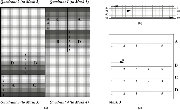
Figure 1: Geometrical layout of the VIMOS Integral Field Unit. (a) The $80\times 80$ microlenses array that form the IFU head. Each quadrant is associated with a $1600$ fibers bundle which conveys the collected light into one of the four VIMOS channels. For clarity, only details for quadrants 1 and 3 are shown. Sub-bundles group fibers associated with contiguous microlenses on each quadrant (the regions marked A, B, C, and D) and feed the four pseudo-slits on the special IFU masks put in the VIMOS focal plane. A fiber sub-bundle is in turn divided into 5 modules of 80 fibers each. The fibers in each module are aligned onto the pseudo-slits according to a complex pattern, as can be seen in (b). Panel (c) illustrates how the fiber modules are organized over the pseudo-slits in the case of the IFU Mask no. 3.

The IFU head is placed on one side of the VIMOS focal plane (see Fig. 1 in Scodeggio et al. 2005) and consists of $6400$ microlenses organized in an $80\times 80$ array. Each microlens is coupled with an optical fiber. Spatial sampling is continuous, with the dead space between fibers below $10\%$ of the fiber-to-fiber distance. The fiber bundle, which provides the optical link between the microlenses array of the IFU head and the VIMOS focal plane, is first split into 4 parts, each feeding one channel, and then distributed over “pseudo-slits” carved and properly spaced into 4 masks. Output microlenses on the pseudo-slits restore the f/15 focal ratio needed as input to the spectrograph. The IFU masks are movable devices, when the IFU observing mode is selected they are inserted in the focal plane replacing the MOS masks.

The optical configuration of the IFU guarantees that field losses do not exceed $5\%$

In Fig. 1 a schematic view of the IFU geometrical configuration is given. The microlens array of the IFU head with superimposed the division of the fiber bundle into the four VIMOS quadrants/IFU masks is described in Fig. 1 (a). Fibers going to different pseudo-slits belonging to the same IFU mask are grouped in sub-bundles, indicated with A, B, C, and D. Each sub-bundle comprises five independent modules of $20\times 4$ fibers: these are the “fundamental units” of the IFU bundle and are marked with different gray levels. The $20\times 4$ fibers in a module are re-arranged to form a linear array of $80$ fibers on a pseudo-slit (see Fig. 1 (b) for an example). Each pseudo-slit holds five fiber modules. Fig. 1 (c) shows how the modules are organized over the pseudo-slits in the case of the IFU mask corresponding to quadrant no. 3.

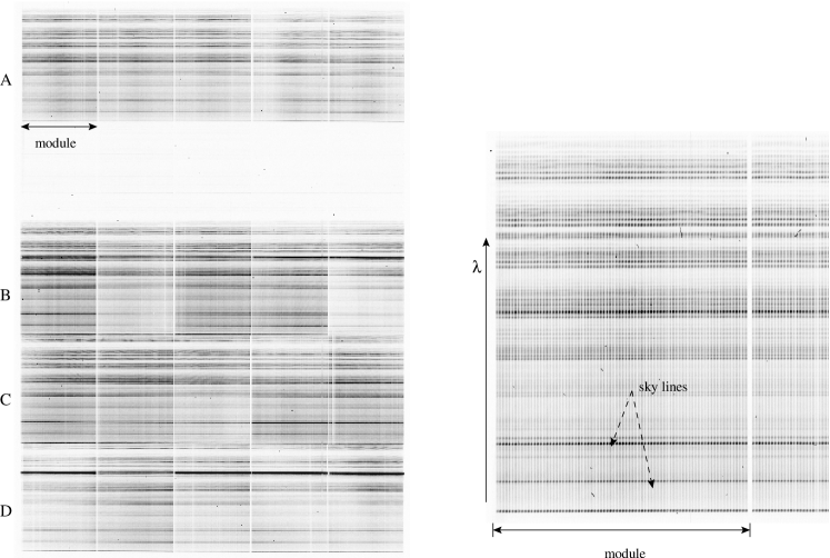
Figure 2: Left: example of an IFU exposure, only one of four quadrants is shown, the four pseudo-slits with $400$ spectra each are visible. Each spectrum spans 5 pixels in the spatial direction. One fiber module belonging to pseudo-slit A is indicated in the left panel; a zoom on the $80$ spectra coming from this module is shown in the right panel.

Contrary to what happens for MOS observations, the pseudo-slit positions on the IFU masks are fixed. This produces a fixed geometry of the spectra on the four VIMOS CCDs (see Fig. 2 for an example). The information on the correspondence between the position of a fiber in the IFU head and the position of its spectrum on the detector is one of the fundamental ingredients of the data reduction process and, together with other fiber characteristics, it is stored in the so-called “IFU table” (Sect. 3).

IFU observations can be done with any of the available VIMOS grisms (see Table 1 in Scodeggio et al. 2005). At low spectral resolution ($R\sim 200$), 4 pseudo-slits per quadrant provide $4\times 400$ horizontally stacked spectra on each of the four VIMOS CCDs. In the left panel of Fig. 2  the image of quadrant/CCD no. 3 in an IFU exposure taken with the Low Resolution Red grism is shown, the four pseudo-slits holding $400$ spectra each are clearly visible. One of the fiber modules belonging to pseudo-slit A is indicated, and a zoom on its $80$ spectra can be seen in the right panel. At high resolution ($R\approx 2500$) spectra span a much larger number of pixels in the wavelength direction over the CCDs and only the central pseudo-slit on each mask can be used. The complex rearrangement of fiber modules from the IFU head to the masks is such that the four central pseudo-slits (marked as “B” in Fig. 1) map exactly the central part of the field-of-view. This makes it possible to perform high spectral resolution observations while keeping the advantage of a contiguous field. A dedicated shutter is used to select only the central region of the IFU field-of-view.

Two different spatial resolutions, $0.67^{\prime\prime}$/fiber and $0.33^{\prime\prime}$/fiber, are possible thanks to a removable focal elongator that can be placed in front of the IFU head. The higher spatial resolution translates in a smaller field-of-view. The sky area accessible to an IFU observation is thus function of the chosen spectral and spatial samplings. Table 1 summarizes the values for the IFU field size as a function of the allowed spectral and spatial samplings.

3 The IFU Data Reduction

The IFU data reduction is part of the VIMOS Interactive Pipeline and Graphical Interface (VIPGI). For a detailed description of the VIPGI functionality as well as the handling and organization of VLT-VIMOS data we refer to Scodeggio et al. (2005).

The realization of a dedicated pipeline for the VIMOS IFU is mainly motivated by two considerations: 1) the need to be independent from already existing software environments, like IRAF or IDL ones, which was (at that time) a general ESO requirement for VLT instrument data reduction pipelines; and 2) some peculiarities of the instrument which required the development of new specific processing tools. As an example, the continuous coverage of the field-of-view does not guarantee to have dedicated fibers for pure-sky observations during each exposure. A new tool for sky subtraction (Sect. 6) has been developed, which does not require special observing techniques, like the “chopping” one, and thus does not impact on the observing overheads.

As for MOS, the starting point for the reduction of IFU data is the knowledge of an instrument model (see Sect. 4 in Scodeggio et al. (2005) for details), i.e. an optical distortion model, a curvature model and a wavelength dispersion solution. These models are periodically derived by the ESO VIMOS instrument scientists using calibration plan observations, and are stored in the image FITS headers as “first guess” polynomial coefficients. First guess parameters are used as a starting point to refine the instrument model on scientific data. With such an approach, the best possible calibration is obtained for each individual VIMOS exposure. The refinement of first guess models is a fundamental step in IFU data reduction, since the instrumental mechanical flexures are often a critical factor, see Sect. 4.1.

From the hardware point of view, each VIMOS quadrant is indeed a completely independent spectrograph, characterized by its own instrument model. For this reason IFU data processing is performed on single frames, i.e. images from each quadrant are reduced separately, up to the creation of a set of fully calibrated, 1D reduced spectra. The final steps of data reduction, like the creation of a 2D reconstructed image or the combination of exposures in a jitter sequence (Sect. 8.2), are on the contrary performed only once all images from all the quadrants have been reduced.

A high degree of automation is achieved by means of auxiliary tables needed by the data reduction procedures. In the case of VIMOS IFU, fundamental information is listed in the IFU Table. Starting from the instrument layout, this table gives the one to one correspondence between fiber position on the IFU head and spectra on the CCD, as well as other fiber parameters like the relative transmission and the coefficients describing the fiber spatial profile (see discussion in Sect. 6).

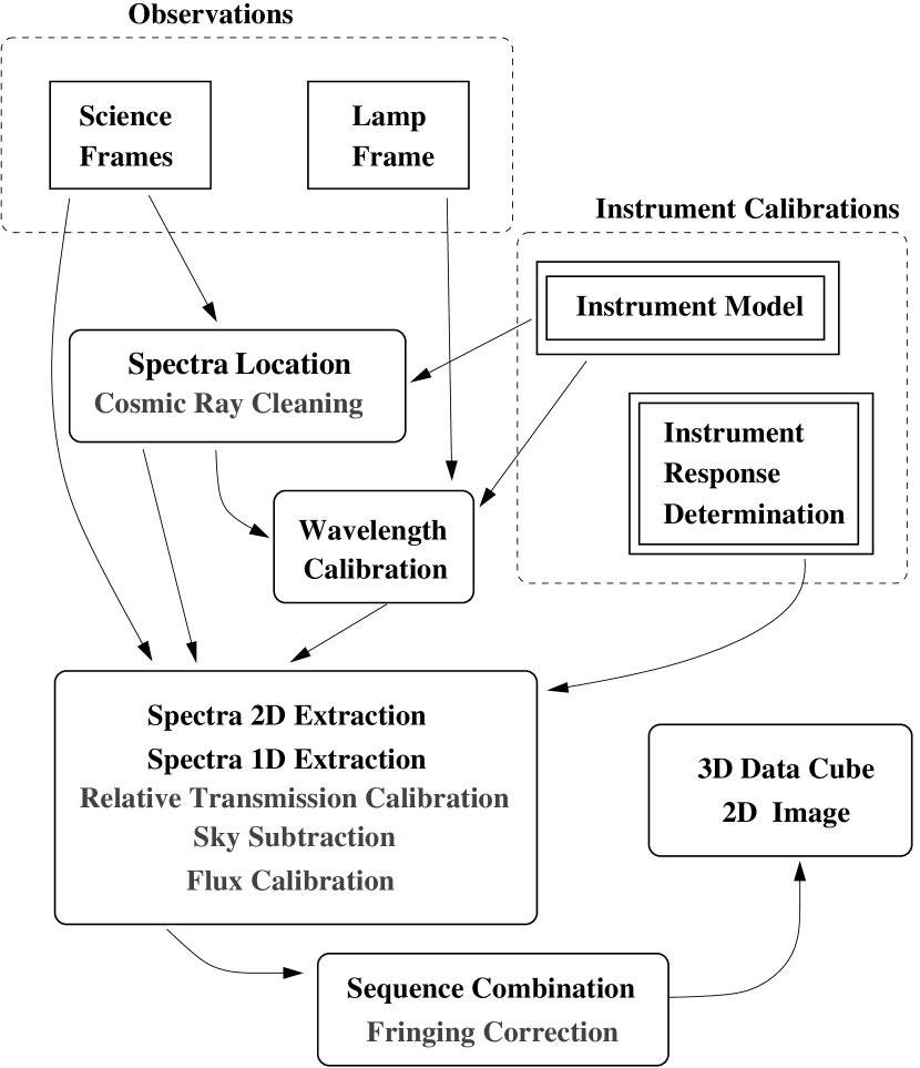
Figure 3: Block diagram showing the various steps of the reduction of VIMOS IFU data. Optional steps are marked in grey.

The first steps of IFU data reduction are: tracing of spectra on the CCD, cosmic ray cleaning and wavelength calibration – operations that lead to the extraction of 2D spectra. Wavelength calibration is performed as in the MOS case, with an accuracy of the computed dispersion solution comparable to what obtained for MOS spectra (see Scodeggio et al., 2005, for details). Extraction of 1D spectra is generally done with the usual Horne (1986) extraction method, by means of spatial profiles determined for each fiber from the data themselves. 1D extracted spectra may be calibrated to correct for differences in fiber transmission and properly combined to determine and subtract the sky spectrum. Flux calibration may be applied as a final step. If observations have been carried out using the shift-and-stare technique, 1D reduced single spectra belonging to the same sequence may be corrected for fringing and properly combined in a data cube. Finally, a 2D reconstructed image is built. A block diagram of the operations performed by the VIMOS IFU data reduction pipeline is shown in Fig. 3. In grey are marked those steps that have been left as an option. For instance, removal of cosmic ray hits as well as relative transmission correction and sky subtraction are not strictly needed in the reduction of short exposures of spectrophotometric standard stars. Moreover, sky subtraction may not satisfactorily work in the case of very crowded fields (see Sect. 6) and can be skipped. Fringing correction is not necessary when the VIMOS blue grism is used, because its wavelength range is free from such an effect.

Key steps in the processing of VIMOS IFU data are the spectra location on the CCDs, cosmic ray cleaning, cross-talk contamination and relative transmission corrections, and sky subtraction. In the following Sections we will focus our attention on these steps to clarify their impact on the data reduction and to motivate the need of dedicated reduction procedures, as well as to describe the adopted methods and to show the obtained quality.

4 Extraction of VIMOS IFU spectra

The extraction procedure consists in tracing spectra on the CCDs, applying wavelength calibration and extracting 2D and then 1D spectra. The most critical aspects of spectra extraction are the accurate location of spectra positions on the detectors and the cosmic ray cleaning; the crosstalk effect is discussed in Sect. 4.3.

4.1 Locating spectra

When dealing with VIMOS IFU data, spectra location is a much more critical step than in multi-slit mode. This is a consequence of two instrumental characteristics of the VIMOS spectrograph: mechanical flexures and spectra distribution on the detectors.

As already discussed in Section 2 of Scodeggio et al. (2005), the overall instrumental flexures induce image motion of the order of $\sim\pm 2$ pixels. In IFU mode, additional and predominant sources of mechanical instability are the deployable IFU masks, and flexures are larger than in MOS mode. Shifts of the order of $\pm 5$ pixels in the spectra positions between exposures taken at different rotation angles are typical, but values as large as $11$ pixels have been observed. Such values are comparable or larger than the spatial extent of a fiber spectrum on the VIMOS detectors (about $5$ pixels) and are strongly dependent on the instrument rotator angle during the observations.

If shifts are comparable to the spatial size of a spectrum, it may become impossible to correctly determine the correspondence between a fiber on an IFU mask and its spectrum on the detector. As can be seen in Fig. 2, the $\sim 10$ signal free pixels between modules are easily identifiable regions, and a simple user interface allows to set their (rough) position. Once an inter-module position is known, it is used as starting point from which, moving leftwards and rightwards, to measure the positions of the 80 spectra belonging to adjacent modules. The spectra positions are traced with a typical uncertainty of $0.5$ pixels. For each spectrum, a second degree polynomium is fit to these positions and its coefficients are stored in the so-called extraction table, to be used for 2D extraction. With respect to the instrument model coefficients, the extraction table gives a much more accurate description of the spectra location since it is “tuned” on the data themselves.

The spectra location method for VIMOS IFU data has been extensively tested on data taken with the different grisms and proved to be extremely robust in correctly identifying fibers and tracing spectra, irrespective of the amount of shifts induced by flexures and/or distortions.

4.2 Cosmic Ray Cleaning

Once spectra have been traced and before the 2D spectra are extracted, cleaning from cosmic ray hits is performed. This reduction step is of great importance to get a good relative transmission calibration and sky spectrum determination, since the results of these tasks can be seriously affected by the presence of uncleaned cosmic rays altering spectral intensities.

In principle, the best way to remove cosmic ray hits would be to compare different exposures of the same field. However, two reasons forced us to develop an alternative method: first, in the case of VIMOS IFU image displacements due to mechanical flexures prevent the direct comparison of pixel intensities to remove cosmic ray hits. Secondly, we were interested in having a method general enough to be applicable also in the case of single exposures of bright objects. Taking into account these considerations we developed an algorithm which works on single frames and whose principles of operations are applicable also to data taken with spectrographs other than VIMOS.

Compared to other existing tools for single-frame cosmic ray removal (e.g. the cosmicrays routine in IRAF), the method implemented in the VIMOS IFU pipeline is different because it relies on the hypothesis that - along the wavelength direction - spectra show a smooth behaviour in their intensities. In presence of emission lines or sky lines their intensity gradients will be smooth enough to be distinguishable, when compared with the abrupt changes generated by cosmic rays. This is shown in Fig. 4, where the profile of a sky line as obtained with the Low Resolution Blue grism is superimposed to the profile of a cosmic ray. Both profiles are cut along the wavelength direction.

Each IFU spectrum is traced along the CCD column by column and the intensity gradient array is computed and analyzed to search for sharp discontinuities. Intensity gradient arrays are inspected by sliding along them with a small ”window” (of the order of 20 pixels in length) inside which the local mean and rms values are computed and used to discard discrepant gradient values, likely to be due to the presence of a cosmic ray. The median and rms are re-computed on the clipped gradient window data and used to build the actual upper and lower thresholds for cosmic ray detection in the gradient window. Window size and number of sigmas to compute thresholds are user selected parameters.

Multiple pixel hits are hard to distinguish from true emission lines. In the attempt to clean as many cosmic rays as possible, without altering emission line shapes, before replacing the “suspect pixel value” we perform a further check. The mean intensity in the local window is compared with the single pixel intensities of the corresponding columns of the adjacent fibers. Because of the window dimensions (typically 20 pixels) over which the mean intensity is computed, such values should not be significantly different, except when an emission line is present. When a significant difference is found, this is interpreted as presence of an emission line, and an average of the intensities in the two comparison spectra is used as replacement value. On the contrary, if there is no difference, the intensity of pixels identified as cosmic rays is replaced with the local mean value.

Tests on spectra taken with the different VIMOS grisms showed that among all the pixels classified as cosmic ray hits on the first pass, only about $0.3\%$ actually belong to spectral lines. In all these cases, the comparison with neighbouring spectra has NOT confirmed the “cosmic ray hypothesis”, and data have not been incorrectly replaced.

It could be argued that emission lines from pointlike sources, occupying one fiber only, would be deleted by this method. In reality, given the median seeing in Paranal (0.8 $\arcsec$) and the fiber dimension on sky (0.67 $\arcsec$), such an eventuality is extremely rare.

The cosmic ray hits removal method implemented in the VIMOS IFU pipeline has been extensively tested and proved to be very efficient in cleaning both high and low spectral resolution data. On average, $\sim 90\%$ of the cosmic rays are removed: for cosmic ray hits spanning 1-2 pixels, the removal success rate is $99\%$, while more complex, extended hits are cleaned with a lower efficiency.

4.3 Crosstalk

In building the VIMOS IFU, the main drivers were the size of the field of view and a high sky sampling. This resulted in a large number of spectra (400) lying along the 2048 CCD pixels. In this situation, where each fiber projects on five pixels on the CCD, neighbouring spectra can contaminate each other, a phenomenon called “crosstalk”

The crosstalk correction must be based on the “a priori” knowledge of the fiber spatial profiles, i.e. the fiber analytic profile and its relevant parameters must be known from calibration measurements done in the laboratory on the fiber modules. For the VIMOS IFU, the fiber profiles are best described by the combination of three gaussian functions, the first one modeling the core of the fiber and the other two, symmetrical with respect to the central one, modeling the wings. The positions and widths of the gaussians can then be derived for each fiber by fitting the fiber profile on the data themselves, to get the best representation of the actual shapes and properly correct for crosstalk.

However, when applying a correction to data, it is unavoidable to introduce an error. For the correction to be effective, this error must be noticeably smaller than the effect going to be corrected. In the case of crosstalk this can only be achieved by having very good fits of the fiber profiles in the cross–dispersion direction, and we note that we have to fit a 3 parameter function on a 5 pixels profile.

To test what is the maximum discrepancy between true and measured values of the shape parameters which still allows for a good correction of crosstalk, simulations have been performed. It has been found that fiber position uncertainties of about $0.5$ pixels still guarantee that about $3/4$ of the fibers have an error in measured flux less than $5\%$, while the most critical parameter is the profile width, that must be known with noticeably higher accuracy. The quality of crosstalk correction starts to worsen quickly when the maximum error on width measurement becomes of the order of $0.2$ pixels: in such a case, the number of fibers with an accuracy in crosstalk correction worse than $5\%$ rapidly becomes greater than $50\%$ (see Fig. 5). Thus, at least for what concerns the profile width, these limiting uncertainties on the values of the profile parameters are of the same order of the accuracy we can achieve in measuring these parameters from real data.

We then estimated what is the level of crosstalk present in the real data. It turned out that on average $\sim 5\%$ of the flux of a fiber “contaminates” each neighbouring fiber, i.e. by applying the correction procedure the uncertainties we would introduce in IFU data would be of the same order of magnitude as the effect to be corrected. For this reason the crosstalk correction procedure is not currently implemented in the IFU data reduction.

5 Relative Transmission Correction

Once 1D spectra are traced and extracted from an IFU image, the next critical step is the correction for fiber relative transmission. Different fibers have different transmission efficiencies and this effect alters the intensity of spectra. This is entirely like the effect introduced by the pixel to pixel sensitivity variations in direct imaging observations, that require flatfielding of the data.

The relative transmission calibration implemented in the VIMOS IFU pipeline consists of two steps, both executable at user’s choice. First step is the correction using “standard” relative transmission coefficients that are provided by ESO as part of the instrument model calibrations and are usually determined from flat-field calibration frames. Such a standard correction cannot account for variations in relative transmission that may be due for instance to the fact that transmission degrades in time, or to variations in instrument position (e.g. rotator angle). For this reason a second step calibration is performed: a “fine” relative transmission correction is executed on the scientific data themselves, based on the sky line flux determination described below. The two steps can be executed in sequence, the second one becoming a refinement of relative transmission on the data themselves, or just one of them can be applied to the data. This choice guarantees to have the higher degree of flexibility in the data reduction procedure, thus allowing the reducer to find the best solution for the data under consideration.

The correction for fiber relative transmission is derived by imposing that the flux of sky lines must be constant in ALL fibers within one observation, and that there are no spatial variations inside the IFU field of view. The flux of a user-selected sky line is computed for each 1D spectrum, a “relative transmission” normalization factor is determined with respect to a reference fiber and it is finally applied to the 1D spectra. Sky line flux may be determined by subtracting from the line intensity the contribution of the continuum: regions on both sides of the sky line are selected and a second-order polynomial fit is done to obtain the best approximation of the continuum underlying the sky line. As will be noted in Sect. 6, the calibration of the fiber relative transmissions with the highest accuracy is of fundamental importance in order to obtain a good sky subtraction.

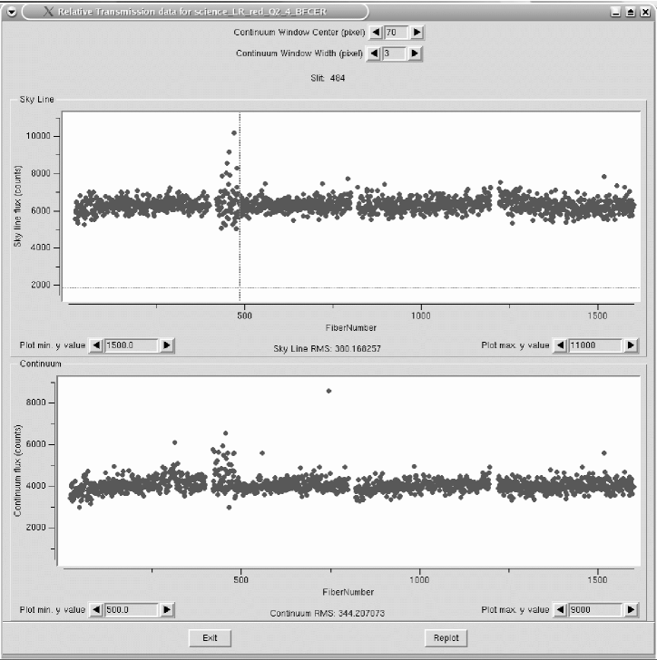
Figure 6: Graphical task for the analysis of the performance of relative transmission calibration for IFU data. The top panel shows the intensity of the $1600$ spectra at the wavelength of the skyline that has been used for the calibration (in this example the $5892$ Å  line, spectra taken with Low Resolution Red grism). The bottom panel shows again the spectral intensity, this time computed in a user–selected continuum region at $\sim 6000$ Å. The rms of the intensities is also shown for each panel.

To minimize correction uncertainties, the sky line chosen for calibrating fine relative transmission coefficients should be characterized by a fairly stable flux and be far from the fringing affected regions. In the red domain, the $5892$ Å sky line is usually a good choice, see Fig. 6 for an example. For data taken with the Low Resolution Blue grism, the $5577$ Å sky line is a very good option.

The presence of uncleaned cosmic rays altering sky line intensities would lead to an overestimate of the fiber relative transmission, preventing from obtaining a correct calibration. The occurrence of a cosmic ray hit on a given sky line is however extremely rare: for observations 45 minutes long, we statistically foresee that only $\sim 6$ spectra out of 1600 could be affected by this problem. Even if for none of them the cosmic ray removal algorithm cleaned the hits on sky lines, it would still be a negligible fraction of spectra.

An interactive plotting task may be used to verify the results of relative transmission calibration by looking for residual trends in the data at a user-selected wavelength range in the spectra. An example of the use of this task is shown in Fig. 6, where the results of applying the relative transmission calibration on an IFU exposure using the $5892$ Å  sky line are shown. In the top panel the intensity variations of the $5892$ Å  line in all the $1600$ spectra of the image are plotted, while the bottom graph shows the intensity of the continuum at $\sim 6000$ Å. Fibers 400 to 480 in Fig. 6 belong to a module characterized by a very low transmission efficiency, due to a non-optimal assembly of the optical components. The low signal from these fibers translates in a noisier determination of their relative transmission coefficients, and thus in the scatter visible in their corrected intensities.

The relative transmission calibration procedure currently implemented in the VIPGI pipeline guarantees excellent results, with differences in the corrected intensities within $5-7\%$ over all modules.

6 Sky Subtraction

Due to its design, the VIMOS IFU does not have “sky dedicated” fibers, that is fibers that are a priori known to fall on the sky. Moreover, once the light enters an optical fiber the information on its spatial distribution is lost: individual fiber spectra on the CCD do not show regions with pure sky emission and regions with object signal, as it happens in slit spectroscopy. Therefore the determination of the sky spectrum to be subtracted from the data, which is an optional operation, cannot be done in the same way as for classical spectroscopic data reduction.

IFU spectra can be either the superposition of sky background and astronomical object contribution, or pure sky background. In those cases where the field of view is relatively empty, i.e. when at least half of the fibers do not fall on an object, sky spectrum determination can be achieved by properly selecting and combining spectra which are likely to contain pure sky signal. These spectra can be selected using the histogram of the total intensities: each spectrum is integrated along the wavelength direction, and the total flux distribution is built. In a “mostly empty field” such distribution will show a peak due to pure sky spectra, plus a tail at higher intensities where object+sky spectra show up. Spectra whose integrated intensity is inside a user selected range around the peak will be pure sky spectra. A median combination of them will ensure that any residual contamination by faint objects is washed out.

The sky subtraction method implemented in the VIPGI pipeline for IFU data gives good results on deep survey observations of fields devoid of extended objects, but of course is less optimal for observations of large galaxies covering the entire field of view.

Physical characteristics of the IFU fibers/lenslets system together with the resampling executed on 2D spectra for wavelength calibration cause the fact that different fiber spectra are described by different profile shape parameters, like FWHM and skewness. Along the wavelength direction this reflects in different shapes of the spectral lines. Such effect, if not properly taken into account, affects the quality of sky subtraction: combining spectra with different line profiles would lead to an “average” sky spectrum whose lines profiles do not match with any of the original spectra, and subtracting this sky spectrum from the data would result in the presence of strong s-shape residuals.

We performed many tests on real data to determine which are the relevant profile parameters: grouping spectra according to the line FWHM value does not seem to have any influence on the goodness of sky subtraction (i.e. on the strength of the s-shape residuals). In Fig. 7 the skewness of the $5892$ Å  sky line is plotted as a function of the line width for $\sim 1600$ spectra. It can be seen from Fig. 7 that the distribution of line widths is pretty normal, and its relatively small dispersion makes it a “unimportant” parameter in the line profile description. Nevertheless, Fig. 7 shows instead a very clear bimodality in the distribution of line skewness. Such bimodality is surely an artifact deriving from the undersampling of the line profile: with a typical FWHM of $\sim 3-4$ pixels, we can only see whether skewness is positive or negative. Anyway, our tests have shown that grouping fibers according to the sign of their skewness does indeed influence the strength of residuals. A further classification according to other line shape parameters would lead to too many fiber groups, each with too few spectra to allow for a robust sky determination. Last, but not least, line shape changes across the focal plane, due to the dependence of the instrument focus and optical aberrations on the distance from the instrument (in the VIMOS case, quadrant) optical axis. For this reason, we analyze separately spectra belonging to different pseudo-slits. Thus sky subtraction consists in: grouping spectra according to the skewness of a user-selected skyline; for spectra belonging to each skewness group the distribution of total intensities is built; finally an “average” sky spectrum is computed and subtracted from all the spectra belonging to that group.

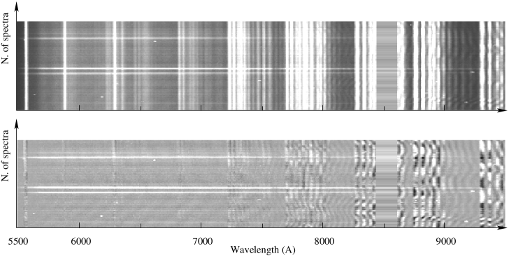
Figure 8: Example of the results obtained by the sky subtraction procedure. Top: 1D relative transmission corrected spectra in an exposure taken with the Low Resolution Red grism. Bottom: same spectra after sky subtraction. The $5892$ Å  sky line has been used to group spectra before “average” sky spectrum computation. In the $\sim 8500$ Å  region the zero order due to a nearby pseudo-slit has been clipped, originating a “flat” intensity distribution.

Given the adopted method for sky subtraction, an overall good relative transmission calibration is essential to get a correct intensity distribution and thus a proper selection of pure sky spectra. On the other hand, due to the median combination, if just some spectrum has not been perfectly corrected for fiber relative transmission, it will not affect the sky subtraction step. This sky subtraction procedure guarantees good results, with the mean level over the continuum well centered around 0 in spectra where no object signal is present, and an rms of the order of a few percent. An example of sky subtracted spectra can be seen in Fig. 8.

7 Flux calibration

The last step of data reduction on single observations is flux calibration, done in a standard way by multiplying 1D spectra by the sensitivity function derived from standard star observations. All the spectra containing flux from the standard star are summed together, and the instrument sensitivity function computed by comparison with the real standard star spectrum from the literature.

On the basis of a few objects with known magnitudes that have been observed with the VIMOS IFU, we have estimated that the overall absolute flux accuracy that can be reached with a good quality spectro-photometric calibration is of the order of $15\%$, given the unavoidable sources of uncertainty, such as cross talk contribution (of the order of 5%), relative transmission correction (between 5% and 10%) and sky subtraction (few percents).

8 Final steps: jitter sequences data reduction

The final result of the single frame reduction procedure is a FITS image, containing intermediate products of the reduction (e.g. spectra not corrected for fiber transmission, or not sky subtracted) under the form of image extensions, plus some tables used and/or created during the execution of the different tasks.

In many cases, observations had been carried out using a jittering technique (the telescope is slightly offsetted from one exposure to the next). In these cases, the spectra from the single exposures must be stacked together according to their offsets, and in this process also correction for fringing can be applied.

8.1 Correcting for fringing

Due to the characteristics of the VIMOS CCDs, when observing in the red wavelength domain, one has to deal with the fringing phenomenon, whose effects show up at wavelengths larger than $\sim 8200$ Å  in VIMOS spectra.

The decision to carry out the fringing correction at the stacking of the single exposures stage is dictated by the consideration that during a typical jitter sequence (a few hours exposure time) the fringing pattern remains relatively constant. On the contrary, the overall background intensity and the relative strength of the individual sky emission lines can vary significantly over the same time scales. Likewise, the physical location of the spectra on the CCD changes because of flexures (see Sect. 4.1 for an evaluation of flexures-induced image motions). Our approach has been to correct first for the most rapidly changing effects (first spectra location, secondly sky background) and only in the end to try to correct for fringing, which is then computed and applied on 1D extracted spectra that have already been corrected for cosmic ray hits, for relative fiber transmission, etc.

The fringing correction can only be applied on jittered observations and is performed separately for the sets of images coming from different quadrants.

First, all the spectra obtained in the jitter sequence for a given fiber are combined without taking into account telescope offsets: any object signal is thus averaged out in the combination and what remains is a good representation of the fringing pattern, which is then subtracted from each single spectrum.

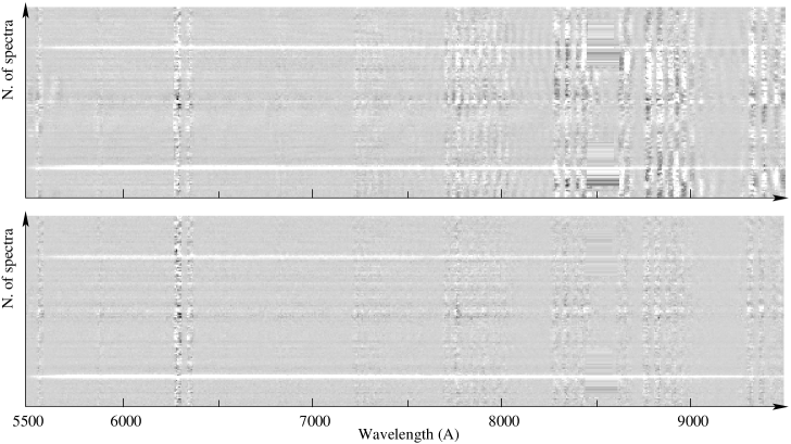
Figure 9: Efficiency of fringing correction: example of jitter–combined fully reduced sequence of 9 exposures, 26 minutes each, taken with the Low Resolution Red grism (wavelength range $5500-9500$ Å) on the Chandra Deep Field South. Each row is a different spectrum. Upper and lower panels are respectively without and with fringing correction applied to the data. As it can be seen in the lower panel, at wavelengths larger than $\sim 8200$ Å  very low fringing residuals are left after correction.

The quality of fringing correction is very good: Fig. 9 shows the result of the reduction of a sequence of 9 jittered exposures on the Chandra Deep Field South. Observations have been done using the Low Resolution Red grism (wavelength range $5500-9500$ Å, dispersion $7.14$ Å/pixel), with single frame exposure times of $26$ minutes. In Fig. 9, top, the exposures have been combined without applying any correction for fringing, while the bottom frame shows the result after having corrected for fringing as explained above. It can be seen that fringing correction is efficient in removing almost completely the residuals in the $\lambda>8200$ Å  region of the spectra.

8.2 Stacking jittered sequences of exposures

Stacking is done using all the available images from all the VIMOS quadrants at a time. In fact, due to the contiguous field of view of the VIMOS IFU and given how fibers are rearranged on the four VIMOS quadrants, an object spectrum can “move” from one quadrant to the other going from one jittered exposure to the next.

Image stacking makes use of datacubes, i.e. 3D images where the (x,y) axes sample the spatial coordinates and the z axis samples the wavelength. One datacube is created starting from the four images of each IFU exposure. Jitter offsets are computed by using the header information on telescope pointing coordinates or by means of a user-given offset list, and are used to build a final 3D image starting from single datacubes. Variations of the relative transmission from quadrant to quadrant, and inside the same quadrant from one exposure to the next one in the sequence, are taken into account by properly rescaling image intensities.

The output of the reduction procedure is a FITS image containing all the stacked 1D spectra in the final datacube: each spectrum is written in a row of the output image (see Fig. 9), and a correspondence table between the position of the spectrum in the final 3D cube appended to it.

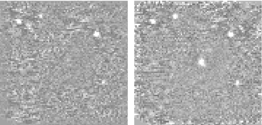
Figure 10: 2D reconstructed image of the cluster MRC1022-299 obtained by integrating over the $5800\div 8000$ Å  wavelength range (left) and over $100$ Å  centered on the radiogalaxy [OII]3727 emission line (right) redshifted at $\simeq 7100$ Å  (redshift z=0.9085). The radiogalaxy OII emission is clearly extended and asymmetric, and a velocity field can be retrieved from the 3D cube. On these images East is up and North is right. About $3\%$ of the pixels correspond to black/dead fiber spectra and have been cleaned with the IRAF task fixpix.

Finally, a 2D reconstructed image can be built for scientific analysis. In Fig. 10 we show an example of 2D reconstructed image from VIMOS IFU observations of the candidate cluster MRC1022-299 associated with a high redshift radiogalaxy (McCarthy et al., 1996; Chapman et al., 2000). A sequence of $5$ jittered exposures of $26$ minutes each taken with the Low Resolution Red grism has been combined and integrated over the wavelength range $5800-8000$ Å  (left) and over a narrow band $100$ Å  wide centered at $7100$ Å  (right), where an emission line identified with OII is observed in the radiogalaxy spectrum. The radiogalaxy, invisible in the broad-band image, shows up at the center of the field in the narrow-band image. From the OII line we got a redshift of $0.9085$ for the radiogalaxy, consistent with the value quoted by McCarthy et al. (1996).

2D reconstructed images can be built from any kind of 1D extracted spectra, e.g. transmission corrected or sky subtracted ones, by using the sky-to-CCD fiber correspondence given in the standard IFU table or, in the case of a jitter sequence reduction, in the associated correspondence table. These images are particularly useful when dealing with crowded fields data, when the automatic sky subtraction recipe cannot guarantee good results. In such cases the reduction to 1D spectra can be done without sky subtraction. A preliminary 2D image can be reconstructed and used to interactively identify fibers/spectra in object-free regions, to be later combined to obtain an accurate estimate of the sky background signal.

9 Summary

The VIMOS Integral Field Spectrograph has required a new approach to process the large amount of data produced by $6400$ micro-lenses and fibers.

The instrumental IFU setup and the packing of spectra on the $4$ VIMOS detectors has motivated the development of dedicated recipes, with the possibility to carefully check the quality of results by means of interactive tasks.

With the large amount of spectra acquired by the VIMOS IFU, it has been mandatory to implement the IFU data processing in a pipeline scheme as much automated as possible. The VIMOS IFU data processing is implemented under the VIPGI environment (Scodeggio et al., 2005) and is available to the scientific community to process VIMOS IFU data since November 2003.

We have estimated that the overall absolute flux accuracy that can be reached with our pipeline is of the order of $15\%$, the main sources of uncertainty being the cross talk contribution (significant, of the order of 5%), the relative transmission correction (between 5% and 10%) and sky subtraction (few percents).

Table 1: Characteristics of the VIMOS Integral Field Unit.

Spectral resolution	Field of View	Spatial resolution	Spatial elements	Spectral elements
		(arcsec/fiber)		(pixel)
Low (R $\sim$ 200)	$54^{\prime\prime}\times 54^{\prime\prime}$	$0.67$	6400	600
	$27^{\prime\prime}\times 27^{\prime\prime}$	$0.33$
High (R $\sim$ 2500)	$27^{\prime\prime}\times 27^{\prime\prime}$	$0.67$	1600	4096
	$13^{\prime\prime}\times 13^{\prime\prime}$	$0.33$

Figure 4: Sky line profile along the dispersion direction (continuum line), superimposed to the profile of a cosmic ray (dot-dashed line).

Figure 5: Performance of the crosstalk correction as a function of the accuracy in the measure of the fiber profile width. Solid line: number of fibers with error on the recovered flux less than $5\%$. Dashed line: error between $5\%$ and $10\%$. Dotted line: error between $10\%$ and $20\%$. Dot-dashed: error greater than $20\%$.

Figure 7: Distribution of the $5892$ Å  sky line skewness as a function of sky line width, measured for $\sim 1600$ 1D spectra.

References

- Allington-Smith & Content (1998) Allington-Smith, J. & Content, R. 1998, PASP, 110, 1216
- Allington-Smith et al. (2002) Allington-Smith, J. et al. 2002, Experimental Astronomy, 13, 1
- Bacon et al. (1995) Bacon, R. et al. 1995, A&AS, 113, 347
- Bacon et al. (2001) Bacon, R. et al. 2001, MNRAS, 326, 23
- Bonneville et al. (2003) Bonneville, C. et al. 2003, Proc. SPIE, 4841, 1771
- Chapman et al. (2000) Chapman, S. C., McCarthy, P. J., Persson, S. E. 2000, AJ, 120, 1612
- Content et al. (2000) Content, R. M. et al. 2000, Proc.SPIE, 4013, 851
- Emsellem et al. (2004) Emsellem, E. et al. 2004, MNRAS, 352, 721
- Horne (1986) Horne, K. 1986, PASP, 98, 609
- Le Fèvre et al. (2002) Le Fèvre, O. et al. 2002, The Messenger, 109, 21
- McCarthy et al. (1996) McCarthy, P. J., Kapahi, V. K., van Breugel, W. Persson, S. E., Athreya, R., Subrahmanya, C. R. 1996, ApJS, 107, 19
- Prieto et al. (2000) Prieto, E., Le Fèvre, O., Saisse, M., Voet, C., Bonneville, C., 2000, Proc, SPIE, 4008, 510
- Scodeggio et al. (2005) Scodeggio, M. et al. 2005, PASP, submitted
- Walsh & Roth (2002) Walsh, J. R. & Roth, M. M. 2002, The Messenger, 109, 54