Space and Ground Based Pulsation Data of $\eta$ Bootis Explained with Stellar Models Including Turbulence

Abstract

The space telescope MOST is now providing us with extremely accurate low frequency $p$-mode oscillation data for the star $\eta$ Boo. We demonstrate in this paper that these data, when combined with ground based measurements of the high frequency $p$-mode spectrum, can be reproduced with stellar models that include the effects of turbulence in their outer layers. Without turbulence, the $l=0$ modes of our models deviate from either the ground based or the space data by about $1.5$–$4\,\mu$Hz. This discrepancy can be completely removed by including turbulence in the models and we can exactly match $12$ out of $13$ MOST frequencies that we identified as $l=0$ modes in addition to $13$ out of $21$ ground based frequencies within their observational $2\sigma$ tolerances. The better agreement between model frequencies and observed ones depends for the most part on the turbulent kinetic energy which was taken from a 3D convection simulation for the Sun.

1 Introduction

Until now, high precision stellar modeling of the outer stellar layers was needed solely for helioseismic studies. In order to reproduce the observed solar $p$-mode oscillation frequencies, Li et al. (2002) demonstrated that the proper inclusion of turbulence improves the observed solar high frequency $p$-modes from a maximum deviation of $15\,\mu$Hz at $4000\,\mu$Hz for a model without turbulence to $5\,\mu$Hz for a model with turbulence.

The inclusion of turbulence is a twofold problem. It consists of realistically modeling turbulent convection in the outer layers and then including simulation data in stellar models. Semianalytical models for turbulent convection have been proposed by Canuto (1990, 1996). His main idea is to include a full turbulence spectrum. Canuto’s model has been included in stellar codes by Canuto & Mazzitelli (1991) and Canuto, Goldman, & Mazzitelli (1996). The free parameters in the semi-analytical model were derived from laboratory experiments of incompressible convection and extrapolated to stellar conditions. Using this approach, the superadiabatic peak is much higher than that of the standard solar model (SSM), while the derived $p$-modes are closer to the observed values than those from SSMs (Paterno et al. 1993).

In another approach, three-dimensional (3D) large eddy simulations of deep compressible convection have been first performed by Chan & Sofia (1989). While it is not possible to resolve the full turbulence spectrum in 3D simulations, the advantage of these simulations is that they are essentially parameter-free, provided that the employed subgrid model does not significantly modify the properties of the large scale dynamics. In the early studies, no account was taken of the radiative transfer in the 3D simulation, and therefore the stellar models that included a parametrized convective flux from the simulations showed a larger discrepancy with observed solar $p$-mode frequencies (Lydon, Fox, & Sofia 1992; Lydon 1993).

Part of these limitations were overcome by Kim et al. (1995, 1996) who employed the diffusion approximation for the radiation field but consequently could not include the optically thin part of the SAL. Later, Kim & Chan (1997, 1998) employed the Eddington approximation for the radiation field, included a realistic equation of state and radiative opacities. Their simulation spanned 5.5 pressure scale heights and included all of the SAL. Demarque, Guenther, & Kim (1999) mimicked the effects of the simulations in calibrated solar models by increasing the opacity coefficient $\kappa$ which decreased the discrepancy between observed and model $p$-mode frequencies.

Using different numerical methods to solve the convective and radiative equations, Stein & Nordlund (1998) also performed full 3D simulations, incorporating LTE radiative transfer and a realistic equation of state. The simulation included the entire SAL and spanned a total of 11 pressure scale heights. Rosenthal et al. (1999) used averages of Stein & Nordlund (1998)’s hydrodynamical simulations to match the simulation to an envelope that was constructed with a standard mixing length envelope code. These patched models showed a better agreement with the observed $p$-mode frequencies than earlier models.

In this paper we make use of the recently performed 3D simulations of fully compressible hydrodynamics by Robinson et al. (2003, 2004). These efforts build on the earlier work by Kim & Chan (1998). While resolving the SAL and covering $7.4$ pressure scale heights in the vertical domain, they yielded results in agreement with Stein & Nordlund (1998). Robinson et al.’s studies showed that artifacts of the boundary conditions had affected the Kim & Chan (1998) 3D simulations and they ascertained the resolution and domain sizes needed to yield physically realistic results. Using averages for the turbulent pressure and turbulent kinetic energy taken from these simulations Li et al. (2002) included these effects on the stellar structure of the one dimensional models within the mixing length theory (MLT) framework. So far, the best match to observed solar $p$-mode frequencies has been achieved with these methods.

The space mission MOST (Walker et al. 2003) is now providing us with new low frequency $p$-modes for $\eta$ Boo (Guenther et al. 2005). With the ground based measurements of the high frequency part from Kjeldsen et al. (2003), which are sensitive to the outer stellar layers of the star, we demonstrate that the combined data set can be matched within the errors when we include turbulence in the outer layers of this star. The ground based data by Carrier, Eggenberger, & Bouchy (2005) are also discussed.

2 Stellar Models

2.1 Turbulence

For the Sun, Li et al. (2002) have devised a method to include the effects of turbulence obtained from 3D hydrodynamic simulations (Robinson et al. 2003) by including both the turbulent pressure and the turbulent kinetic energy into the 1D stellar model within the framework of standard MLT. This method produces $p$-mode frequencies that match the measured solar spectrum better than an SSM without turbulence.

We slightly modify the techniques of Li et al. to enable us to apply the 3D turbulence data for the Sun to our model of $\eta$ Boo. Until we have completed a full 3D simulation for the outer layers of $\eta$ Boo, we make use of the solar data and appropriately shift the data to apply it at the correct depth in $\eta$ Boo. This shifting is motivated by an expected characteristic found in all our 3D simulations: namely that the SAL peak closely coincides with the turbulent pressure peak.

This is verified for 3D simulations of four different evolutionary stages of the Sun (ZAMS, current Sun, subgiant and giant). In each case the peak of the turbulent pressure closely coincides with the peak of the SAL. Figure 1 illustrates this property for the Sun.

Figure 1: Averaged quantities taken from a 3D turbulent convection simulation for the Sun. The peak of the SAL coincides with the peak of turbulent pressure. The inset magnifies the peak locations to show their relative positions.

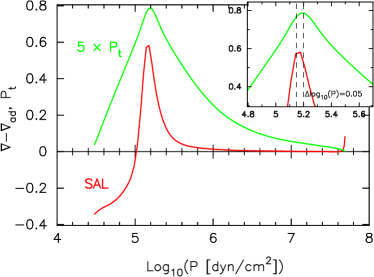
The offset between the peaks measured in pressure difference is always smaller than $\Delta\!\log_{10}(P\,[\mathrm{dyn/cm^{2}}])=0.1$. Therefore, in order to apply the solar turbulence data to $\eta$ Boo we match the turbulent pressure peak from the 3D simulation data with the SAL of the one dimensional model with a small offset of $\Delta\!\log_{10}(P\,[\mathrm{dyn/cm^{2}}])=0.0758$, a mean value derived from the four solar models. This ensures that the solar turbulence data is applied at the correct depth of the $\eta$ Boo model.

$\eta$ Boo exhibits a slightly higher effective temperature of $T_{\mathrm{eff}}=6028\,$K which amounts to a 18% higher flux compared to the Sun. The surface gravity of $\eta$ Boo is a factor of four lower. Both differences can change the relative strength of the turbulent pressure and turbulent kinetic energy in the 3D simulation but we do not have enough simulations available yet in order to extract sensible scaling relations. Therefore, no further scaling has been performed.

The refined treatment of the outer stellar layers has been implemented in the Yale Stellar Evolution Code (YREC). The numerical methods and main physics included are described by Pinsonneault (1988) and Guenther et al. (1992). The most recent improvements other than the inclusion of turbulence in the outer layers include new updates to the equation of state (OPAL 2001 EOS, Rogers 2001).

The high spatial resolution needed for the solar models is also required for the $\eta$ Boo models. A model typically consists of about $4500$ grid points which are distributed in order to give smooth runs of all variables. In contrast to the solar models we find that a more stringent time-stepping is needed for $\eta$ Boo in order to yield resolution independent $p$-mode frequencies. This is most likely due to $\eta$ Boo’s more advanced evolutionary stage. This demands us to advance the model through at least $2500$ time steps.

2.2 Starting Model

Our model construction starts from a model for $\eta$ Boo that has been selected with the quantified dense grid method (QDG) developed by Guenther & Brown (2004). The search performed for $\eta$ Boo is described in detail by Guenther et al. (2005). Their best fit model is selected from an extended search with different input parameters for hydrogen $X=(0.69,0.71)$, metallicity $Z=(0.02,0.03,0.04)$ and stellar masses between $1.4\,{M}_{\sun}$ and $1.9\,{M}_{\sun}$ with a fine grid resolution of $0.005\,{M}_{\sun}$. Along each evolution track of the models, $p$-mode frequency spectra for the $l=0,1,2,3$ modes have been calculated from radial order $n=1$ to the acoustic cutoff frequency.

A total of $3\times 10^{7}$ model frequency spectra have been compared with eight selected MOST frequency measurements that were judged to be the most likely members of the $l=0$ $p$-mode sequence. The agreement between model spectra and observation is ascertained with the $\chi^{2}$ formulation (Guenther & Brown 2004). The best model consists of a mass of $1.71\pm 0.05\,{M}_{\sun}$, $(X,Z)=(0.71,0.04)$, a mixing length of $1.8$ and no element diffusion at an evolution age of $2.40\pm 0.03\,$Gyrs. This best model with a $\chi^{2}<1.4$ was constrained only by the 8 MOST $p$-modes. No other constraints, such as composition, surface temperature, or luminosity were used. Regardless, their model which best fits the oscillation data also lies within $1\sigma$ of the observationally derived effective temperature, luminosity, and metal abundance.

A new interferometric measurement of $\eta$ Boo’s radius is now available (Thévenin et al. 2005), yielding a radius of $R/{{R}_{\sun}}=2.68\pm 0.05$. The best model selected with the QDG search technique is fully consistent with this value, since it possesses a radius of $R/{R}_{\sun}=2.6842$. Guenther et al. (2005) show that there is no other model within the searched parameter-space that fits both the MOST data and, in addition, the effective temperature and luminosity as derived observationally by Di Mauro et al. (2003). Thus, the new interferometric radius measurement does not give any additional constraint to our modeling, nevertheless it is an essential requirement that our models are consistent with this observationally determined radius.

The pulsation spectra computed for this paper are calculated from a model with exactly the same input parameters but using a slightly different version of YREC that incorporates the newer OPAL 2001 EOS. For an evolutionary age of $2.409\,$Gyrs we achieve a favorable fit of $\chi^{2}<1.0$. This model is shown in an echelle diagram in Figure 2 (green triangles). All $\chi^{2}$-numbers are calculated with an adopted model uncertainty of $0.05\,\mu$Hz, and with the exact $1\sigma$ uncertainty as quoted by the authors for their individual measurements.

Figure 2: Echelle diagram showing the non-adiabatic $p$-mode frequencies derived from a best-fit theoretical model without turbulence (triangles) in comparison to a model with turbulence (squares) on top of the ground and space based observational measurements. The eight selected MOST measurements used in the QDG search are marked with filled circles. The quoted error bars correspond to a $2\,\sigma$ deviation.

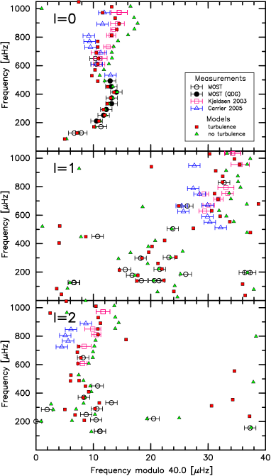
It is important to note that none of the models without turbulence – searched for giving a good $\chi^{2}$-fit for eight selected MOST low $p$-mode frequencies – match the $l=0$ ground based frequency measurements satisfactorily. The model frequencies appear to be at slightly higher folded frequencies with a difference that increases from $1.5\,\mu$Hz at $600\,\mu$Hz to $4\,\mu$Hz at $900\,\mu$Hz (Figure 2). These differences between model and observations are marginally within observational uncertainty up to $700\,\mu$Hz, but above $700\,\mu$Hz they are significant.

2.3 Model Calibration

Next we construct a neighboring model to our previously defined best fit model that yields the same good agreement to the observed MOST $p$-mode frequencies and in addition includes the effects of turbulence in the outer layers. There is a fundamental difference in calibrating models to $\eta$ Boo compared to calibrating models to the Sun. For the latter we know the age to high precision. Therefore, a solar model is calibrated by evolving the model to the exact same age and changing two unknown stellar parameters, i.e., mixing length and hydrogen mass fraction. To first order, the luminosity depends on the hydrogen mass fraction and the effective temperature is most sensitive to the mixing length parameter. By attempting to follow a similar procedure with $\eta$ Boo we are faced with the difficulty that neither the age nor the mass of this star are known. In order to fit a specific locus in the HRD we can, e.g., hold the mixing length constant and only vary the hydrogen content and the age. However, this choice is arbitrary and we could with equal justification have held either the hydrogen content or the age constant, while varying the remaining other two.

To find a proper calibration method we look at the effect on the $p$-mode frequencies of changing one of the three free parameters (mixing length, hydrogen content or age) while keeping the other two fixed. Changing the age simultaneously alters all frequencies, thus altering the age would destroy our good match with the MOST data. Turning this finding around, we can view the QDG search for a match of the lower frequency $p$-modes as a method for finding the age and locus in the HRD of $\eta$ Boo. This finding is supported by the more rigorous analysis made in Guenther et al. (2005) where it is shown that the low frequency $p$-modes anchor the interior structure, hence mass and age, effectively.

With the age and mass being fixed by the low frequency $p$-modes, we conclude that the calibration of a model with turbulence has to be performed the same way as for the Sun by changing the mixing length parameter and the hydrogen mass fraction. However, the age parameter could be used to fine-tune and improve the $\chi^{2}$-fit of the combined low and high- frequency data sets, a possibility not taken advantage of here.

3 Results

We now put together the different elements discussed in the previous sections in order to derive the pulsation spectrum of a model for $\eta$ Boo that includes turbulence. The mass, metallicity, age, luminosity and effective temperature of $\eta$ Boo is derived with the QDG search technique outlined in Section 2.2 yielding a model in the subgiant evolutionary phase at age $2.409\,$Gyrs, mass of $1.710\,{M}_{\sun}$, metallicity of $Z=0.04$ and mixing length of $1.8$ that fits eight selected $p$-mode observations of MOST with $\chi^{2}<1.0$. The non-adiabatic $p$-mode frequencies for this model are calculated with Guenther’s pulsation code JIG (Guenther 1994).

Six linear non-adiabatic equations are solved which take only into account radiative losses and gains. The convective flux is “frozen” out of the pulsation equations (see Pesnell 1990, for a description on the various ways in which this can be done) thus the coupling of convection and the oscillations is not accounted for. The calculated frequencies are shown in Figure 2. Only one of the eight frequencies in the high frequency regime matches the ground based data points reported by Kjeldsen et al. (2003), on average the model yields folded frequencies about $3\,\mu$Hz larger.

Next we include the effects of turbulence in our model according to Section 2.1. The free parameters mixing length and hydrogen abundance are adjusted slightly to ensure that the luminosity and effective temperature of the model with turbulence matched the luminosity and effective temperature of the model without turbulence. The calibration procedure is stopped after luminosity and effective temperature match with a relative difference better than $5\times 10^{-5}$.

3.1 Radial modes

Finally, the non-adiabatic $l=0,1,2\,$ $p$-mode frequency spectrum is calculated with JIG and we plot the results in an echelle diagram (Figure 2). We can see in this figure that the model with turbulence still matches the $l=0$ low frequency MOST data points as required by our calibration technique while in addition it reproduces six out of the eight ground based $l=0$ frequency data points by Kjeldsen, five within their $1\sigma$ uncertainty and one within $2\sigma$. Also note that one frequency not matching the data is still a match within $3\sigma$ and that we are using the errors as quoted by Kjeldsen et al. (2003).

The region of $600-650\,\mu$Hz where the models coincide with the two MOST modes that have been independently confirmed by the ground based measured modes of both Kjeldsen et al. (2003) and Carrier et al. (2005) add credibility to our modeling. As already noted in Guenther et al. (2005), MOST had measured two modes below $200\,\mu$Hz that also fit into the $l=0$ sequence of our models.

To provide a more quantitative measure we calculate the $\chi^{2}$ numbers for the combined data sets (MOST plus Kjeldsen et al.) of all $l=0$ modes in the range $200-900\,\mu$Hz. For the model without turbulence we get $\chi^{2}=18$ compared to $\chi^{2}=2.5$ for the model that includes turbulence.

In Guenther et al. (2005) the best fit to the combined MOST and Kjeldsen et al. modes, again only constrained by the oscillation frequencies, yielded a $\chi^{2}=2.3$. But, importantly, the model corresponding to this fit to the oscillation data, did not fit $\eta$ Boo’s location in the HRD. By including turbulence in our model, we fit the MOST oscillation data, the Kjeldsen et al. oscillation data, and the observed position in the HRD (Di Mauro et al. 2003; Thévenin et al. 2005) simultaneously.

Our model with turbulence fits the Kjeldsen data much better than the data from Carrier. The combined set of MOST plus Carrier data gives a $\chi^{2}=18$. Since the Carrier data appears consistently at lower folded frequencies, the standard model without turbulence is very far off with a $\chi^{2}=131$. Hence the model with turbulence is still much closer to the Carrier data than a model without turbulence.

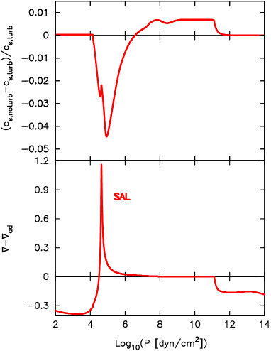
The structural difference in sound speed between the model including turbulence and without turbulence is shown in Figure 3 (top panel). As expected, the largest deviation of $\sim 4$% is seen within the peak of the SAL (bottom panel). Also, the deeper convective layers are affected by about $1$%. The structural differences vanish at pressures greater than $10^{11}\,$dyn/cm², where the layers are fully radiative.

Figure 3: Relative difference in sound speed of the outer layers of $\eta$ Boo between a model including and lacking the effects of turbulence (top panel). The SAL of the model including turbulence is shown for comparison (bottom panel).

3.2 Nonradial modes

Additional information is present in the $l=1,2$ modes. From our models we expect some regular spacings for the high frequency $p$-modes, but due to $\eta$ Boo’s advanced evolutionary stage no regular spacing should be seen for lower frequencies which are subject to strong mode bumping. Unfortunately, MOST did not see many high frequency modes and we must therefore mostly rely on the ground based data set.

We can see from Figure 2 that none of the five $l=2$ modes from Kjeldsen are matched within $2\sigma$ with the model lacking turbulence whereas four matches are achieved with the model that includes turbulence. The only mode that cannot be matched to the Kjeldsen data is one with frequency greater than $950\,\mu$Hz. Interestingly, we cannot reproduce any of the three measurements above this threshold (l=0,1,2) suggesting there is still room for improvement in our models. We identify one additional MOST mode at $648\,\mu$Hz that fits smoothly into the high frequency $l=2$ sequence. This mode is also better matched by the model including turbulence.

The matches of the model with turbulence to the $l=1$ ground based data are not as good as for $l=2$. The model including turbulence matches three out of eight measured frequencies in comparison to only two by the model without turbulence. This ratio is slightly enhanced when we include one additional mode found with MOST at $828\,\mu$Hz. The more successful fit of the $l=2$ modes can be explained with the finding of Guenther et al. (2005) who demonstrated that a slight perturbation in the model mass of $0.005\,{M}_{\sun}$ leads only to minimal changes in the $l=0$ modes but to extreme changes in the $l=1,2$ modes with particularly large impact on the $l=1$ modes.

Of the many modes smaller than $500\,\mu$Hz that are present in the MOST data we plot only those which lie near modes predicted by the models. Although there are many modes present in the MOST data very few modes are actually matched by the models and no statistical advantage of the models including turbulence can be inferred. Since observations show no evidence for any evenly spaced sequences in this frequency domain and models predict mode bumping to occur as a result of mixed $g$-modes for frequencies smaller than $350\,\mu$Hz and mixed $p$-modes within $350-600\,\mu$Hz we are simply not in the position yet to make use of this information in our models.

Of the nine nonradial modes measured by Carrier, none is matched by the standard model frequencies and only one is matched by a mode from the model that includes turbulence. As noted before for the radial data, the non radial $l=1,2$ appears at lower folded frequencies. Again, models with turbulence fit better to the Carrier data than models without turbulence but in either case there remains a large discrepancy between these observations and the models.

Finally, we list the frequencies from our theoretical models in Table 1 together with the observed frequencies. The observed modes are identified with radial orders that most closely match our theoretical models. Most of the measurements from the ground are identified with a radial order $n$ one higher than those in this work. The mixed mode character of all modes is indicated by the number $n_{g}$.

3.3 Origin of improved p-mode frequencies

The improvements of the fit between observed and model high frequency p-modes arise from structural changes in the superficial layers of the star, mainly in the SAL of the convection zone. However, it is important to note that the form of the structure change that reproduces the correct shift of the high frequency p-modes is not unique. For the Sun, Monteiro, Christensen-Dalsgaard, & Thompson (1996) demonstrated that models with a steeper and narrower SAL compared to standard MLT models can produce a frequency shift that brings these models in accord with the observed p-mode frequencies. In contrast to this, 3D simulations for the Sun (Nordlund & Stein 1999) produce an SAL stratification that is very close to standard MLT. The frequencies of high order p-modes are also predicted smaller when calculated from the average structure of the 3D simulations, hence, a better fit to observations is achieved. Nordlund & Stein (1999) attribute this frequency shift in their models to the turbulent pressure support and, in addition, to 3D effects arising from the net effect of the fluctuations of the opacity.

In the following, we explore how the inclusion of turbulence as performed in this paper changes the surface layer structure of $\eta$ Boo and we try to identify the characteristic features that lead to the correct p-mode frequency shifts. A similar analysis has been given by Li et al. (2002) for the Sun, here, we extend this analysis to $\eta$ Boo and add some more information about the role played by the shape of the SAL.

3.3.1 Turbulent Pressure

As described in Section 2.1, we account for the effects of turbulence on the stellar structure by including the turbulent pressure and turbulent kinetic energy taken from a 3D simulation for the Sun. Thus, we are able to explore the relative importance of both effects to the correct shifting of the high frequency p-modes. In order to do so, we calculate one model for $\eta$ Boo where we include the turbulent pressure alone and completely omit the turbulent kinetic energy. This model is calibrated to give the same luminosity and effective temperature and hence radius as our previous models. In Figure 4 we compare this model with turbulent pressure alone to the standard MLT model and the model including the effects of both turbulent pressure and turbulent kinetic energy.

Figure 4: Echelle diagram for a calibrated $\eta$ Boo model where only the effects of turbulent pressure are included (circles) in comparison to the standard MLT model (triangles) and our best model including the effects of turbulent pressure and turbulent kinetic energy (squares).

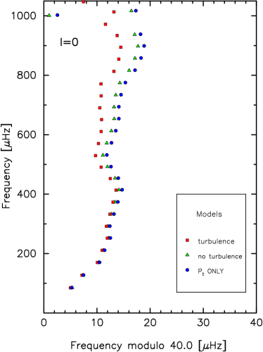
As can be seen in Figure 4, the model with turbulence alone shifts the frequencies to higher folded frequencies, hence it increases the discrepancy between the model and the observations. This finding is supported by Li et al. (2002, Fig.11), where the same effect is seen in the case of the Sun. The same behavior has been found for the Sun by Balmforth (1992, Table 1).

3.3.2 Turbulent Kinetic Energy

It is obvious from our model with turbulence alone, which fails to shift the p-mode frequencies into the right direction, that the main ingredient for a better match with observations is achieved by the effects of the turbulent kinetic energy. To show this even more clearly we have calculated one additional model in which we artificially increased the turbulent kinetic energy by a factor of two. Again, this model was properly calibrated. As can bee seen in Figure 5, increasing the turbulent kinetic energy shifts the frequencies to lower folded frequencies in the echelle diagram.

Figure 5: Echelle diagram for a calibrated $\eta$ Boo model where the turbulent kinetic energy is doubled (circles) in comparison to the standard MLT model (triangles) and our best model (squares).

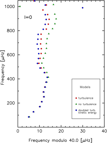
The plot also demonstrates that a quantitative match between observations and models depends crucially on the exact magnitude of the turbulent kinetic energy which we can only derive from a complete 3D simulation of the outer layers of $\eta$ Boo . Since we achieve a good fit to the $p$-mode observations by applying to our 1D model the effects of turbulent kinetic energy as derived from a 3D simulation for the Sun, it remains to be shown that a 3D simulation of the outer layers of $\eta$ Boo yields comparable values for the turbulent kinetic energy.

3.3.3 Shape of SAL

If the effects of turbulent kinetic energy can shift the model $p$-mode frequencies towards the observed frequencies, it is illuminating to find out about the structural changes that are induced by the turbulent kinetic energy onto the outer layers of $\eta$ Boo. These changes are best seen in the SAL (Figure 6).

Figure 6: The SAL for three different models: a standard MLT model (solid line), our fiducial model with turbulent pressure and turbulent kinetic energy included (dashed line) and a model with artificially increased turbulent kinetic energy (dotted line).

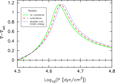
The inclusion of turbulence has the effect of shifting the peak of the SAL into deeper layers of the stellar envelope. This is the main effect responsible for the frequency shift. Also, the superadiabaticity is increased (increased peak height), but this effect is small. It is worth noticing that the shape of the SAL is preserved, with same half-maximum in all models. In order to demonstrate this, we have shifted the SAL of two models artificially to make their peak location coincide with the standard MLT model (Figure 7).

Figure 7: Same plot as Figure 6 but the models including turbulent kinetic energy have been shifted to coincide with the peak of the standard MLT model to allow for comparison of the SAL shape.

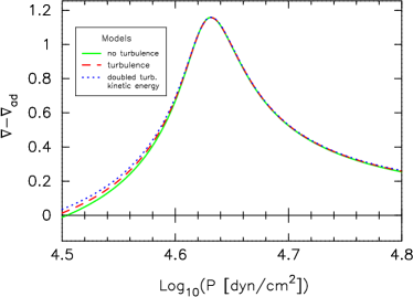
We conclude that the inclusion of turbulent kinetic energy shifts the SAL peaks into deeper layers of the stellar envelope while the shape of the SAL is preserved. The deeper SAL location changes the run of sound speed in the outer layers leading to high order $p$-mode frequency shifts towards lower folded frequencies as required by observational data for the Sun and also for $\eta$ Boo. For the latter, the exact same amount of turbulent kinetic energy as derived from a full 3D simulation for the Sun is able to bring the models in accord with the high frequency $p$-mode observations.

4 Discussion and Conclusions

This paper demonstrates that the measured $p$-mode frequencies of $\eta$ Boo from space (by MOST) and the ground (by Kjeldsen) can be jointly matched with our theoretical models by including the effects of turbulence in the outer stellar layers. We are able to report on a better match between theory and observation for a star other than the Sun when the outer stellar layers are corrected by the effects of turbulence. It is an important assumption of this paper, that the effects of turbulence on the outer layer of $\eta$ Boo can be extracted from a 3D hydrodynamical simulation of the surface layers of the Sun.

The high order $p$-mode frequency shift, that brings our model in better agreement with the observations, is shown to be a direct consequence of the inclusion of turbulent kinetic energy. Although the turbulent kinetic energy must be present in the outer convection zone, it is usually disregarded in traditional stellar modeling. The turbulent kinetic energy in this study was taken from a 3D hydrodynamical convection simulations of the Sun, therefore, only a 3D simulation for $\eta$ Boo can add the final proof that the amount of turbulent kinetic energy we use in this paper is correct.

Specifically, we show that the inclusion of turbulence into our 1D stellar evolution models, as derived from the solar 3D simulation data, can account for the difference of $1.5-4\mu\,$Hz in the echelle diagram between the ground based $l=0$ data points and the models without turbulence. The quantitative agreement for the model including turbulence is excellent for the combined data set (MOST plus Kjeldsen) of the $l=0$ $p$-mode frequencies between $200-900\,\mu$Hz with a $\chi^{2}=2.5$.

The better agreement between the observations and the models that include turbulence, is strengthened by comparing the observed ground based $l=1,2$ modes. The model with turbulence matches four out of nine $l=1$ and five out of six $l=2$ modes. If we combine all $22$ observed ground based modes with $14$ selected MOST modes, a model with turbulence reproduces $27$ modes versus $14$ modes for a model without turbulence (within $2\sigma$ error bars).

MOST sees more spectrum peaks than shown in our echelle diagrams. The models predict, that we should be seeing mixed modes. However, the stellar origin has to be established with more certainty. This will be possible with the scheduled re-observation of $\eta$ Boo by MOST in 2005. If some of the recurring peaks can be identified as nonradial modes, this will give us excellent additional information to test our models.

Because our theoretical models match the Kjeldsen data, they are not a good match to the Carrier data, since both data sets do not overlap for the majority of modes which is true for both radial and nonradial modes. Regardless of this discrepancy, frequencies from models that include turbulence come much closer to the Carrier measurements.

Certainly the most important advancement for this study is the inclusion of the turbulence data derived from a full 3D turbulence simulation for $\eta$ Boo. We are currently undertaking this task and will report on it in the future. Also, the QDG search – already being very extensive – must be expanded in the searched parameter space of hydrogen content, metallicity and convective core overshoot.

The refinements of stellar evolution theory with regard to turbulent convection in the outer layers has previously been motivated by attempts to gain a better match between theory and observation for the frequency spectrum of the Sun. This study indicates that these refinements to the theoretical models are also important for interpreting the observational data of $\eta$ Boo. We believe that the need for extremely precise theoretical models will continue to grow as more and more observational measurements become available within the young field of asteroseismology.

Table 1: Model Frequencies and Observed Frequencies

			Model Frequencies		Observations
Order	$n_{p}$	$n_{g}$	With Turbulence	Without Turbulence	MOST 2005	Kjeldsen 2003	Carrier 2005
$l=0$	$\phantom{0}1$	$\phantom{0}0$	$\phantom{0}127.17$	$\phantom{0}127.35$	$126.66$/$127.91$
	$\phantom{0}2$	$\phantom{0}0$	$\phantom{0}170.08$	$\phantom{0}170.31$	$171.32$
	$\phantom{0}3$	$\phantom{0}0$	$\phantom{0}210.96$	$\phantom{0}211.18$	$210.56$
	$\phantom{0}4$	$\phantom{0}0$	$\phantom{0}251.95$	$\phantom{0}252.19$	$251.79$
	$\phantom{0}5$	$\phantom{0}0$	$\phantom{0}291.78$	$\phantom{0}292.04$	$292.25$
	$\phantom{0}6$	$\phantom{0}0$	$\phantom{0}332.45$	$\phantom{0}332.73$	$333.17$
	$\phantom{0}7$	$\phantom{0}0$	$\phantom{0}373.02$	$\phantom{0}373.40$	$373.20$
	$\phantom{0}8$	$\phantom{0}0$	$\phantom{0}413.60$	$\phantom{0}414.14$	$414.01$
	$\phantom{0}9$	$\phantom{0}0$	$\phantom{0}452.51$	$\phantom{0}453.40$	$453.13$
	$10$	$\phantom{0}0$	$\phantom{0}490.78$	$\phantom{0}491.96$	$492.92$
	$11$	$\phantom{0}0$	$\phantom{0}529.73$	$\phantom{0}531.11$			$533.0$
	$12$	$\phantom{0}0$	$\phantom{0}570.29$	$\phantom{0}571.84$
	$13$	$\phantom{0}0$	$\phantom{0}610.78$	$\phantom{0}612.71$	$610.55$	$\phantom{0}611.0\pm 0.5$	$610.6$
	$14$	$\phantom{0}0$	$\phantom{0}650.87$	$\phantom{0}653.25$	$650.37$	$\phantom{0}651.2\pm 0.6$
	$15$	$\phantom{0}0$	$\phantom{0}690.51$	$\phantom{0}693.21$		$\phantom{0}690.8\pm 0.6$	$691.3$
	$16$	$\phantom{0}0$	$\phantom{0}730.78$	$\phantom{0}733.54$		$\phantom{0}732.6\pm 0.4$	$729.5$
	$17$	$\phantom{0}0$	$\phantom{0}770.76$	$\phantom{0}774.30$			$769.4$
	$18$	$\phantom{0}0$	$\phantom{0}813.18$	$\phantom{0}816.05$		$\phantom{0}813.1\pm 0.4$	$809.2$
	$19$	$\phantom{0}0$	$\phantom{0}854.09$	$\phantom{0}857.15$		$\phantom{0}853.6\pm 0.3$
	$20$	$\phantom{0}0$	$\phantom{0}894.48$	$\phantom{0}897.71$		$\phantom{0}894.2\pm 0.6$	$891.6$
	$21$	$\phantom{0}0$	$\phantom{0}933.80$	$\phantom{0}937.09$
	$22$	$\phantom{0}0$	$\phantom{0}971.60$	$1000.99$		$\phantom{0}974.5\pm 0.7$	$971.9$
$l=1$	$\phantom{0}1$	$20/22$	$\phantom{0}116.00$	$\phantom{0}104.19$
	$\phantom{0}1$	$18$		$\phantom{0}125.92$
	$\phantom{0}2$	$17$	$\phantom{0}137.60$
	$\phantom{0}2$	$16$	$\phantom{0}142.30$	$\phantom{0}140.52$
	$\phantom{0}2$	$12/10$	$\phantom{0}177.76$	$\phantom{0}177.22$
	$\phantom{0}3$	$12$		$\phantom{0}185.19$
	$\phantom{0}3$	$11$		$\phantom{0}196.86$
	$\phantom{0}3$	$10$	$\phantom{0}214.53$
	$\phantom{0}3$	$\phantom{0}9$	$\phantom{0}221.96$	$\phantom{0}221.40$
	$\phantom{0}4$	$\phantom{0}6/8$	$\phantom{0}261.27$	$\phantom{0}259.47$
	$\phantom{0}5$	$\phantom{0}7$	$\phantom{0}298.48$	$\phantom{0}294.38$
	$\phantom{0}5$	$\phantom{0}6$	$\phantom{0}304.40$	$\phantom{0}303.45$
	$\phantom{0}6$	$\phantom{0}4/6$	$\phantom{0}339.66$	$\phantom{0}336.48$
	$\phantom{0}6$	$\phantom{0}5$		$\phantom{0}345.58$
	$\phantom{0}7$	$\phantom{0}3$		$\phantom{0}379.58$
	$\phantom{0}8$	$\phantom{0}2$	$\phantom{0}380.22$
	$\phantom{0}8$	$\phantom{0}5$	$\phantom{0}404.03$
	$\phantom{0}8$	$\phantom{0}4/2$	$\phantom{0}422.43$	$\phantom{0}420.77$
	$\phantom{0}9$	$\phantom{0}2$	$\phantom{0}448.69$	$\phantom{0}447.84$
	$10$	$\phantom{0}2$	$\phantom{0}477.37$	$\phantom{0}476.78$
	$10$	$\phantom{0}3$		$\phantom{0}503.67$
	$11$	$\phantom{0}4$	$\phantom{0}507.43$				$512.2$
	$11$	$\phantom{0}3$	$\phantom{0}524.14$	$\phantom{0}521.11$
	$12$	$\phantom{0}1$	$\phantom{0}553.78$	$\phantom{0}554.48$			$550.3$
	$13$	$\phantom{0}1/3$	$\phantom{0}592.10$	$\phantom{0}593.18$			$589.9$
	$14$	$\phantom{0}3$	$\phantom{0}630.64$	$\phantom{0}631.91$		$\phantom{0}629.4\pm 0.3$	$625.7$
	$14$	$\phantom{0}2$	$\phantom{0}664.90$	$\phantom{0}658.58$		$\phantom{0}670.1\pm 0.5$	$665.4$/$669.9$
	$15$	$\phantom{0}2$	$\phantom{0}678.77$	$\phantom{0}676.75$
	$16$	$\phantom{0}2$	$\phantom{0}711.75$	$\phantom{0}713.97$		$\phantom{0}711.8\pm 0.4$
	$17$	$\phantom{0}2$	$\phantom{0}751.13$	$\phantom{0}753.68$		$\phantom{0}749.3$/$753.4\pm 0.5$	$748.5$
	$18$	$\phantom{0}2$		$\phantom{0}795.64$		$\phantom{0}793.1\pm 0.7$	$787.4$
	$19$	$\phantom{0}2$	$\phantom{0}832.52$	$\phantom{0}835.22$
	$20$	$\phantom{0}2$	$\phantom{0}872.54$	$\phantom{0}875.18$
	$20$	$\phantom{0}1$	$\phantom{0}911.33$	$\phantom{0}913.13$
	$21$	$\phantom{0}1$	$\phantom{0}940.11$	$\phantom{0}927.53$
	$22$	$\phantom{0}1$	$\phantom{0}955.52$	$\phantom{0}956.82$		$\phantom{0}955.6\pm 0.8$	$947.6$
	$23$	$\phantom{0}1$	$\phantom{0}994.58$	$\phantom{0}997.34$
	$24$	$\phantom{0}1$	$1030.27$	$1033.29$		$1034.3\pm 0.7$
$l=2$	$\phantom{0}1$	$30$		$\phantom{0}129.65$
	$\phantom{0}2$	$25$		$\phantom{0}157.49$
	$\phantom{0}2$	$23$		$\phantom{0}219.36$
	$\phantom{0}3$	$19$		$\phantom{0}200.90$
	$\phantom{0}3$	$18$	$\phantom{0}208.41$	$\phantom{0}206.27$
	$\phantom{0}3$	$16$		$\phantom{0}224.96$
	$\phantom{0}4$	$16$	$\phantom{0}237.23$
	$\phantom{0}4$	$15/14$	$\phantom{0}246.81$	$\phantom{0}250.28$
	$\phantom{0}5$	$13$	$\phantom{0}285.04$	$\phantom{0}283.02$
	$\phantom{0}5$	$12$	$\phantom{0}290.29$	$\phantom{0}286.99$
	$\phantom{0}5$	$11$	$\phantom{0}310.59$
	$\phantom{0}6$	$11$		$\phantom{0}322.63$
	$\phantom{0}6$	$10$	$\phantom{0}331.04$	$\phantom{0}328.29$
	$\phantom{0}6$	$\phantom{0}9$	$\phantom{0}354.29$
	$\phantom{0}7$	$\phantom{0}9$	$\phantom{0}368.25$	$\phantom{0}368.51$
	$\phantom{0}8$	$\phantom{0}8$	$\phantom{0}409.19$	$\phantom{0}409.66$
	$\phantom{0}9$	$\phantom{0}7$	$\phantom{0}448.62$	$\phantom{0}449.46$
	$\phantom{0}9$	$\phantom{0}6$		$\phantom{0}477.88$
	$10$	$\phantom{0}7$	$\phantom{0}486.02$
	$10$	$\phantom{0}6$	$\phantom{0}487.51$	$\phantom{0}488.28$
	$11$	$\phantom{0}6$	$\phantom{0}526.09$	$\phantom{0}527.45$
	$11$	$\phantom{0}5$	$\phantom{0}554.59$
	$13$	$\phantom{0}5$	$\phantom{0}607.32$	$\phantom{0}609.20$		$\phantom{0}608.1\pm 0.4$
	$14$	$\phantom{0}4$	$\phantom{0}647.83$	$\phantom{0}649.90$
	$15$	$\phantom{0}4$	$\phantom{0}687.22$	$\phantom{0}689.95$
	$16$	$\phantom{0}4$	$\phantom{0}727.43$	$\phantom{0}730.17$		$\phantom{0}728.4\pm 0.6$	$724.5$
	$17$	$\phantom{0}3$	$\phantom{0}775.69$	$\phantom{0}770.39$			$765.6$
	$18$	$\phantom{0}3$	$\phantom{0}810.81$	$\phantom{0}798.35$		$\phantom{0}810.5\pm 0.4$	$805.1$
	$19$	$\phantom{0}3$	$\phantom{0}850.78$	$\phantom{0}853.81$		$\phantom{0}849.9\pm 0.7$	$846.1$
	$20$	$\phantom{0}3$	$\phantom{0}891.24$	$\phantom{0}894.42$			$888.7$
	$21$	$\phantom{0}3$	$\phantom{0}930.84$	$\phantom{0}933.81$
	$22$	$\phantom{0}2$	$\phantom{0}962.48$	$\phantom{0}965.38$		$\phantom{0}971.7\pm 0.6$