MASS MEASUREMENTS OF AGN FROM MULTI-LORENTZIAN MODELS OF X-RAY VARIABILITY. I.
SAMPLING EFFECTS IN THEORETICAL MODELS OF THE $\sigma^{2}_{\rm rms}$-${\thinspace M_{\rm BH}}$ CORRELATION

Abstract

Recent X-ray variability studies on a large sample of Active Galactic Nuclei (AGN) suggest that the $log$ of the square of the fractional rms variability amplitude, $\sigma^{2}_{\rm rms}$, seems to correlate with the $log$ of the black-hole mass, ${\thinspace M_{\rm BH}}$, with larger black holes being less variable for a fixed time interval. The fact that the rms amplitude can be easily obtained from the observed X-ray light curves has motivated the theoretical modeling of the $\sigma^{2}_{\rm rms}$-${\thinspace M_{\rm BH}}$ correlation with the aim of constraining AGN masses based on X-ray variability. A viable approach to addressing this problem is to assume an underlying power spectral density with a suitable mass dependence, derive the functional form of the $\sigma^{2}_{\rm rms}$-${\thinspace M_{\rm BH}}$ correlation for a given sampling pattern, and investigate whether the result is consistent with the observations. Inspired by the similarities shared by the timing properties of AGN and X-ray binaries, previous studies have explored model power spectral densities characterized by broken power laws. For simplicity these studies have in general ignored the distorting effects that the particular sampling pattern used to obtain the observations imprints in the observed power spectral density. With the advent of RXTE, however, it has been shown that the band-limited noise spectra of X-ray binaries are not broken power laws but can often be described in terms of a small set of broad Lorentzians, with different amplitudes and centroid frequencies. Motivated by the latest timing results from X-ray binaries, we propose that AGN broad-band noise spectra consist of a small number of Lorentzian components. This assumption allows, for the first time, to fully account for sampling effects in theoretical models of X-ray variability in an analytic manner. We show that, neglecting sampling effects when deriving the fractional rms from the model power spectral density can lead to underestimating it by a factor of up to $80\%$ with respect to its true value for the typical sampling patterns used to monitor AGN. We discuss the implications of our results for the derivation of AGN masses using theoretical models of the $\sigma^{2}_{\rm rms}$-${\thinspace M_{\rm BH}}$ correlation.

1. Introduction

Most of the known accreting compact objects emitting in the X-ray band, both in our and other galaxies, show large variations in their fluxes (up to a factor of a few or even more in some cases) over several decades in frequency. X-ray binaries, hosting neutron stars and black holes with masses between $1\hbox{$\rm\thinspace M_{\odot}$}$ and $10\hbox{$\rm\thinspace M_{\odot}$}$, are known to be variable on time scales ranging from milliseconds up to several days (see van der Klis, 2005, for a recent review). The X-ray emission from Active Galactic Nuclei (AGN), on the other end of the mass spectrum, with masses in the range $10^{6}\hbox{$\rm\thinspace M_{\odot}$}$ to $10^{9}\hbox{$\rm\thinspace M_{\odot}$}$, fluctuates on time scales ranging from a few minutes up to a few years (e.g., Marshall, Warwick, & Pounds, 1981; Mushotzky, Done, & Pounds, 1993). The origin of this strong variability is currently not understood.

From the theoretical point of view, the main goal of variability studies is to understand the physical processes that modulate the emission of high-energy radiation and, in particular, how the fundamental properties of the central compact object (mass, spin, surface or lack thereof) determine the spectrum of observed frequencies. From the phenomenological point of view, observations provide a powerful tool for constraining mathematical models which, in turn, provide a guide in the investigation of physical models that can account for the observed variability. The studies carried out over the last decade with the Advanced Satellite for Cosmology and Astrophysics (ASCA) and the Rossi X-ray Timing Explorer (RXTE) and, more recently, with the Chandra X-ray Observatory and XMM-Newton have revolutionized the timing phenomenology of both X-ray binaries and AGN.

In the case of galactic sources, because of the typical timescales involved and thanks to the unprecedented timing capabilities of RXTE, it has become possible to derive the power spectral density (hereafter the power spectrum) of a large number of accreting binaries with exquisite detail (see e.g., van der Klis, 2005). This made possible an important step forward toward understanding the similarities and differences exhibited in the power spectra of neutron stars and black holes (Miyamoto et al., 1994; van der Klis, 1994; Sunyaev & Revnivtsev, 2000; Belloni, Psaltis, & van der Klis, 2002)

Recently, it has become evident that the most salient timing features present in many X-ray binaries can be well described by a small number of Lorentzians with different centroid frequencies, widths, and amplitudes (Nowak, 2000; Belloni, Psaltis, & van der Klis, 2002). This phenomenological framework has provided a solid ground for studying a number of tight correlations exhibited by the parameters characterizing the different Lorentzian components. Surprisingly, these correlations are not only present in any given source but are also maintained across sources (both neutron stars and black holes) over several decades in frequency space (Wijnands & van der Klis, 1999; Psaltis, Belloni, & van der Klis, 1999; Belloni, Psaltis, & van der Klis, 2002). Some of these correlations might even be present in white-dwarf systems, extending the range of their validity to lower frequencies by two orders of magnitude (Warner & Woudt, 2002; Mauche, 2002). The study, and eventual understanding, of these correlations offers one of the most promising avenues for constraining theoretical models of X-ray variability in accreting binaries.

The lower observed fluxes and longer timescales associated with AGN have not made possible a comparable progress in our understanding of their timing properties. Both of these aspects affect the characterization of the power spectrum from the data at high and low frequencies, but also, through sampling effects, within the accessible frequency range. If there is significant variability below or above the lowest and/or highest frequencies probed by the observations, then the estimation of the power spectrum from the data suffers from the effects of red noise leakage and aliasing (see, e.g., Deeming, 1975; Priestley, 1989; van der Klis, 1989; Press et al., 1992).

In the last few years, however, it has become clear that AGN power spectra do present characteristic frequencies (“breaks”) on the scale of hours to months (Edelson & Nandra, 1999; Uttley et al., 2002; Markowitz et al., 2003). These frequencies have been linked to similar characteristic frequencies detected in early observations of a number of galactic black-hole candidates (see, e.g., Belloni & Hasinger, 1990). Moreover, there is a growing body of evidence suggesting that the similarities shared by the X-ray variability of AGN and X-ray binaries extends beyond the overall shape of their power spectra. These similarities encompass a strong linear correlation between the rms variability amplitude and the X-ray flux, time scale-dependent lags between the hard and soft X-ray bands, and a similar energy-dependence of the power spectrum shape with higher energies showing flatter slopes above the frequency break (Uttley & McHardy, 2004, and references therein). The remarkable similarities shared by the global timing properties of objects with masses that differ so widely and the fact that the characteristic dynamical frequencies observed in AGN seem to correlate with mass, has encouraged the use of X-ray variability as a mean for estimating supermassive black-holes masses. Two different approaches are in use.

For the handful of AGN for which there are good available data covering a long period of time, it is possible to identify one (and in a few cases two) characteristic frequency(ies) in their power spectrum. Assuming that the same characteristic frequency can be identified in a galactic black hole of known mass (usually Cyg X-1) and that the characteristic break frequency scales inversely with mass, the mass of several AGN can be inferred (Uttley et al., 2002; Markowitz et al., 2003; McHardy et al., 2004, 2005).

As it is most often the case, however, the sparsity of the available data does not permit a reliable estimation of the power spectrum. In these cases, it is still possible to quantify the variability directly from the observed light curves by calculating the fractional rms variability amplitude (or simply fractional rms), $\sigma_{\rm rms}$, i.e., the square root of the variance of the light curve normalized by the mean flux over the period of observation after subtracting the experimental noise (see, e.g., Nandra et al., 1997). Obtaining variances from X-ray light curves is a much less intensive observational task than obtaining reliable power spectra. As a result, the fractional rms variability has been measured for a relatively large sample of AGN for a variety of sampling patterns with ASCA, RXTE, and, more recently, with Chandra and XMM-Newton.

Possible correlations between the square of the fractional rms and the X-ray luminosity have been studied in the past (Nandra et al., 1997; Turner et al., 1999; Markowitz & Edelson, 2001). More recently, the availability of mass estimates for a large number of AGN (see Woo & Urry, 2002, for a recent compilation of $\simeq 300$ masses) has allowed the study of correlations between $\sigma^{2}_{\rm rms}$ and black-hole mass, ${\thinspace M_{\rm BH}}$ (Lu & Yu, 2001; Bian & Zhao, 2003; Markowitz & Edelson, 2004; O’Neill et al., 2005). The fact that larger black holes are less variable for a given observation period suggests that the observed (anti)correlation is partially due to a corresponding difference in the size of the X-ray emitting region.

The fact that the fractional rms can be easily obtained from the observed X-ray light curves, and that the number of AGN with measured variances is rapidly increasing, has motivated the theoretical modeling of the $\sigma^{2}_{\rm rms}$-${\thinspace M_{\rm BH}}$ correlation. A fruitful approach to addressing this problem is to assume a functional form for the underlying power spectrum that depends on mass, $P(\nu;{\thinspace M_{\rm BH}})$, and calculate the square of the fractional rms that one would obtain when observing according to some sampling pattern, i.e., $\sigma^{2}_{\rm rms}(\Delta t_{\rm o},\Delta t_{\rm s},\Delta t_{\rm b},M_{\rm BH})$. Here, the set of values $\{\Delta t_{\rm o},\Delta t_{\rm s},\Delta t_{\rm b}\}$ stands for the duration of the observation, the sampling interval, and the binning interval respectively.

The connection between the rms variability and the underlying power spectrum is crucial in theoretical models of the $\sigma^{2}_{\rm rms}$-${\thinspace M_{\rm BH}}$ correlation. As a first approximation, previous works (Papadakis, 2004; Nikolajuk, Papadakis, & Czerny, 2004, but see also O’Neill et al. 2005) have assumed that the relationship between the observed fractional rms and the underlying (model) power spectrum is given by

$$\sigma^{2}_{\rm rms}(\Delta t_{\rm o},\Delta t_{\rm s},\Delta t_{\rm b},M_{\rm BH})=2\int_{1/\Delta t_{\rm o}}^{1/2\Delta t_{\rm s}}\!\!P(\nu;M_{\rm BH})~{}d\nu~{},$$ (1)

where sampling effects are considered on the right hand side only through the finite limits of integration. To our knowledge, however, a systematic study addressing how good this approximation is for the typical sampling patterns employed in AGN observations has not been carried out yet.

In this paper, motivated by current detailed timing studies of X-ray binaries, we consider model AGN band-limited noise spectra that can be described as a sum of Lorentzian components. This framework exposes (and allows to explore further) the underlying assumption often made when measuring AGN masses by comparing their power spectra with those of X-ray binaries, i.e., that the global timing properties of both systems simply “scale” with mass. An appealing feature of this framework is that it allows an analytical approach to account for the effects that the sampling pattern imprints on the observed power spectrum, facilitating the inclusion of sampling effects in theoretical models of the $\sigma^{2}_{\rm rms}$-${\thinspace M_{\rm BH}}$ correlation.

The paper is organized as follows. In §2 we discuss, from first principles, how the underlying power spectrum, whatever its functional form may be, differs from the observed power spectrum due to the finite and discrete nature of the observations. In §3 we motivate the use of Lorentzians to model the broad-band noise spectra of AGN and find an analytical expression to account for sampling effects in this type of models. In §4 we demonstrate the excellent agreement between our analytical results and Monte Carlo simulations designed to account for the distortions suffered by the underlying power spectral density due to sampling effects. Finally, in §5 we discuss the potential implications of neglecting sampling effects in theoretical models when deriving masses from the $\sigma^{2}_{\rm rms}$-${\thinspace M_{\rm BH}}$ correlation. For convenience, some of the mathematical details are presented in the appendices.

While writing this paper, we became aware of a calculation similar to the one that we present in §2 carried out by O’Neill et al. (2005). Their derivation accounts for sampling effects directly in the power spectrum as they would be present due to discrete sampling in a “continuous” monitoring campaign (i.e., $\Delta t_{\rm s}=\Delta t_{\rm b}$). The derivation that we present here is more general and shows explicitly how the different processes which one subjects the light curve to (i.e., binning, sampling, and segmentation), affect the observed power spectrum for a sampling pattern characterized by the set of values $\{\Delta t_{\rm o},\Delta t_{\rm s},\Delta t_{\rm b}\}$. In this sense, our derivation is more along the lines of van der Klis (1989), explicitly showing what happens to the real light curve in the process of obtaining the data.

2. Sampling Effects in The Power Spectrum

From the theoretical point of view, it is common to model and characterize the spectral content of a variable stochastic process by specifying the underlying (or model) power spectrum, $P(\nu)$, as a continuous function of the frequency $\nu$. This spectrum can be thought of as associated with a process, $C(t)$, that varies over time in a continuous way. In the context of X-ray variability, $C(t)$ could be given by the “underlying” (as opposed to observed) continuous and infinite X-ray light curve. In principle, complete knowledge of the observable $C(t)$ implies complete knowledge of the underlying spectrum, $P(\nu)$, and vice versa. Therefore, if we had unlimited access to the X-ray light curve, we could reconstruct the underlying power spectrum accurately for every frequency.

In practice, however, we do not have access to the continuous light curve, $C(t)$, but rather to a finite and discrete set of values $\{C_{\rm o}(t_{n})\}$ that results from observing the source for a period of time $\Delta t_{\rm o}$ every $t_{n}\equiv n\Delta t_{\rm s}$, where $\Delta t_{\rm s}$ is the inverse of the sampling rate and $n=0,...,N-1$ (without loss of generality we will assume here that $N\equiv\Delta t_{\rm o}/\Delta t_{\rm s}$ is even). In order to work with reasonably good signal-to-noise ratios, the data are usually binned for an interval of time $\Delta t_{\rm b}\leq\Delta t_{\rm s}$ (objects are said to be monitored “continuously” when $\Delta t_{\rm s}\equiv\Delta t_{\rm b}$). In what follows we will refer to the set of values $\{\Delta t_{\rm o},\Delta t_{\rm s},\Delta t_{\rm b}\}$ as the “sampling pattern”.

The finite and discrete nature of the observations not only dictates that we only have access to a finite and discrete set of values of the observed power spectrum, i.e., $\{P_{\rm o}(\nu_{k})\}$, with $\nu_{k}=k/\Delta t_{\rm o}$ and ${k=-N/2-1,...,N/2}$, but also that, through the effects of red noise leakage and aliasing (Deeming, 1975; van der Klis, 1989), these values do not coincide with the values of the underlying (model) power spectrum at those frequencies (i.e., $\{P_{\rm o}(\nu_{k})\}\neq\{P(\nu_{k})\}$). Moreover, because of the stochastic nature of the underlying process, the observed values $\{P_{\rm o}(\nu_{k})\}$ differ, in general, from observation to observation. For a stationary process, however, the average taken over different observations (with the same sampling pattern), is well defined and it can be used as a consistent estimator of the underlying power spectrum (Priestley, 1989; Press et al., 1992). The aim of this section is to find an equation that relates the continuous underlying power spectrum, $P(\nu)$, with the set of values $\{\langle P_{\rm o}(\nu_{k})\rangle\}$ obtained by averaging several observations with the same sampling pattern.

Because our goal is to find an equation that involves the model power spectrum, $P(\nu)$, we need to work with continuous functions. In order to do so, we describe the set of observed values $\{C_{\rm o}(t_{n})\}$ in terms of the continuous variable $t$, representing the time, as follows

$$C_{\rm o}(t) = C_{bin}(t;\Delta t_{\rm b})\,W_{fin}(t;\Delta t_{\rm o},\Delta t_{\rm s})~{}.$$ (2)

In this expression,

$$C_{bin}(t;\Delta t_{\rm b})=\frac{1}{\Delta t_{\rm b}}\int_{-\infty}^{\infty}C(t^{\prime})\,W(t-t^{\prime};\Delta t_{\rm b})\,dt^{\prime}$$ (3)

is the “continuous binned light curve”,

$$W_{fin}(t;\Delta t_{\rm o},\Delta t_{\rm s})=W(t;\Delta t_{\rm o})\,\Delta t_{\rm s}\!\!\!\!\sum_{n=-\infty}^{\infty}\!\!\!\delta(t-n\Delta t_{\rm s})$$ (4)

is the “finite comb function”, and $W(t,\Delta t)$ is the boxcar function of width $\Delta t$ given by

$$W(t,\Delta t)=\left\{\begin{array}[]{ll}1&\textrm{if}-\Delta t/2\leq t\leq\Delta t/2\\ 0&\textrm{otherwise}\\ \end{array}\right.~{}.$$

We can best interpret the right hand side of equation (2) piecewise. The convolution of the continuous light curve $C(t^{\prime})$ with a boxcar function of width $\Delta t_{\rm b}$ retrieves a new continuous function of time, $C_{bin}(t;\Delta t_{\rm b})$. At any given time $t$, the value $C_{bin}(t;\Delta t_{\rm b})$ is the average number of counts received in the time interval $|t-t^{\prime}|\leq\Delta t_{\rm b}$. The finite series of equidistant delta functions ensures that the observed light curve is not zero only when we are sampling (i.e., when $t$ is some multiple of $\Delta t_{\rm s}$ inside the range of observation $[-\Delta t_{\rm o}/2,\Delta t_{\rm o}/2]$). Equation (2) can be seen as the mathematical representation of the process to which we subject the real (continuous) light curve when we observe it. Defined in this way, $C_{\rm o}(t)$ is a function of a continuous variable, it is zero for all $t\neq t_{n}$, and its integral over time is equal to the total number of counts detected during the the entire period of observation $\Delta t_{\rm o}$.

In order to understand how the observed values $\{\langle P_{\rm o}(\nu_{k})\rangle\}$ differ from the underlying power spectrum due to sampling effects, we need to calculate the Fourier Transform of the light curve affected by the finite and discrete nature of the observations, $C_{\rm o}(t)$, given by equation (2). By virtue of the convolution theorem, its Fourier Transform, $\tilde{C}_{\rm o}(\nu)$, is given by

$$\tilde{C}_{\rm o}(\nu)=\!\int_{-\infty}^{\infty}\!\!\!\tilde{C}_{bin}(\nu^{\prime};\Delta t_{\rm b})\,\tilde{W}_{fin}(\nu-\nu^{\prime};\Delta t_{\rm o},\Delta t_{\rm s})\,d\nu^{\prime}\,,\,\,\,\,\,$$ (5)

where $\tilde{C}_{bin}(\nu;\Delta t_{\rm b})$ and $\tilde{W}_{fin}(\nu;\Delta t_{\rm o},\Delta t_{\rm s})$ are the Fourier Transforms of the continuous functions $C_{bin}(t;\Delta t_{\rm b})$ and $W_{fin}(t;\Delta t_{\rm o},\Delta t_{\rm s})$, respectively. The Fourier Transform of $C_{bin}(t;\Delta t_{\rm b})$ can be computed using the inverse of the convolution theorem as

$$\tilde{C}_{bin}(\nu;\Delta t_{\rm b})=\frac{1}{\Delta t_{\rm b}}\tilde{W}(\nu;\Delta t_{\rm b})\,\tilde{C}(\nu)~{},$$ (6)

where $\tilde{C}(\nu)$ is the Fourier Transform of the continuous light curve, $C(t)$, and

$$\tilde{W}(\nu;\Delta t_{\rm b})=\frac{\sin(\pi\nu\Delta t_{\rm b})}{\pi\nu}=\Delta t_{\rm b}\,\mathrm{sinc}(\pi\nu\Delta t_{\rm b})$$ (7)

is the Fourier Transform of the boxcar function of width $\Delta t_{\rm b}$.

Using again the convolution theorem, we can write the Fourier Transform of the finite comb function, $W_{fin}(t;\Delta t_{\rm o},\Delta t_{\rm s})$, defined in equation (4) as

$$\tilde{W}_{fin}(\nu;\Delta t_{\rm o},\Delta t_{\rm s})=\int_{-\infty}^{\infty}\tilde{\Sigma}_{\delta}(\nu^{\prime};\Delta t_{\rm s})\,\tilde{W}(\nu-\nu^{\prime};\Delta t_{\rm o})\,d\nu^{\prime}~{}.$$ (8)

Here, $\tilde{W}(\nu;\Delta t_{\rm o})$ is the Fourier Transform of the boxcar function of width $\Delta t_{\rm o}$, $W(t;\Delta t_{\rm o})$ (see eq. [7]), and $\tilde{\Sigma}_{\delta}(\nu;\Delta t_{\rm s})$ stands for the Fourier Transform of ($\Delta t_{\rm s}$ times) the “infinite comb function” at equidistant times (see equation [4])

$$\tilde{\Sigma}_{\delta}(\nu;\Delta t_{\rm s})=\!\!\sum_{m=-\infty}^{\infty}\!\!\delta\left(\nu-\frac{m}{\Delta t_{\rm s}}\right)~{},$$ (9)

which is an “infinite comb function” at equidistant frequencies (see, e.g., Morse & Feshbach, 1953). This expression allows us to carry out the integral in equation (8) which yields

$$\tilde{W}_{fin}(\nu;\Delta t_{\rm o},\Delta t_{\rm s})=\Delta t_{\rm o}\!\!\sum_{m=-\infty}^{\infty}\!\!\mathrm{sinc}[\pi(\nu-\nu_{m})\Delta t_{\rm o}]\,,\,\,\,\,\,$$ (10)

where we have defined the frequencies $\nu_{m}=m/\Delta t_{\rm s}$.

Finally, using equations (6), (7), and (10) we can write the Fourier Transform of the function $C_{\rm o}(t)$ in equation (5) as

$$\tilde{C}_{\rm o}(\nu)=\!\!\sum_{m=-\infty}^{\infty}\!\!\tilde{C}_{\rm WA}(\nu-\nu_{m})~{},$$ (11)

where

$$\tilde{C}_{\rm WA}(\nu-\nu_{m}) = \Delta t_{\rm o}\int_{-\infty}^{\infty}\!\!\mathrm{sinc}(\pi\nu^{\prime}\Delta t_{\rm b})\,\tilde{C}(\nu^{\prime})$$ (12)

$$\times \mathrm{sinc}[\pi(\nu-\nu^{\prime}-\nu_{m})\Delta t_{\rm o}]\,d\nu^{\prime}~{},$$

can be interpreted as the “windowed” and “aliased” continuous Fourier Transform associated with the real light curve $C(t)$. Because of sampling effects, $\tilde{C}_{\rm o}(\nu)$ is a periodic function of period $1/\Delta t_{\rm s}$ (i.e., twice the Nyquist frequency, $\nu_{\rm Nyq}\equiv 1/2\Delta t_{\rm s}$) and thus the frequency $\nu$ must be chosen to vary over a frequency range spanning at most $1/\Delta t_{\rm s}$. It is customary to choose this range as $[-\nu_{\rm Nyq},\nu_{\rm Nyq}]$. Even when this is the case, however, frequencies outside this range will influence the value $\tilde{C}_{\rm o}(\nu)$ inside $[-\nu_{\rm Nyq},\nu_{\rm Nyq}]$. When evaluated at the Fourier frequencies $\nu_{k}=k/\Delta t_{\rm o}$, the set $\{\tilde{C}_{\rm o}(\nu_{k})\}$ is related to the observed set of discrete Fourier coefficients $\{c_{k}\}$ that we would have obtained by taking the discrete Fourier Transform of the set of values $\{C_{\rm o}(t_{n})\}$ via

$$\tilde{C}_{\rm o}(\nu_{k})=\Delta t_{\rm o}c_{k}\equiv\frac{\Delta t_{\rm o}}{N}\sum_{n=0}^{N-1}C_{\rm o}(t_{n})~{}e^{-2\pi i\nu_{k}t_{n}}~{}.$$ (13)

The set of equations (11) and (12) show explicitly how the discrete set of values $\{\tilde{C}_{\rm o}(\nu_{k})\}$ is related to the underlying spectral content of the variable process, $\tilde{C}(\nu)$.

The relationship between the power spectrum affected by sampling effects and the Fourier Transform of any given observed light curve is given by $P_{\rm o}(\nu)=|\tilde{C}_{\rm o}(\nu)|^{2}/\Delta t_{\rm o}^{2}$. Therefore, using equation (11), we can write

$$P_{\rm o}(\nu)=\frac{1}{\Delta t_{\rm o}^{2}}\sum_{m,m^{\prime}=-\infty}^{\infty}\!\!\!\!\!\tilde{C}_{\rm WA}(\nu-\nu_{m})\,\tilde{C}_{\rm WA}^{*}(\nu-\nu_{m^{\prime}})\,,\,\,\,$$ (14)

where $\tilde{C}^{*}_{\rm WA}(\nu)$ stands for the complex conjugate of $\tilde{C}_{\rm WA}(\nu)$. However, when the underlying process is stochastic, the variance associated with this estimator obtained from any given observation is $100\%$ (Priestley, 1989; Press et al., 1992). In practice, a consistent estimator of the underlying power spectrum is obtained by considering the average value of the observed power spectra obtained from many observations with the same sampling pattern, $\{\Delta t_{\rm o},\Delta t_{\rm s},\Delta t_{\rm b}\}$. For a stochastic process, the average over observations of the cross-terms, i.e., $m^{\prime}\neq m$, in equation (14) vanishes (Priestley, 1989), so we can write it as

$$\langle P_{\rm o}(\nu)\rangle=\frac{1}{\Delta t_{\rm o}^{2}}\sum_{m=-\infty}^{\infty}\langle|\tilde{C}_{\rm WA}(\nu-\nu_{m})|^{2}\rangle~{}.$$ (15)

Using equation (12), the average over observations becomes

$$\langle P_{\rm o}(\nu)\rangle = \!\!\sum_{m=-\infty}^{\infty}\int_{-\infty}^{\infty}\int_{-\infty}^{\infty}\langle\tilde{C}(\nu^{\prime})\tilde{C}^{*}(\nu^{\prime\prime})\rangle$$

$$\times \mathrm{sinc}(\pi\nu^{\prime}\,\Delta t_{\rm b})\,\mathrm{sinc}[\pi(\nu-\nu^{\prime}-\nu_{m})\,\Delta t_{\rm o}]\,\,d\nu^{\prime}$$

$$\times \mathrm{sinc}(\pi\nu^{\prime\prime}\Delta t_{\rm b})\mathrm{sinc}[\pi(\nu-\nu^{\prime\prime}-\nu_{m})\Delta t_{\rm o}]\,d\nu^{\prime\prime}~{}.$$

Furthermore, if the stochastic stationary process is ergodic, we can evaluate the average, $\langle\tilde{C}(\nu^{\prime})\,\tilde{C}^{*}(\nu^{\prime\prime})\rangle$, as an average over the ensemble of realizations $\{\tilde{C}(\nu)\}$. In Appendix A we provide a brief demonstration showing that, in this case,

$$\langle\tilde{C}(\nu^{\prime})\,\tilde{C}^{*}(\nu^{\prime\prime})\rangle=P(\nu^{\prime})~{}\delta(\nu^{\prime}-\nu^{\prime\prime})~{}.$$ (17)

In this way, we can carry out one of the integrals in equation (2) to obtain the relationship between the underlying power spectrum, $P(\nu)$, and the estimator obtained from averaging over observations, $\langle P_{\rm o}(\nu)\rangle$, as

$$\langle P_{\rm o}(\nu)\rangle = \int_{-\infty}^{\infty}\!\!P(\nu^{\prime})\,\tilde{\mathcal{W}}\left(\nu,\nu^{\prime};\Delta t_{\rm o},\Delta t_{\rm s},\Delta t_{\rm b}\right)\,d\nu^{\prime}\,,\,\,\,$$ (18)

where the function

$$\tilde{\mathcal{W}}\left(\nu,\nu^{\prime};\Delta t_{\rm o},\Delta t_{\rm b},\Delta t_{\rm s}\right) = \,\,\mathrm{sinc}^{2}(\pi\nu^{\prime}\Delta t_{\rm b})$$

$$\times \!\!\sum_{m=-\infty}^{\infty}\!\!\mathrm{sinc}^{2}[\pi(\nu-\nu^{\prime}-\nu_{m})\Delta t_{\rm o}]$$

is the “window function” that accounts for the effects of binning, sampling and finite observation time, all at once. Strictly speaking, equation (2) cannot be considered as the convolution of the underlying power spectrum, $P(\nu)$, with the function $\tilde{\mathcal{W}}\left(\nu,\nu^{\prime};\Delta t_{\rm o},\Delta t_{\rm s},\Delta t_{\rm b}\right)$ since the latter cannot be written as a function of the difference $\nu-\nu^{\prime}$ alone.

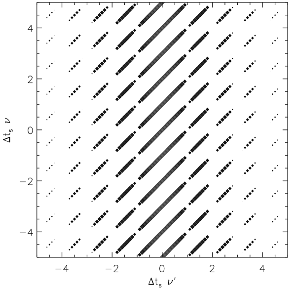
Figure 1.— Grey-scale representation of the “window function”, $\tilde{\mathcal{W}}$ (see eq. [2]), as a function of $\nu$ and $\nu^{\prime}$ for $\Delta t_{\rm s}=\Delta t_{\rm b}=1024$s and $\Delta t_{\rm o}=1024^{2}$s. Lighter shades of grey indicate higher values of $\tilde{\mathcal{W}}$. The function $\tilde{\mathcal{W}}$ reaches its maximum at $\nu^{\prime}=0$ with subsidiary peaks of decaying strength on both sides. As expected, the function $\tilde{\mathcal{W}}$ is periodic in $\nu$ with period $\Delta t_{\rm s}$.

As an aside, note that using the fact that the series of “$\mathrm{sinc}$” functions (weakly) converges to the Dirac delta, i.e.,

$$\lim_{\eta\rightarrow\infty}\eta\,\mathrm{sinc}^{2}(\pi\eta\nu)=\delta(\nu)~{},$$ (20)

it is not hard to show that, as expected, in the limit of an infinite and continuous observation the average of the observed power spectra tends to the underlying power spectrum, i.e.,

$$\lim_{\Delta t_{\rm o}\rightarrow\infty}\left(\lim_{\Delta t_{\rm s},\Delta t_{\rm b}\rightarrow 0}\Delta t_{\rm o}\langle P_{\rm o}(\nu)\rangle\right)=P(\nu)~{}.$$ (21)

Whenever a sampling pattern is applied, however, power at any given frequency will “leak” to other frequencies, and vice versa. The extent of this spectral leakage is fully characterized by the function $\tilde{\mathcal{W}}\left(\nu,\nu^{\prime};\Delta t_{\rm o},\Delta t_{\rm s},\Delta t_{\rm b}\right)$ (see Fig. 1).

3. Lorentzian Models for AGN Variability

In the previous section we showed how the average power spectrum inferred from a set of observations with the same sampling pattern differs from the underlying power spectrum. We can now write the average fractional rms that we would measure from such a set of observations as

$$\langle\sigma^{2}_{\rm rms}(\Delta t_{\rm o},\Delta t_{\rm s},\Delta t_{\rm b};M_{\rm BH})\rangle =$$

$$2\!\!\sum_{k=1}^{N/2-1}\!\!\langle P_{\rm o}(\nu_{k};M_{\rm BH})\rangle + \langle P_{\rm o}(\nu_{\rm Nyq};M_{\rm BH})\rangle~{},$$ (22)

where the function $\langle P_{\rm o}(\nu)\rangle$ is the power spectrum affected by sampling effects and is related to the underlying power spectrum, $P(\nu)$, according to equations (18) and (2). Equation (3) (together with eqs. [18] and [2]) must be at the core of any theoretical model addressing the functional form of the $\sigma^{2}_{\rm rms}$-${\thinspace M_{\rm BH}}$ correlation and considering the distorting effects imprinted in the data by the particular sampling pattern used to obtain the observed fractional rms (see also, O’Neill et al., 2005, where the case $\Delta t_{\rm b}=\Delta t_{\rm s}$ is discussed).

3.1. Advantages of Lorentzian Models

Inspired by the similarities shared by the the global timing properties of AGN and early observations of X-ray binaries, previous studies involving models of broad-band noise AGN power spectra are mostly based on underlying power spectra characterized by broken power laws. However, over the last decade, thanks to the timing capabilities of RXTE, it has been possible to study in great detail the X-ray variability of many galactic sources. It is now clear that the power spectra of X-ray binaries exhibit a rich morphology which, in general, cannot be adequately described in terms of broken power laws.

In many cases, it has been possible to obtain very good fits to the observed power spectra (of both neutron stars and black holes) using a small set of Lorentzians. It is important to point out that, whenever checked against each other, Lorentzian models usually yield better fits than power laws. Even when the fits are similarly good, the use of Lorentzians allows us to “follow” over time the different characteristic frequencies appearing in the power spectrum. This has been key to uncovering several correlations among the different broad-band noise components in X-ray binaries (Psaltis, Belloni, & van der Klis, 1999; Belloni, Psaltis, & van der Klis, 2002).

A typical Lorentzian model for the underlying power spectrum of an X-ray binary can be written as

$$P(\nu)=\sum_{l=1}^{N_{L}}L_{l}(\nu)=\sum_{l=1}^{N_{L}}\frac{r_{l}^{2}}{\pi}~{}\frac{\Delta_{l}}{\Delta^{2}_{l}+(\nu-\nu^{0}_{l})^{2}}~{},$$ (23)

where $N_{L}$ is the number of components, and $r_{l}$, $\Delta_{l}$, and $\nu^{0}_{l}$ stand for the fractional rms, the width, and the centroid frequency corresponding to each Lorentzian. Defined in this way, the power spectrum is “two sided” and therefore

$$r_{l}^{2}=\int_{-\infty}^{\infty}L_{l}(\nu)\,d\nu\,.$$ (24)

Although the data currently available for AGN might not allow yet for a clear distinction between power-law models and Lorentzian models, the underlying assumption of similar X-ray variability properties between AGN and X-ray binaries advocates for the development of a common phenomenological framework to study both kind of sources on the same footing. Motivated by this, we propose to use a small set of Lorentzians to model AGN power spectra.

3.2. Sampling Effects in Lorentzian Models

Broad-band noise components are usually characterized by ratios $\Delta_{l}/\nu^{0}_{l}\gg 1$ and, in most cases, it is a good approximation to set $\nu^{0}_{l}=0$ in equation (23) and describe the band-limited noise as a sum of zero-centered Lorentzians (Belloni, Psaltis, & van der Klis, 2002). Let us then assume an underlying broad-band noise power spectrum that can be described by a set of $N_{L}$ broad Lorentzians,

$$P(\nu)=\frac{1}{\pi}\sum_{l=1}^{N_{L}}r_{l}^{2}~{}\frac{\nu_{l}}{\nu^{2}_{l}+\nu^{2}}~{},$$ (25)

where $\nu_{l}$ is the HWHM of the $l^{th}$ zero-centered Lorentzian but also plays the role of a “peak frequency” in the $\nu P(\nu)$ vs. $\nu$ representation (see Fig. 2).

With the normalization chosen in equation (25), the variance of the light curves associated with the underlying power spectrum, $P(\nu)$, is indeed the fractional rms. In other words, the total fractional rms corresponding to the band-limited noise spectrum is just

$$\sigma^{2}_{\rm rms}=\int_{-\infty}^{\infty}\!\!P(\nu)\,d\nu=\sum_{l=1}^{N_{L}}r^{2}_{l}~{}.$$ (26)

This choice, together with the fact that the fractional rms is dimensionless, determines the units of all the quantities related to the power spectrum. In particular, the underlying (continuous) power spectrum has units of inverse frequency while its discrete counterpart (affected by sampling effects) is dimensionless. Because of this, the discrete values $P_{\rm o}(\nu_{k})$ must be multiplied by the observing time $\Delta t_{\rm o}$ in order to be compared with the underlying values $P(\nu_{k})$. This is also the reason for which the factor $\Delta t_{\rm o}$ appears explicitly in eq. (21).

Table 1Sample Lorentzian Model for the Power Spectrum

$L_{l}$	$r_{l}$	$\nu_{l}$[Hz]
$L_{1}(\nu)$	0.2	2.0 $\times 10^{-7}$
$L_{2}(\nu)$	0.2	1.5 $\times 10^{-6}$
$L_{3}(\nu)$	0.1	8.0 $\times 10^{-6}$

Note. — Parameters defining the sample power spectrum as a sum of three zero-centered broad Lorentzians. The fractional rms and the ratios between centroid frequencies for each Lorentzian are similar to those observed in Cyg X-1 (Pottschmidt et al., 2003), while the peak frequency of the lowest Lorentzian (i.e., $\nu_{1}$) is similar to the low frequency break observed in NGC 3783 (Markowitz et al., 2003).

Figure 2 shows a sample Lorentzian model for the broad-band noise power spectrum of a hypothetical AGN (see also Tab. 1). In this case, the fractional rms and the ratios between centroid frequencies for each Lorentzian are similar to those observed in Cyg X-1 (Pottschmidt et al., 2003), while the peak frequency of the lowest Lorentzian (i.e., $\nu_{1}$) is similar to the low frequency break of NGC 3783 (Markowitz et al., 2003).

Using equations (18) and (2) and the model power spectrum, $P(\nu)$, given by equation (25) we can write the average observed power spectrum, $\langle P_{\rm o}(\nu)\rangle$, as

$$\langle P_{\rm o}(\nu)\rangle=\sum_{l=1}^{N_{L}}\sum_{m=-\infty}^{\infty}I_{l,m}(\nu),$$ (27)

with

$$I_{l,m}(\nu) = \frac{r_{l}^{2}b_{l}}{\pi}\int_{-\infty}^{\infty}\!\!\mathrm{sinc}^{2}(\Delta x^{\prime})\,\frac{\mathrm{sinc}^{2}[a_{m}(\nu)-x^{\prime}]}{b_{l}^{2}+x^{\prime 2}}\,dx^{\prime}~{},$$

where we have defined the dimensionless variables

$$b_{l}=\pi\Delta t_{\rm o}\nu_{l} \quad\Delta=\Delta t_{\rm b}/\Delta t_{\rm o}\,,$$ ,

$$x^{\prime}=\pi\Delta t_{\rm o}~{}\nu^{\prime} \quad a_{m}(\nu)=\pi\Delta t_{\rm o}(\nu-\nu_{m})\,.$$ ,

This integral can be computed analytically in the complex plane using a slight modification of the residues theorem (see Appendix B for the details). The result is given by

$$I_{l,m}(\nu) = \frac{r_{l}^{2}b_{l}}{\Delta^{2}}\sum_{i=1}^{6}A^{i}_{l,m}(\nu),$$ (29)

$$A^{1}_{l,m}(\nu) = \frac{1-(1-\Delta)\cos(2\Delta a_{m})}{2a_{m}^{2}(a_{m}^{2}+b_{l}^{2})}~{},$$

$$A^{2}_{l,m}(\nu) = -\frac{\sin(2\Delta a_{m})(b_{l}^{2}+2a_{m}^{2})}{2a_{m}^{3}(a_{m}^{2}+b_{l}^{2})^{2}}~{},$$

$$A^{3}_{l,m}(\nu) = \frac{(b_{l}^{2}-a_{m}^{2})\cos(2a_{m})}{2(a_{m}^{2}+b_{l}^{2})^{2}b_{l}^{3}}~{}e^{-2b_{l}}\sinh^{2}(\Delta b_{l})~{},$$

$$A^{4}_{l,m}(\nu) = -\frac{a_{m}\sin(2a_{m})}{(a_{m}^{2}+b_{l}^{2})^{2}b_{l}^{2}}~{}e^{-2b_{l}}\sinh^{2}(\Delta b_{l})~{},$$

$$A^{5}_{l,m}(\nu) = \frac{(b_{l}^{2}-a_{m}^{2})}{2(a_{m}^{2}+b_{l}^{2})^{2}b_{l}^{3}}~{}e^{-\Delta b_{l}}\sinh(\Delta b_{l})~{},$$

$$A^{6}_{l,m}(\nu) = \frac{\Delta}{2a_{m}^{2}b_{l}^{2}}~{},$$

where we have omitted the frequency dependence of the coefficients $a_{m}(\nu)$ on the right hand sides of the expressions for $A^{i}_{l,m}(\nu)$. The symmetry property

$$A^{i}_{l,-m}(-\nu)=A^{i}_{l,m}(\nu)$$ (30)

reflects the fact that sampling effects do not affect the parity of the observed power spectrum, i.e., $\langle P_{\rm o}(\nu)\rangle=\langle P_{\rm o}(-\nu)\rangle$.

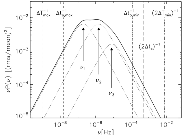
Figure 2.— The underlying power spectrum for a hypothetical AGN (solid line) modeled as a sum of three broad Lorentzians (dotted lines). The arrows indicate the positions of the peak frequencies (see Tab. 1). Vertical lines indicate the frequencies corresponding to the different timescales involved in the numerical experiment performed in §4.

It is important to summarize here what we have accomplished with equations (27) and (29). We have reduced the problem of accounting for the sampling effects caused by an arbitrary sampling pattern, $\{\Delta t_{\rm o},\Delta t_{\rm s},\Delta t_{\rm b}\}$, in any broad-band noise power spectrum that can be decomposed into a sum of zero-centered Lorentzians, to evaluating a simple sum. In practice, the sum in equation (27) converges extremely fast and it is necessary to add only a few (order of five) terms at any given frequency. This makes the process of accounting for sampling effects in Lorentzian models highly efficient if the aim is to run a grid of models to contrast them against observations in order to constrain the functional form of the underlying power spectrum. We stress that, if the underlying power spectrum is given by equation (25), the average $\langle P_{\rm o}(\nu)\rangle$ calculated according to equations (27) and (29) provides the value to which Monte Carlo simulations, devised to account for the sampling effects imprinted by the sampling pattern $\{\Delta t_{\rm o},\Delta t_{\rm s},\Delta t_{\rm b}\}$, will converge. In the next section we show that this is indeed the case.

4. Contrasting the Analytical Prediction to Monte Carlo Simulations

The aim of this section is two-fold. First, we want to test how well our analytical prediction is able to account for the distortions suffered by the underlying power spectrum due to sampling effects. Second, we would like to obtain an idea about how important of an effect one is neglecting when calculating the rms variability using equation (1) instead of (3) for a sampling pattern typical of AGN observations. In order to do this, we performed a series of numerical experiments calculating independently both sides of equation (3) assuming the model power spectrum characterized by the three broad Lorentzians shown in Table 1 (see also Fig. 2).

In order to test the validity of equation (3), we need to provide a good representation of the ‘infinite” and “continuous” light curve, $C(t)$, associated with the underlying power spectrum, $P(\nu)$. Then we can segment, bin, and sample this “real” light curve according to the sampling pattern $\{\Delta t_{\rm o},\Delta t_{\rm s},\Delta t_{\rm b}\}$, obtain a set of time series $\{C_{o}(t_{n})\}$, and calculate the rms amplitude, $\sigma^{2}_{\rm rms}$, associated with each sampled light curve as

$$\sigma^{2}_{\rm rms}=\frac{1}{N-1}\sum_{n=0}^{N-1}|C_{0}(t_{n})-\bar{C}_{0}|^{2}\,,$$ (31)

where $N=\Delta t_{\rm o}/\Delta t_{\rm s}$ and $\bar{C_{0}}$ is the average corresponding to the particular time series $\{C_{o}(t_{n})\}$. The mean value in equation (3), $\langle\sigma^{2}_{\rm rms}\rangle$, can then obtained by averaging over several “observed” light curves with the same sampling pattern.

Of course, a numerical representation of the “real” light curve $C(t)$ will still be given by a discrete set of values $\{C(t_{l})\}$, much in the same way as we can only evaluate the underlying (continuous) power spectrum at a finite number of frequencies $\{P(\nu_{k})\}$. The way of doing this is to consider a minimum frequency, $\nu_{\rm min}$, and a maximum frequency, $\nu_{\rm max}$, such that the contributions to the rms variability from power outside the range $[\nu_{\rm min},\nu_{\rm max}]$ is negligible, i.e.,

$$\int_{0}^{\nu_{\rm min}}P(\nu)\,d\nu\,,\int_{\nu_{\rm max}}^{\infty}P(\nu)\,d\nu\,\ll\int_{\nu_{\rm min}}^{\nu_{\rm max}}P(\nu)\,d\nu~{}.$$ (32)

In the case of the model under consideration this can be accomplished by choosing $\nu_{\rm min}\ll\nu_{1}$ and $\nu_{\rm max}\gg\nu_{3}$. Note that this is a much stronger condition than requiring that $\nu_{\rm min}\ll 1/\Delta t_{\rm o}$ and/or $\nu_{\rm max}\gg 1/2\Delta t_{\rm s}$ for the particular sampling pattern under consideration. These conditions over $\nu_{\rm min}$ and $\nu_{\rm max}$ are necessary but not sufficient.

For all practical purposes, the time series $\{C(t_{l})\}$ obtained in this way can be considered as an accurate representation of $C(t)$ in the sense that the power spectrum estimated from it will not be noticeably affected by sampling effects. Note that, the set of values $\{P_{\rm o}(\nu_{k})\}$ corresponds to one given realization of the stochastic process and, therefore, in general, it does not coincide with the values of the underlying power spectrum $\{P(\nu_{k})\}$ at any given frequency even in this case! However, the lack of sampling effects is noticed in the absence of the trends that would be introduced by red noise leakage and/or aliasing inside the range $[\nu_{\rm min},\nu_{\rm max}]$.

In order to set up the numerical experiment, we generate the “continuous” light curve by setting $\nu_{\rm min}=1/\Delta T_{\rm max}=9.3\times 10^{-10}$Hz (i.e., $\Delta T_{\rm max}=2^{30}$s or roughly 36 yrs) and $\nu_{\rm max}=\nu_{\rm Nyq}=1/(2\Delta T_{\rm min})=7.8\times 10^{-3}$Hz ($\Delta T_{\rm min}=64$s). This yields $N\equiv\Delta T_{\rm max}/\Delta T_{\rm min}=2^{24}\simeq 10^{7}$ initial “data” points. The frequencies corresponding to $\nu_{\rm min}$ and $\nu_{\rm max}$ are indicated with vertical lines (dotted and triple-dot-dashed line, respectively) in Figure 2. The conditions stated in equation (32) are clearly satisfied.

Figure 3.— The square of the fractional rms, $\sigma^{2}_{\rm rms}$, associated with the model power spectrum, $P(\nu)$, as a function of the observation time $\Delta t_{\rm o}$ calculated in three different ways. Filled circles: results obtained from Monte Carlo simulations. Solid line: the analytical prediction given by the right hand side of eq. (3). Dashed line: results obtained by neglecting sampling effects, i.e., using eq. (1). In this case, the binning time is equal to the sampling time.

Under our current set of assumptions, we can generate the time series $\{C(t_{l})\}$, with $t_{l}=l\Delta T_{\rm min}$ and $l=0,...,N-1$ from the set $\{P(\nu_{k})\}$, with $\nu_{k}=k/\Delta T_{\rm max}$ and $k=-N/2+1,...,N/2$, as

$$C(t_{l})=\!\!\sum_{k=N/2-1}^{N/2}\!\!c_{k}~{}e^{2\pi i\nu_{k}t_{l}}~{},$$ (33)

with

$$c_{k}=\sqrt{\frac{P(\nu_{k})}{\Delta T_{\rm max}}}~{}e^{2\pi i\phi(\nu_{k})}~{}.$$ (34)

In order to generate a true realization of the stochastic process with underlying power spectrum $P(\nu)$, the amplitudes under the square root in equation (34) must satisfy $P(\nu_{k})=P(-\nu_{k})$ and be drawn from a $\chi^{2}$ distribution with two degrees of freedom for all $\nu_{k}\neq\nu_{\rm Nyq}$ and from a $\chi^{2}$ distribution with one degree of freedom for $\nu_{\rm Nyq}$. Alternatively, this can also be done by generating two normally distributed random variables, multiplying them by $[P(\nu_{k})/\Delta T_{\rm max}]^{1/2}$, and using them to define the real and imaginary parts of the discrete Fourier Transform given by the set $\{c_{k}\}$(see, e.g., Timmer & König, 1995, for more details). Moreover, in order to ensure that the generated light curve is real, the set of random phases $\{\phi(\nu_{k})\}$ must satisfy $\{\phi(-\nu_{k})\}=\{-\phi(\nu_{k})\}$ for all $k\neq 0,N/2$ and $\phi(0)=0$ or $\pi$, as well as $\phi(\nu_{\rm Nyq})=0$ or $\pi$.

Note that, by construction, if we were to take the discrete Fourier Transform of the set $\{C(t_{l})\}$ and calculate $\{P(\nu_{k})\}=\Delta T_{\rm max}\{|c_{k}|^{2}\}$ then sampling effects would be negligible in the range $[\nu_{\rm min},\nu_{\rm max}]$. For all practical purposes then, the set $\{C(t_{l})\}$ can be thought of as an accurate representation of the “infinite” and “continuous” light curve $C(t)$.

We can now define a sampling pattern, $\{\Delta t_{\rm o},\Delta t_{\rm s},\Delta t_{\rm b}\}$, and do everything we would do if we were recording a time series from the continuous light curve $C(t)$. In order to be able to compute an average value for the rms variability we divided the original light curve of duration $\Delta T_{\rm max}$ in 16 light curves of duration $\Delta t_{\rm o,max}=2^{26}$s. We also defined the duration of each time bin as $\Delta t_{\rm b}=1024$s, as a representative value used in AGN observations. Note that this value of $\Delta t_{\rm b}$ will include $16$ discrete points of the original time series $\{C(t_{l})\}$. To simplify the discussion, in what follows, we will consider a continuous monitoring campaign, i.e., $\Delta t_{\rm s}=\Delta t_{\rm b}$ (we consider a case in which $\Delta t_{\rm s}>\Delta t_{\rm b}$ in the next section).

We calculated the fractional rms variability for each light curve of duration $\Delta t_{\rm o,max}$ according to equation (31) and obtained the average value that we took as the left hand side of equation (3). We repeated this procedure defining an increasingly larger number of segmented (independent) light curves of duration $\Delta t_{{\rm o}}=2^{-n}\Delta t_{\rm o,max}$ with $n=0,...,13$. Figure 3 shows the values of $\langle\sigma^{2}_{\rm rms}\rangle$ as a function of the observing time, $\Delta t_{{\rm o}}$. The analytical prediction (i.e., the right hand side of eq. [3]) is shown with a solid line, the filled circles represent the average values $\langle\sigma^{2}_{\rm rms}\rangle$ obtained from the light curves generated with the Monte Carlo simulations, and the dashed line shows the value of $\sigma^{2}_{\rm rms}$ as obtained using equation (1).

Table 2Sampling Effects on the Fractional RMS

n	$\Delta t_{\rm o}/\Delta t_{\rm s}$	$\sigma^{2}_{\rm rms,WA}/\sigma^{2}_{\rm rms,NS}$
3	8192	$\sim 10.00\,\%$
4	4096	$\sim 20.00\,\%$
9	128.0	$\sim 100.0\,\%$
12	16.00	$\sim 200.0\,\%$

Note. — Comparison between the fractional rms obtained considering and neglecting sampling effects as a function of the ratio between the observing and the sampling times. The symbols $\sigma^{2}_{\rm rms,WA}$ and $\sigma^{2}_{\rm rms,NS}$ denote the fractional rms derived from the “windowed” and “aliased” power spectrum (eq. [3]), and the value obtained when sampling effects are neglected (eq. [1]).

It is important to stress that we have not adjusted the normalization of any quantity when plotting the different variances in Figure 3. The convergence of the different fractional amplitudes for large values of $\Delta t_{\rm o}$ to the total rms amplitude of the model (i.e., $\sigma^{2}_{\rm rms}=0.09$) indicates that sampling effects become negligible when the harmonic content of the observed light curve is a good representation of the underlying power spectrum. This is in agreement with equation (21). As the observation time decreases, the fractional rms, as calculated according to equation (1), underestimates the values obtained from either side of equation (3), i.e., the fractional rms obtained from either the analytical result or the Monte Carlo simulations, by a factor of up to $200\%$ (see Tab. 2 for details).

In the previous numerical experiments, the fractional rms was obtained directly from the light curves without the need of deriving the power spectra associated with them. Figure 4 shows the average power spectra derived from the Monte Carlo simulations (filled circles) for the case $\Delta t_{\rm s}=\Delta t_{\rm b}=1024$s and $\Delta t_{\rm o}=65536$s (corresponding to $n=10$) together with the corresponding analytical result (open circles) derived using equations (27)-(29). The distorting effects suffered by the power spectrum derived from the finite and discrete light curves with respect to the underlying power spectrum (solid line) are evident. This remarkable agreement between the averaged observed power spectra derived analytically and using the simulated light curves is the reason behind the coincidence of the associated fractional variability amplitudes in Figure 3.

As a corollary, we note that, by adopting a Lorentzian model for the underlying power spectrum, the results from §3.2 can be used to test Monte Carlo simulations when the frequencies are assumed to be uncorrelated.

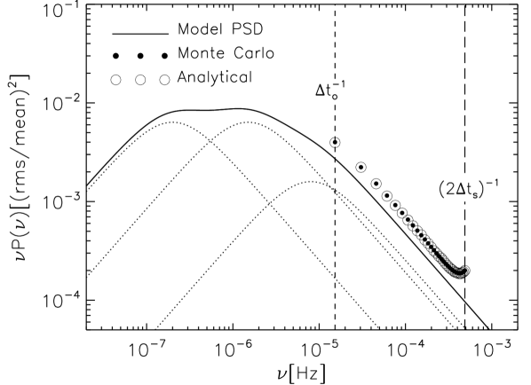
Figure 4.— Sampling distortions suffered by the model power spectrum defined in Tab. 1 (solid line), as obtained from calculating the (average) discrete power spectrum associated with the light curves generated via Monte Carlo simulations (filled circles), and as predicted by our analytical calculation (open circles). The sampling pattern is defined by $\Delta t_{\rm o}=65536$s and $\Delta t_{\rm s}=\Delta t_{\rm b}=1024$s. Note that the discrete values $P_{\rm o}(\nu_{k})$ must be multiplied by $\Delta t_{\rm o}$ in order to be compared with the underlying values $P(\nu_{k})$.

5. Discussion

This is the first paper in a series aimed to exploit the similarities observed in the X-ray timing properties of AGN and X-ray binaries in order to measure the masses of supermassive black holes using X-ray variability.

The idea of using X-ray variability to obtain the masses of AGN by comparing their timing properties to those of X-ray binaries is not new (Hayashida et al., 1998; Lu & Yu, 2001; Czerny et al., 2001; Bian & Zhao, 2003; Papadakis, 2004; Nikolajuk, Papadakis, & Czerny, 2004). A key assumption necessary for this procedure to provide reliable results is that the processes driving the variability, and therefore the associated underlying power spectra, are similar. Although the data currently available for some AGN is encouraging in this respect (Uttley et al., 2002; Markowitz et al., 2003), so far there have been no attempts of describing the timing properties of both kind of objects on the same footing. Motivated by the latest timing studies carried out on a number of galactic black-hole candidates, we have proposed to model the broad-band noise spectra of AGN in the same way that has been successful with many X-ray binaries, i.e., as a sum of Lorentzian components.

A particular concern when connecting theoretical models of broad-band noise X-ray variability with observations is that sampling effects (especially red noise leakage) are much more important for AGN than for X-ray binaries. In the last few years it has become evident that in order to derive reliable power-spectra estimates from the observations it is imperative to account for these sampling effects (Uttley et al., 2002). Less attention has been paid, however, to the effects that sampling has on the connection between the underlying power spectrum and the rms variability (but see O’Neill et al., 2005).

In order to illustrate the importance of this latter issue, let us assume a hypothetical Lorentzian model resembling the underlying power spectrum obtained for NGC 3783. Markowitz et al. (2003) found that a reasonable description of this power spectrum can be obtained by a double broken power-law model with characteristic (“low” and “high”) break frequencies given by $\nu_{l}=2.00\times 10^{-7}$Hz and $\nu_{h}=3.98\times 10^{-6}$Hz, and an amplitude $A\simeq 0.01$ (the corresponding power-law slopes at low and intermediate frequencies were fixed to 0 and -1 respectively and the best fit at high frequencies is consistent with a power-law of -2). A Lorentzian model to describe this underlying power spectrum could be obtained using two Lorentzian components (dotted lines in Fig. 5) as follows

$$P(\nu)=\frac{r_{1}^{2}}{\pi}\frac{\nu_{1}}{\nu_{1}^{2}+\nu^{2}}+\frac{r_{2}^{2}}{\pi}\frac{\nu_{2}}{\nu_{2}^{2}+\nu^{2}}~{},$$ (35)

where we have denoted the characteristic frequencies as $\nu_{1}=\nu_{l}$ and $\nu_{2}=\nu_{h}$. We assume here that $r_{1}^{2}=r_{2}^{2}=0.075$ so that the peak amplitude of each Lorentzian in $\nu P(\nu)$ space is roughly 0.01. As an aside, we note that the ratio of frequencies derived from observations is such that these two Lorentzians (with the same amplitude) lead naturally to a flat slope in the $\nu P(\nu)$ representation. This feature is observed in several X-ray binaries, i.e., in many cases the frequencies and amplitudes of the different broad Lorentzians are such that the overall shape of the (underlying) power spectrum resembles a $1/\nu$ power law over a wide range in frequencies (Belloni, Psaltis, & van der Klis, 2002).

Table 3Typical Sampling Patterns for AGN

Term Type	$\Delta t_{\rm o}$	$\Delta t_{\rm s}$	$\Delta t_{\rm b}$	$\sigma^{2}_{\rm rms,WA}/\sigma^{2}_{\rm rms,NS}$
Long	4.27$\times$266 d	4.27 d	1024.8 s	$\sim 78\,\%$
Medium	3.20$\times$151 h	3.20 h	1152.0 s	$\sim 32\,\%$
Short	2000$\times$84 s	2000 s	2000.0 s	$\sim 77\,\%$

Note. — The sampling patterns for short-term observations are typical of ASCA, Chandra, and/or XMM-Newton. The values of $\{\Delta t_{\rm o},\Delta t_{\rm s},\Delta t_{\rm b}\}$ for long-term observations are more representative of RXTE observations. The meaning of the symbols $\sigma^{2}_{\rm rms,WA}$ and $\sigma^{2}_{\rm rms,NS}$ is the same as in Tab. 2.

Let us now suppose that we “observe” the model defined by equation (35) according to the different sampling patterns involved in the various types (long-, medium- and short-term) of monitoring campaigns designed to observe NGC 3783 (see Tab. 3). By calculating the rms variability according to equation (1), ($\sigma^{2}_{\rm rms,NS}$, i.e., not considering sampling effects), and equation (3), ($\sigma^{2}_{\rm rms,WA}$, i.e., when the rms variability is calculated based on the “windowed” and “aliased” power spectrum) we can study how important are the consequences of neglecting sampling effects. The last column in Table 3 shows the ratio of these two variances for the different types of sampling patterns. For the adopted power spectrum, neglecting sampling effects can lead us to underestimate the observed value of the rms variability by up to $80\%$. These differences can also be understood by looking at the sampling effects directly in the power spectrum. Figure 5 shows the “observed” power spectra that we would obtain from monitoring a source with an underlying power spectrum given by equation (35), according to the sampling patterns listed in Table 3.

It is not straightforward to see how these differences in the variances will affect the mass estimates derived from a theoretical model of the $\sigma^{2}_{\rm rms}$-${\thinspace M_{\rm BH}}$ correlation. This will depend, of course, upon the functional form of the $\sigma^{2}_{\rm rms}$-${\thinspace M_{\rm BH}}$ correlation itself. We note here that a difference in rms variability will likely be amplified when translated into a difference in mass. This is because the observed fractional rms is a rather flat function of black-hole mass. Indeed, for a large number of AGN the fractional rms is known to vary between $30\%$ and $40\%$ in long-term observations and between $2\%$ and $30\%$ in short-term observations, over almost four orders of magnitude in black-hole mass (Markowitz et al., 2003).

This flattening of the observed $\sigma^{2}_{\rm rms}$-${\thinspace M_{\rm BH}}$ correlation for larger observation times suggest that, for the sake of deriving masses, short observations should be favored over long term monitoring campaigns. This is, of course, when sampling effects (in particular red noise leakage) will affect the most the connection between the model power spectrum and the observed fractional rms variability. For this reason, it is vital to incorporate sampling effects in theoretical models that aim to estimate black-hole masses via the $\sigma^{2}_{\rm rms}$-${\thinspace M_{\rm BH}}$ correlation if they rely on a parametrization of the underlying AGN power spectrum in terms of ${\thinspace M_{\rm BH}}$.

Figure 5.— Illustration of the distorting effects suffered by the underlying power spectrum, $P(\nu)$ (solid lines), modeled with two Lorentzian components (dotted lines, see eq. [35]) when it is “observed” according to different sampling patterns (see Tab. 3). The different symbols, filled diamonds, open circles, and filled triangles, indicate the “windowed” and “aliased” power spectra that would be derived from long-, medium-, and short-term observations respectively.

It is evident from Figure 5 that the effects of spectral leakage have to be considered when (continuous) model power spectra are to be compared against (average) power spectra obtained from observed time series. State of the art techniques to “convolve” the models with the observation sampling patterns currently involve sophisticated Monte Carlo methods. These simulations are crucial once the “best fit model” has been found in order to assess the confidence levels associated with the best fit parameters. The high numerical costs associated with this type of simulations, however, usually rules in favor of mathematical models that can be described with a low number of free parameters which might not allow enough freedom to properly describe the data.

The proposed Lorentzian models for broad-band noise variability offer a tremendous advantage in this sense. In the measure that the available data allows it, the gain in computational speed obtained by using analytical expressions to account for sampling effects could be used to explore parameter spaces of higher dimensions. This will play in favor of more realistic mathematical models as it is the case for X-ray binaries.

Appendix A Average Over Realizations

In §2 we stated that the average over ensembles of the quantity $\langle\tilde{C}(\nu^{\prime})\tilde{C}^{*}(\nu^{\prime\prime})\rangle$ was related to the underlying power spectrum of a stationary stochastic process via equation (17). Here, we provide a brief demonstration of this statement.

By definition, the average $\langle\tilde{C}(\nu^{\prime})\tilde{C}^{*}(\nu^{\prime\prime})\rangle$ can be written in terms of the corresponding average in the time domain as

$$\langle\tilde{C}(\nu^{\prime})\tilde{C}^{*}(\nu^{\prime\prime})\rangle=\int_{-\infty}^{\infty}\int_{-\infty}^{\infty}\langle C(t^{\prime})C^{*}(t^{\prime\prime})\rangle~{}e^{-i2\pi\nu^{\prime}t^{\prime}}~{}e^{i2\pi\nu^{\prime\prime}t^{\prime\prime}}dt^{\prime}dt^{\prime\prime}~{},$$ (A1)

where $C(t)$ corresponds to the inverse Fourier Transform of $\tilde{C}(\nu)$. For a continuous process with zero mean, the quantity $\langle C(t^{\prime})C^{*}(t^{\prime\prime})\rangle$ is the correlation function $\xi(t^{\prime},t^{\prime\prime})$. Furthermore, if the process is stationary, the expectation value $\langle C(t^{\prime})C^{*}(t^{\prime\prime})\rangle$ can only be a function of the time difference $t^{\prime}-t^{\prime\prime}$ and, therefore,

$$\langle\tilde{C}(\nu^{\prime})\tilde{C}^{*}(\nu^{\prime\prime})\rangle=\int_{-\infty}^{\infty}\int_{-\infty}^{\infty}\xi(t^{\prime}-t^{\prime\prime})~{}e^{-i2\pi\nu^{\prime}t^{\prime}}~{}e^{i2\pi\nu^{\prime\prime}t^{\prime\prime}}~{}dt^{\prime}dt^{\prime\prime}~{}.$$ (A2)

Defining $\tau=t^{\prime}-t^{\prime\prime}$ and $\tilde{\tau}=t^{\prime}$, we can write

$$\langle\tilde{C}(\nu^{\prime})\tilde{C}^{*}(\nu^{\prime\prime})\rangle = \int_{-\infty}^{\infty}\int_{-\infty}^{\infty}\xi(\tau)e^{-i2\pi\nu^{\prime}\tilde{\tau}}~{}e^{i2\pi\nu^{\prime\prime}(\tilde{\tau}-\tau)}d\tau d\tilde{\tau}~{},$$ (A3)

$$= \int_{-\infty}^{\infty}\xi(\tau)e^{-i2\pi\nu^{\prime\prime}\tau}~{}d\tau\int_{-\infty}^{\infty}e^{-i2\pi(\nu^{\prime}-\nu^{\prime\prime})\tilde{\tau}}~{}d\tilde{\tau}~{},$$ (A4)

$$= F[\xi](\nu^{\prime\prime})~{}\delta(\nu^{\prime}-\nu^{\prime\prime})~{},$$ (A5)

where the quantity $F[\xi](\nu^{\prime\prime})$ stands for the Fourier Transform of the autocorrelation function, which is the underlying power spectrum, $P(\nu^{\prime\prime})$. In this way, we obtain the result quoted in equation (17), i.e.,

$$\langle\tilde{C}(\nu^{\prime})\tilde{C}^{*}(\nu^{\prime\prime})\rangle=P(\nu^{\prime\prime})~{}\delta(\nu^{\prime}-\nu^{\prime\prime})\,.$$ (A6)

Appendix B Contour Integral

Figure 6.— The integration paths in the upper ($\Gamma_{+}$) and lower ($\Gamma_{-}$) halves of the complex plane used to calculate the coefficients $I_{l,m}(\nu)$ in equation (B1). The functions $f_{p}^{\pm}$ defined in equation (B) decay exponentially over $\Gamma_{\pm}$ for ${\mathcal{I}m}(z)\gtrless 0$, respectively, when the radii of the contours tend to infinity.

In §3.2 we presented an analytic expression for the coefficients $I_{l,m}(\nu)$ involved in the calculation of the average power spectrum affected by sampling effects according to the sampling pattern $\{\Delta t_{\rm o},\Delta t_{\rm s},\Delta t_{\rm b}\}$. Here, we outline how to obtain them.

The integral defining the coefficients $I_{l,m}(\nu)$, i.e.,

$$I_{l,m}(\nu) = \frac{r_{l}^{2}b_{l}}{\pi}\int_{-\infty}^{\infty}~{}\frac{\sin^{2}(\Delta x^{\prime})}{(\Delta x^{\prime})^{2}}~{}\frac{\sin^{2}[a_{m}(\nu)-x^{\prime}]}{[a_{m}(\nu)-x^{\prime}]^{2}}~{}\frac{dx^{\prime}}{b_{l}^{2}+x^{\prime 2}}~{},$$ (B1)

exists and is real for any non-zero value of $b_{l}$ and any finite value of $\Delta$, and $a_{m}(\nu)$. A convenient way to calculate its value is to allow the variable $x^{\prime}$ to be complex and compute $I_{l,m}(\nu)$ as a contour integral in the complex plane by choosing suitable integration paths. The idea, as usual, is to find a contour of integration that contains the real axis and close it conveniently in such a way that the imaginary contribution vanishes when the real part of the contour extends from $-\infty$ to $\infty$. In order to do so, it is necessary to rewrite the sines in terms of complex exponentials that decay in the upper or lower half of the complex plane depending on their sign. We can rewrite equation (B1) as

$$I_{l,m}(\nu) = \frac{r_{l}^{2}b_{l}}{16\pi}\sum_{p=1}^{3}\sum_{\pm}\int_{-\infty}^{\infty}\frac{f^{\pm}_{p}(z^{\prime})}{(\Delta z^{\prime})^{2}[a_{m}(\nu)-z^{\prime}]^{2}}~{}\frac{dz^{\prime}}{b_{l}^{2}+z^{\prime 2}}~{}.$$ (B2)

where the functions $f_{p}^{\pm}$ for $p=1,2,3$ are given by

$$f^{\pm}_{1}(z) = (e^{2i\Delta z}-1)~{}e^{\pm i[2(z-a_{m})]}~{},$$

$$f^{\pm}_{2}(z) = (e^{-2i\Delta z}-1)~{}e^{\pm i[2(z-a_{m})]}~{},$$

$$f^{\pm}_{3}(z) = 2(1-e^{\pm 2i\Delta z})~{}.$$ (B3)

Note that because $\Delta=\Delta t_{\rm b}/\Delta t_{\rm o}<1$, the functions $f_{p}^{+}$ and $f_{p}^{-}$, for $p=1,2,3$, decay exponentially in the upper and lower halves of the complex plane respectively. A minor complication arises because the integrand presents (simple) poles on the real axis, i.e., at $z_{o}=0$ and $z_{m}=a_{m}(\nu)$, so some care is required when choosing the contours of integration in either half. Figure 6 shows a possible way of choosing two closed paths. The contours $\Gamma_{\pm}$ are adequate to calculate the integrals containing the functions $f_{p}^{\pm}$, respectively. Using a slight modification of the residues theorem (see, e.g., Marsden & Hoffman, 1999) we can calculate the integrals in equation (B2) to obtain

$$I_{l,m}(\nu) = \frac{r_{l}^{2}b_{l}}{16\pi}\sum_{p=1}^{3}\sum_{\pm}\pm 2\pi i{\mathcal{R}es}(f_{p}^{\pm},\pm b_{l})\pm\pi i{\mathcal{R}es}(f_{p}^{\pm},0)\pm\pi i{\mathcal{R}es}[f_{p}^{\pm},a_{m}(\nu)]~{},$$ (B4)

where ${\mathcal{R}es}(f,z)$ stands for the residue of the function $f$ evaluated at the (simple) pole $z$. Note that the signs in this equation properly take care of the negative orientation of the contour $\Gamma_{-}$. After some lengthy, but otherwise straightforward, algebra to regroup similar terms, equation (B4) yields the result quoted in equation (29).

References

- Belloni & Hasinger (1990) Belloni, T., & Hasinger, G. 1990, A&A, 227, L33
- Belloni, Psaltis, & van der Klis (2002) Belloni, T., Psaltis, D., & van der Klis, M. 2002, ApJ, 572, 392
- Bian & Zhao (2003) Bian, W., & Zao, Y. 2003, MNRAS, 343, 164
- Czerny et al. (2001) Czerny, B., Nikolajuk, M., Piasecki, M., & Kuraszkiewicz, J. 2001, MNRAS, 325, 865
- Deeming (1975) Deeming, T. J. 1975, Ap&SS, 36, 137
- Edelson & Nandra (1999) Edelson, R., & Nandra, K. 1999, ApJ, 514, 682
- Hayashida et al. (1998) Hayashida, K., Miyamoto, S., Kitamoto, S., Negoro, H., & Inoue, H. 1998, ApJ, 500, 642
- Lu & Yu (2001) Lu, Y., & Yu, Q. 2001, MNRAS, 324, 653
- Mauche (2002) Mauche, C. W. 2002, ApJ, 580, 423
- Marsden & Hoffman (1999) Marsden, J. E., & Hoffman, M. J. 1999, Basic Complex Analysis, Third Edition. (New York: W. H. Freeman and Company)
- Marshall, Warwick, & Pounds (1981) Marshall, H., Warwick, R., & Pounds, K. 1981, MNRAS, 194, 987
- Markowitz & Edelson (2001) Markowitz, A., & Edelson, R. 2001, ApJ, 547, 684
- Markowitz & Edelson (2004) ———. 2004, ApJ, 617, 939
- Markowitz et al. (2003) Markowitz, A., et al. 2003, ApJ, 593, 96
- McHardy et al. (2004) McHardy, I. M., Papadakis, I. E., Uttley, P., Page, M. J., & Mason, K. O. 2004, MNRAS, 348, 783
- McHardy et al. (2005) McHardy, I. M., Gunn, K. F., Uttley, P., & Goad, M. R., 2005, MNRAS, 359, 1469
- Miyamoto et al. (1994) Miyamoto, S., Kitamoto, S., Iga, S., Hayashida, K., & Terada, K. 1994, ApJ, 435, 398
- Morse & Feshbach (1953) Morse, P. M., & Feshbach, H. 1953, Methods of Theoretical Physics, Vol. 1. (New York: McGraw Hill)
- Mushotzky, Done, & Pounds (1993) Mushotzky, R. F., Done, C., & Pounds, K. A. 1993, ARA & A, 31, 717
- Nandra et al. (1997) Nandra, K., George, I. M., Mushotzky, R. F., Turner, T. J., & Yaqoob, T. 1997, ApJ, 476, 70
- Nikolajuk, Papadakis, & Czerny (2004) Nikolajuk, M., Papadakis, I. E., & Czerny, B. 2004, MNRAS, 350, L26
- Nowak (2000) Nowak, M. A. 2000, MNRAS, 318, 361
- O’Neill et al. (2005) O’Neill, P. M., Nandra, K., Papadakis, I. E., & Turner, T. J. 2005, MNRAS, 358, 1405
- Papadakis (2004) Papadakis, I. E. 2004, MNRAS, 348, 207
- Pottschmidt et al. (2003) Pottschmidt, K., et al. 2003, A&A, 407, 1039
- Priestley (1989) Priestley, M. B. 1989, Spectral Analysis and Time Series. (London: Academic Press Limited)
- Press et al. (1992) Press, W. H., Teukolsky, S. A., Vetterling, W. T., & Flannery, B. P. 1992, Numerical Recipes in FORTRAN: The Art of Scientific Computing (Cambridge: Cambridge Univ. Press)
- Psaltis, Belloni, & van der Klis (1999) Psaltis, D., Belloni, T., & van der Klis, M. 1999, ApJ, 520, 262
- Sunyaev & Revnivtsev (2000) Sunyaev, R., & Revnivtsev, M. 2000, A&A, 358, 617
- Turner et al. (1999) Turner, T. J., George, I. M., Nandra, K., & Turcan, D. 1999, ApJ, 524, 667
- Timmer & König (1995) Timmer, J., & König, M. 1995, A&A, 300, 707
- Uttley & McHardy (2004) Uttley, P., & McHardy, I. M. 2004, PThPS, 155, 170
- Uttley et al. (2002) Uttley, P., McHardy, I. M., & Papadakis, I. E. 2002, MNRAS, 332, 231
- van der Klis (1989) van der Klis, M. 1989, in Timing Neutron Stars, eds. H. Ögelman, & E. P. J. van den Heuvel (Dordrecht: Kluwer Academic Publishers)
- van der Klis (1994) ———. 1994, ApJS, 92, 511
- van der Klis (2005) ———. 2005, in Compact stellar X-ray Sources, eds. W. H. G. Lewin, & M. van der Klis, (Cambridge: Cambridge University Press)
- Wijnands & van der Klis (1999) Wijnands, R., & van der Klis, M. 1999, ApJ, 520, 262
- Warner & Woudt (2002) Warner, B., & Woudt, P. A. 2002, MNRAS, 335, 84
- Woo & Urry (2002) Woo, J. H., & Urry, C. M. 2002, ApJ, 579, 530