Angular momentum losses and the orbital period distribution of cataclysmic variables below the period gap: effects of circumbinary disks
Abstract
The population synthesis of cataclysmic variable binary systems at short orbital periods ( hrs) is investigated. A grid of detailed binary evolutionary sequences has been calculated and included in the simulations to take account of additional angular momentum losses beyond that associated with gravitational radiation and mass loss, due to nova outbursts, from the system. As a specific example, we consider the effect of a circumbinary disk to gain insight into the ingredients necessary to reproduce the observed orbital period distribution. The resulting distributions show that the period minimum lies at about 80 minutes with the number of systems monotonically increasing with increasing orbital period to a maximum near 90 minutes. There is no evidence for an accumulation of systems at the period minimum which is a common feature of simulations in which only gravitational radiation losses are considered. The shift of the peak to about 90 minutes is a direct result of the inclusion of systems formed within the period gap. The period distribution is found to be fairly flat for orbital periods ranging from about 85 to 120 minutes. The steepness of the lower edge of the period gap can be reproduced, for example, by an input of systems at periods near 2.25 hrs due to a flow of cataclysmic variable binary systems from orbital periods longer than 2.75 hrs.
The good agreement with the cumulated distribution function of observed systems within the framework of our model indicates that the angular momentum loss by a circumbinary disk or a mechanism which mimics its features coupled with a weighting factor to account for selection effects in the discovery of such systems and a flow of systems from above the period gap to below the period gap are important ingredients for understanding the overall period distribution of cataclysmic variable binary systems.
1 Introduction
Amongst the observed properties of cataclysmic variable binary systems (CVs), the most reliably determined quantity is the orbital period. The distribution of these orbital periods is fundamental, and theoretical interpretation of its features requires knowledge of the formation and evolution of these systems. Despite the increase in the number of CVs with determined orbital period to more than 500 systems as a result of their discovery in optical surveys in the last decade, their orbital period distribution has continued to defy explanation. This has, in part, been due to our poor knowledge of the theoretical description of the angular momentum loss processes which are essential for understanding the evolution of these systems.
The major uncertainty stems from our lack of a fundamental theory for angular momentum loss associated with a magnetically coupled stellar wind. The form of magnetic braking that has been the basis of most previous works on the evolution of CVs traces back to the pioneering work of Skumanich (1972), who determined that the stellar rotational velocity of slowly rotating main sequence G type stars varied inversely proportional to the square root of its age. Donor stars in CVs, however, typically rotate much more rapidly (with rotation periods hrs) than single stars of the same spectral type, and the implicit assumption that the form of angular momentum loss derived for slow rotation can be extrapolated and applied to fast rotators is without substantiation. Based on theoretical grounds, a departure from this form is expected since the acceleration of the stellar wind changes from thermally driven to centrifugally driven as the rotation speed increases. It is now generally accepted that the angular momentum loss rate from rapidly rotating single stars is severely overestimated by the rate based on the use of the Skumanich relation (MacGregor & Brenner 1991; Stȩpień 1995; Andronov et al. 2003; Ivanova & Taam 2003).
Other properties of the angular momentum loss associated with magnetic braking have been inferred from the existence of a gap from 2.25 hrs to 2.75 hrs in the observed orbital period distribution of CVs. This feature in the distribution has been interpreted in terms of a sudden decrease in the angular momentum loss rate attributed to disrupted magnetic braking (see Spruit & Ritter 1983; Rappaport, Verbunt, & Joss 1983), possibly reflecting a transition of the donor star from one with a radiative core and a convective envelope to one with a fully convective structure. The observational evidence supporting such a discontinuous change at the fully convective transition on the main sequence is, however, lacking (see for example, Andronov et al. 2003).
In addition to the observationally unsubstantiated phenomenological description of angular momentum loss related to the period gap (Kolb 2002), difficulties also exist in reproducing the high value of the period minimum at 80 minutes, the lack of accumulation of systems at the period minimum predicted by the standard model, the almost equal number of CVs above the upper edge of the gap at 2.75 hrs and below the lower edge of the gap at 2.25 hrs (e.g. Barker & Kolb 2003), and the spread of mass-transfer rates at a given orbital period (see Spruit & Taam 2001).
Based on the work of Kolb & Baraffe (1999), the period minimum could be shifted to the observed value provided that additional angular momentum loss processes operate such that the rate is increased by about a factor of 4 above that due to gravitational radiation alone. However, such a solution does not lead to a smearing out of the number of systems at the period minimum.
Other indirect evidence which suggests the need for additional angular momentum losses has been provided by Patterson (2001). Specifically, by using a statistical argument that the average white dwarf mass is , he deduced that there appears to be a systematic shift in the mass-radius relation for secondaries in short-period CVs, finding radii that are larger than those predicted from standard stellar models subjected to mass loss driven by gravitational radiation. Since the stellar radius is a function of the degree to which the donor is driven out of thermal equilibrium, higher angular momentum losses above that given by gravitational radiation are required.
Against this backdrop, additional angular momentum losses associated with some form of residual magnetic braking or mass loss have been hypothesized. Although this is possible, it is not a viable solution unless it is different for CVs with different present or past system properties (e.g. different initial donor masses), for otherwise the period spike at the period minimum would remain. Further evidence contrary to this hypothesis stems from theoretical studies suggesting that magnetic braking is suppressed in magnetic CVs (see Li, Wu, & Wickramasinghe 1994). Observational evidence for the suppression of magnetic braking in magnetic CVs results from the measurements of the effective temperatures of magnetic white dwarfs (WDs) (Araujo-Betancor et al. 2005; Gänsicke & Townsley 2005) showing that the magnetic CVs are characterized by lower mass accretion rates than dwarf novae at the same orbital period. Thus, even if residual braking is present, it should be even less for the magnetic CVs, which, barring a fortuitous coincidence, would conflict with the observational result that the orbital period distributions of magnetic and non magnetic CVs below the period gap are similar.
Among other possible mechanisms, consequential angular momentum losses associated with mass transfer from the donor have been explored by Barker & Kolb (2003). By applying a generic prescription for the process, Barker & Kolb (2003) find that the shift of the period minimum to the observed value could not be achieved even assuming the mechanism to be maximally efficient.
Given that these alternative angular momentum loss mechanisms fail to reproduce the observed short period distribution we seek an alternative or additional agent to remove angular momentum from the system. As an example, we explore the consequences of CV evolution based on the inclusion of a circumbinary (CB) disk (Spruit & Taam 2001; Taam & Spruit 2001) on the period distribution. Direct detection of this matter by absorption line studies (Belle et al. 2004) and infrared continuum studies (Dubus et al. 2004) has so far been elusive and difficult to interpret, partly because of the lack of accurate disk atmosphere models. By including a CB disk in the evolution we not only provide an indication of the ingredients necessary for an angular momentum loss process to reproduce the observed period distribution, but also make it possible to identify the basic properties of such circumbinary material in typical systems.
In order to demonstrate its possible effect on the evolution of CVs, a population synthesis differential analysis is required to examine the differences between the standard model and a model invoking CB disks. In this way, the strengths and weaknesses of each can be identified to determine the properties of the angular momentum loss processes that best reproduce the observed period distribution. In comparing the theoretical distributions with the observed distributions, a treatment of the selection effects will be necessary since complete surveys of CVs to a given distance are not available.
In this paper, we report on the results of a population synthesis for CVs formed at short orbital periods (less than 2.75 hrs). In the next section we describe the computational technique and outline the assumptions inherent in this study. The construction of the zero age CV (ZACV) population will be presented in §3. The intrinsic period distribution of CVs, a description of the selection effects, and their application to the intrinsic orbital period distribution is presented in §4. Finally, we discuss the implications of our numerical results and conclude in the last section.
2 Computational technique
A hybrid binary population synthesis technique is used in which the output of a rapid binary population synthesis code is combined with detailed evolutionary tracks describing the evolution of CVs. The approach is similar to that adopted by Kolb (1993) who, for computational efficiency, combined secular evolution tracks from a simplifying bipolytrope stellar evolution code with CV birth rates computed by Politano (1988) and de Kool (1992). We note that bipolytropes were also used by Howell, Nelson, & Rappaport (2001) in a study that focused on the 2-3 hr period gap in the observed CV orbital period distribution. The main ingredients of the population synthesis scheme adopted in the present paper are described in more detail in the following subsections.
2.1 The population synthesis code
2.1.1 Initial binary parameters
The BiSEPS binary population synthesis code described by Willems & Kolb (2002, 2004) is used to construct a population of ZACVs in the four-dimensional -space, where denotes the time, the mass of the WD, the mass of the donor star, and the orbital period. The initial primary and secondary masses are chosen from a grid of 80 logarithmically spaced masses in the interval from to , and the initial orbital periods from a grid of 300 logarithmically spaced periods ranging from 0.1 to 10 000 days. For symmetry reasons only binaries with are evolved. Our sample of zero-age main-sequence binaries then typically consists of systems. All stars are assumed to have Population I chemical compositions.
The probability that the primary (the WD progenitor) has an initial mass is determined by the initial mass function
| (1) |
while the probability that the secondary (the future CV donor star) has an initial mass is determined from the initial mass ratio distribution
| (2) |
(Kroupa, Tout, & Gilmore 1993; Hurley, Tout, & Pols 2002). In Eq. (2), is the mass ratio of the stars when the binary is formed, is a constant, and is a normalisation factor depending on . In addition to the initial mass ratio distribution given by Eq. (2), we also consider the possibility that the initial secondary mass is distributed independently according to the same initial mass function as . The flat initial mass ratio distribution corresponding to and is considered to be our reference distribution. The distribution of initial orbital separations , finally, is assumed to be logarithmically flat between 3 and , i.e.
| (3) |
(Iben & Tutukov 1984, Hurley et al. 2002).
In order to derive absolute formation rates and numbers of systems presently occupying the Galaxy, the above distribution functions, which are all normalized to unity, need to be supplemented with a star formation rate and a binary fraction. For this purpose, it is assumed that all stars are in binaries, and that the Galaxy has an age of 10 Gyr. The star formation rate is then taken to be constant throughout the life time of the Galaxy and normalized so that one binary with is born each year. This is in agreement with the observationally inferred formation rate of WDs in the Galaxy (Weidemann 1990).
2.1.2 Binary evolution aspects
One of the critical evolutionary phases in the formation of CVs is the common-envelope (CE) phase that leads to the formation of the WD. For ease of comparison, this phase is modelled in a manner similar to other investigations by equating the binding energy of the envelope to the change in orbital energy as
| (4) |
(Webbink 1984). In this equation, is the gravitational constant, and are the core and envelope mass of the Roche-lobe filling star (the WD progenitor), is the radius of its Roche lobe, is the mass of the companion (the future CV donor star), and are the orbital separations of the binary at the start and at the end of the common-envelope phase, is a dimensionless structure parameter determining the binding energy of the envelope, and is the fraction of the orbital energy that is transferred to the envelope. In our standard population synthesis model, we set the product (cf. de Kool 1992, Politano 1996).
If a binary survives the CE phase, its ability to evolve into a CV depends on the post-CE orbital separation. For sufficiently close orbits, the binary may evolve into a semi-detached state either through the nuclear expansion of the main-sequence secondary or through the loss of orbital angular momentum via magnetic braking and/or gravitational radiation. Depending on the masses of the binary components and the evolutionary state of the donor star, the ensuing mass-transfer phase may initially take place on the thermal time scale of the donor star. In this study, we leave aside these more complicated systems and focus on CVs whose formation is driven by angular momentum losses from the system rather than the nuclear evolution of the donor. For an elaborate discussion of CVs forming through a thermal time scale mass-transfer phase, see Kolb & Willems (2005).
Due to the uncertainties in the magnitude and form of the angular momentum loss rate associated with magnetic braking (see §1), we focus on the CVs below the upper edge of the period gap and adopt a simple prescription in our calculations assuming that it takes place on a constant time scale of 10 Gyr for main-sequence stars with masses in the interval between and . For stars less massive than and stars more massive than we assume that magnetic braking is ineffective. Orbital evolution due to gravitational radiation is treated in the weak-field approximation using the formulae given by Hurley et al. (2002). At the onset of the CV phase, the stability of mass transfer is determined using the radius-mass exponents tabulated by Hjellming (1987) and by assuming that mass transfer proceeds in the fully non-conservative approximation. As mentioned above, we only consider systems for which mass transfer is dynamically and thermally stable. The evolution of the binary after the onset of the CV phase is followed using detailed evolutionary tracks obtained from a full binary evolution code. The tracks and the main features of the code are described in more detail in the following section.
2.2 The evolutionary tracks
The input physics and the evolutionary code used in the construction of the binary evolutionary sequences are described in Taam et al. (2003). They are based on an updated stellar evolution code originally developed by Eggleton (1971, 1972). The stellar models were characterized by a solar metallicity and a helium abundance of . As a simplifying approximation, the binary evolution is assumed fully non-conservative as a result of efficient mass loss during a nova explosion so that the mass of the WD is fixed throughout the evolution. Based upon the work of Taam et al. (2003), the fraction of the transferred mass corresponding to was assumed to be deposited into a CB disk. The evolution of the CB disk was followed using a fully implicit method (Dubus, Taam, & Spruit 2002) and implemented into the binary evolutionary calculations as described in Taam et al. (2003). Hence, the angular momentum loss from binaries with initial orbital periods less than about 2.75 hrs includes gravitational radiation losses, losses associated with mass ejections in nova outbursts (with the lost material carrying a specific angular momentum corresponding to the orbital motion of the WD), and losses due to gravitational torques from a CB disk (Spruit & Taam 2001).
For comparison with population synthesis studies based on evolutionary tracks without CB disks, we have also constructed a second set of binary sequences with angular momentum losses associated with gravitational radiation and long-term mean mass-loss rates from the system due to nova explosions only.
As we shall see in §4, the essential features which significantly influence the orbital period distributions result from the fact that the evolutionary tracks with CB disks do not converge to a common track near the period minimum (Taam et al. 2003). That is, the addition of this form of angular momentum loss leads to tracks which are a function of the initial properties of the binary system at the time at which Roche lobe overflow is initiated (see §4.2).
A detailed study of the orbital period distribution of CVs below the period gap requires high resolution histograms with bin sizes of the order of a few minutes. Since the grid of evolutionary sequences was calculated with steps of in the initial mass of the donor star, corresponding to steps of min in the initial period, the density of the available sequences was increased using cubic spline interpolations between sets of neighboring tracks. In both cases (evolution with or without CB disk), this increased the number of binary evolution sequences for CVs forming with periods below 2.75 hrs from to .
3 The ZACV population
3.1 Birth rates as functions of the orbital period
To understand the systematic behavior of the orbital period distributions resulting from the binary population synthesis calculations, we first scrutinize the dependency of CV formation on the model parameters. For this purpose, we compare the populations of newborn CVs obtained by varying the product parameterizing the CE phase as well as the initial mass ratio or the initial secondary mass distribution. In our reference model, model A, we set . In models CE1 and CE8, we respectively decrease and increase the product by a factor of 5, independent of the evolutionary stage and envelope mass of the binary component initiating the CE phase. In model DCE1, we assume the envelope ejection process to be easier or more efficient for dynamically unstable case C mass transfer than for dynamically unstable case B mass transfer, as suggested by Fig. 1 in Dewi & Tauris (2000). In our last model, model DCE5, we assume that low-mass envelopes are easier to eject than high-mass envelopes based on the importance of spin up of the envelope (see Sandquist et al. 2000). The values of the parameters adopted in the different population synthesis models are summarised in Table 1. The range of values and parametrizations as well as the adopted initial mass ratio or initial secondary mass distributions were chosen to be sufficiently wide to emphasize the differences in the resulting CV populations.
Fig. 1 shows the present-day CV formation rate as a function of the orbital period for three different initial mass-ratio distributions , , and . We note that we use instead of because the latter poses a normalization problem for mass ratios in the range .
We first turn our attention to the case of the flat initial mass-ratio distributions and our reference model A. Going from longer to shorter orbital periods, the orbital period distribution gently rises until it reaches a local maximum at . The following dip between and min is associated with the dynamical instability of mass transfer from donor stars with deep convective envelopes (see de Kool 1992 for details). The steep rise in the birthrates towards even shorter orbital periods is terminated by an abrupt decrease in the number of CVs formed at periods just below which, for ZAMS stars, corresponds to a donor mass . This decrease is associated with the switch-off of magnetic braking for fully convective stars. Below , gravitational radiation is therefore the only angular-momentum loss mechanism available to bring white dwarf main-sequence star binaries into contact. The local maximum at min is due to CVs containing He WDs which, because of mass transfer stability requirements, are absent at orbital periods longer than min.
From Eq. (4), it is easily seen that the post-CE orbital separations increase with increasing values of . For case B RLO systems this implies that the number of systems surviving the CE phase increases with increasing . Hence, for larger values of , more CVs with He WDs are formed. For case C RLO systems, the orbital separation at the onset of the CE phase is larger, so that survival of the CE phase is less of an issue. However, increasing makes it more difficult for WD systems with main sequence companions to evolve into contact after the CE phase. Consequently, the ratio of the number of systems forming with He WDs (at periods below min) to the number of systems forming with C/O and O/Ne/Mg WDs (mainly at periods above min) increases with increasing . These dependencies explain the basic differences between the orbital period distributions found for different CE model parameters (see Table 1). The distribution of the formation rates of systems with He WDs is furthermore seen to be particularly sensitive to the CE model. For (model CE8), we note a pronounced gap in the ZACV orbital period distribution near , caused by a decrease of the upper limit on the He WD mass in the CV population which in turn causes a decrease in the maximum donor star mass leading to stable mass transfer. This decrease is related to the fact that the most massive He WDs stem from late case B CE phases which, for a large CE ejection efficiency, lead to post-CE orbits that are too wide for the system to evolve into a CV within the adopted Galactic age limit of 10 Gyr. Systems with O/Ne/Mg WDs have very small formation rates in all models considered.
A mass ratio distribution favoring lower -values (or, for a given , lower -values) increases the relative number of systems below min in all models considered. A mass ratio distribution function such that the secondary mass is chosen independently from the same IMF as leads to a similar result in the relative number of systems below min with the effect slightly enhanced. The shape of the orbital period distribution is furthermore also very similar in these two cases. In particular, the peak of the orbital period distribution at min is in both cases strongly reduced to a tiny bump that is barely visible in the distributions. On the other hand, a mass ratio distribution favoring equal mass ratios tends to increase the relative number of systems forming at longer orbital periods or, equivalently, the relative number of systems with higher donor masses, leading to peaks of the period distribution of comparable heights at min and min. We also note that the relative contribution of He WD systems to the CV birth rate at periods shorter than is smallest for and largest for . In the case of the initial mass ratio distribution , our standard model (model A) furthermore shows the same basic features as found by de Kool (1992) and Politano (1996), even though their results were derived under the assumption that the mass transfer process in the system is conservative. The case can furthermore be compared favorably to de Kool’s (1992) results for an independent choice of taken from the same IMF as .
3.2 Absolute and relative birth rates of CVs in the Galactic disk
Table 2 lists the total birth rate of all CVs forming at periods shorter than 2.75 hrs as well as the separate birth rates for CVs containing He, C/O, and O/Ne/Mg WDs at the current epoch. For a given initial mass ratio or secondary mass distribution, the total birth rate of CVs below 2.75 hrs changes by at most a factor of 2-3 between different population synthesis models. The birth rates are largest when is distributed independently according to the same IMF as (on the order of ), and smallest when (on the order of ). Consequently, even though the shape of the distribution functions of the birth rate as a function of orbital period is similar in these two cases, their magnitudes are not. In the case of a flat initial mass ratio distribution , the birth rates are of the order of .
When the birth rates of CVs with different types of WDs are considered separately, the formation rates of systems with O/Ne/Mg WDs are always 2 to 3 orders of magnitude smaller than those of systems with He or C/O WDs. This is a direct result of the rapid decrease of the initial mass function with increasing mass of the WD progenitor as well as the relatively small primary mass range giving rise to O/Ne/Mg WDs (). In the case of population synthesis model CE1, no systems with O/Ne/Mg WDs are formed below hrs due to the decrease of the post-CE orbital separation with increasing mass of the WD progenitor: when combined with the small CE ejection efficiency , this behavior requires large pre-CE orbital separations in order for the binary to survive the CE phase. This leaves only a small range of separations for which the secondary is still able to fill its Roche lobe while on the main-sequence. Outside this range, Roche-lobe overflow from the WD’s companion does not occur until it becomes a giant star.
Depending on the initial mass ratio or initial secondary mass distribution and the adopted CE model, the contribution of systems with He WDs to the birth rate of Galactic CVs below 2.75 hrs ranges from 40 to 90%. In the case of model A and a flat initial mass ratio distribution, about 65% of all CVs below 2.75 hrs are born with He WDs. The relative contribution of systems with He WDs to the CV birth rate is furthermore always largest for models CE8 and DCE1. Correspondingly, the relative contribution of systems with C/O WDs is smallest for these models. This is caused by the wider post-CE orbital separations of the C/O WD CV progenitors which significantly reduces the number of systems able to become semi-detached within the age of the Galaxy. Similarly, the relative contribution of systems with He WDs is smallest for model CE1 because the small value makes it harder for the progenitors of these systems to survive the CE phase that forms the WD. Finally, for a given CE model, the relative contribution of C/O WD systems to the CV birth rate below 2.75 hrs decreases from to . This is caused by the fact that C/O WDs in CVs are formed from stars with initial masses larger than about . Hence, if initial mass ratios close to unity are favored in the primordial population, the majority of the donor stars in CVs containing C/O WDs will be too massive to initiate a dynamically and thermally stable mass-transfer phase.
4 The orbital period distribution below 2.75 hrs
In the following subsections, we focus on the theoretical present-day orbital period distribution of CVs with periods below 2.75 hr, and compare population synthesis results for systems evolving under the influence of a CB disk and gravitational radiation with results for systems evolving under the influence of gravitational radiation only. In both cases, we adopt the fully non-conservative approximation and, unless stated otherwise, assume that no systems formed at periods longer than 2.75 hrs evolve to periods below 2.75 hrs. The distributions are also compared with the observed CV orbital period distribution consisting of nonmagnetic and magnetic CVs. For ease of comparison, all distribution functions are normalised to unity. An absolute scale can be obtained by multiplying the probability distribution functions by the adopted bin size ( min) and the absolute numbers of systems listed in Table 3.
The results of our population synthesis calculations are organized as follows. In §4.1, the intrinsic present-day CV population without account of observational selection effects is examined. We note, however, that a direct comparison of the theoretical and observed orbital period distributions is only possible if a complete sample of observed CVs is available. In §4.2, we therefore model the possible selection effects in a simple manner by weighing the contribution of a system to the population of CVs according to a factor determined by the accretion luminosity. Detailed modeling of the selection effect is highly uncertain since it depends, for example, on the bolometric corrections of the emission from a non steady accretion disk, and it is beyond the scope of the present investigation. Hence, we adopt a simple luminosity weighting factor to provide us with at least an indication of the observational selection effects. A summary of the main theoretical results of §4.1 and §4.2 is provided at the end of each subsection to facilitate understanding of the main physical effects. The distribution of mass transfer rates and donor masses as a function of orbital period is discussed in §4.3. Finally, the typical CB disk properties of the present day CV population are described in §4.4.
4.1 The intrinsic CV population
4.1.1 CVs evolving under the influence of gravitational radiation and the long-term mean mass-loss rate from the system due to nova explosions
The intrinsic present-day probability distribution functions (PDFs) and cumulative distribution functions (CDFs) of the orbital periods of Galactic CVs based on evolutionary tracks with angular momentum losses associated with gravitational radiation and the long-term mean mass-loss rate from the system due to nova explosions are shown in the left most panels of Fig. 2 for an initial mass ratio distribution characterized by . Here the CDFs are defined to be increasing with decreasing period below 2.75 hrs (cf. Kolb 1995). For comparison, the orbital period distribution of observed CVs obtained from the January 2005 edition (RKcat7.4) of the Ritter & Kolb (2003) catalog is represented by a thick solid line. The degree of agreement or disagreement between the observed and simulated orbital period distributions presented is quantified by means of a Kolmogorov-Smirnov statistic and its associated significance level listed in the CDF-panels of the figure. We recall that the latter is a measure of the probability that two data sets are drawn from the same parent distribution. In particular, indicates that the CDFs of the orbital periods of observed and simulated CV populations are significantly different, while indicates that the two CDFs are in very good agreement.
Regardless of the adopted CE model, the PDFs always exhibit a sharp increase in the number of systems near min which is not seen in the observed distribution (see also Kolb & Baraffe 1999, Barker & Kolb 2003). At longer periods all PDFs gently rise from longer to shorter orbital periods until they reach the sharp peak near the minimum period. In the case of model CE1, the PDF exhibits a plateau between and min. The minimum period in the theoretical distributions is furthermore systematically offset with respect to the observed minimum period by about 10 min. From the CDFs, it is furthermore clear that the theoretical distributions generally have a slight overabundance of systems above min, and a significant underabundance of systems between and min. The overabundance at longer orbital periods is most severe for model CE1. The slightly different behavior of the orbital period distribution in model CE1 is due to the absence of a gap between and min in the birth rate which is present in all other models (see Fig. 1).
In the case of population synthesis model A, the effect of the initial mass ratio distribution on the intrinsic orbital period distribution is illustrated in the left most panels of Fig. 3. The initial mass ratio distribution predominantly affects the relative shape of the distribution functions in the region between and min. Increasing the weight of systems with large initial mass ratios depletes this region, while increasing the weight of systems with equal mass ratios boosts this region. This depletion/boost of systems is mainly caused by a decrease/increase in the relative number of systems with He WDs. This result leads to a flattening of the orbital period distribution between min and min when . The overabundance of systems at periods above min furthermore becomes more pronounced when . In the case of the initial mass ratio distribution , on the other hand, the overabundance disappears completely and the theoretical CDF lays below that of the observed systems over the entire range of orbital periods considered. The shape of the PDF and CDF obtained for an independent distribution according to the same IMF as , is almost indistinguishable from that obtained for .
4.1.2 CVs evolving under the influence of a CB disk
The PDFs and CDFs resulting from the inclusion of a CB disk in the evolutionary tracks used for the population synthesis simulations is illustrated in the right most panels in Fig. 2. As in the left most panels, the PDFs and CDFs correspond to a flat initial mass ratio distribution . It can be seen that the introduction of a CB disk lessens the degree of accumulation of systems near the minimum period, resulting in a flattening of the orbital period distribution in all five models. This behavior yields a significant improvement of the CDFs at periods below min where there is no longer a severe underabundance of systems with respect to the observed CDF. In addition, the minimum period in the theoretical distributions is now much closer to the minimum period in the observed distribution. The Kolmogorov-Smirnov significance levels confirm the large overall improvement in the agreement between the observed and simulated orbital period distributions when the effects of a CB disk are included.
As illustrated in the right most panels of Fig. 3, varying the initial mass ratio distribution has overall the same effect as for the population synthesis simulations without a CB disk. For , the region between and min gets depleted, resulting in a monotonic increasing PDF with decreasing orbital periods from to min. This is in contrast and opposite to the case for the initial mass ratio distribution where the contribution of systems in this region gets boosted and the PDFs are flattened even further. The change in shape according to the adopted initial mass ratio distribution is caused by the increase in the relative number of systems with He WDs when equal initial mass ratios are favored. For , the moderate peak near min which is present for and is furthermore transformed into a local plateau ranging from to min. The PDFs and CDFs for distributed independently according to the same IMF as , are again very similar to those obtained for .
4.1.3 Absolute and relative numbers of systems
The total number of CVs with orbital periods shorter than 2.75 hrs in the Galactic disk as well as the relative number of systems containing He, C/O, and O/Ne/Mg WDs are listed in Table 3. For a given initial mass ratio or initial secondary mass distribution, the total number of systems typically changes by less than a factor of 3 between different population synthesis models. The relative numbers of systems with He, C/O, and O/Ne/Mg WDs, on the other hand, does change significantly when different CE treatments are adopted. The relative contribution of systems with He WDs to the population of CVs is always smallest for model CE1 and largest for model DCE1. The relative number of systems with C/O WDs shows the opposite trend. This is a direct consequence of the dependence of the post-CE orbital separation on the product as described in §2.1.2. Systems with O/Ne/Mg WDs always provide a very small contribution to the populations of CVs (less than 2%) regardless of the adopted CE model.
The absolute numbers of systems can change by as much of an order of magnitude if different initial mass ratio or initial secondary mass distributions are adopted. The total number of systems is largest () when is distributed independently according to the same IMF as and smallest () when . In the case of a flat initial mass ratio distribution, the total number of systems is of the order of . The relative number of systems with He WDs furthermore benefits from initial mass ratio distributions favoring equal mass ratios and decreases by about 20 % when more extreme mass ratios are favored or when is assumed to be distributed independently. It is interesting to note that and an independent distribution yield very similar fractions of He, C/O, and O/Ne/Mg WD systems, but differ in absolute numbers of systems by almost two orders of magnitude.
These results on the absolute and relative numbers of systems apply to systems evolving under the influence of gravitational radiation and the long-term mean mass-loss rate from the system due to nova explosions only as well as to systems evolving under the influence of a CB disk as well. The numbers of systems are furthermore strikingly similar in both cases. That is, the total number of systems is systematically smaller when the effects of a CB disk are taken into account, but the difference is always smaller than a factor of . The slight decrease in the number of systems is caused by the shorter life time of systems with CB disks in comparison to systems evolving under the influence of gravitational radiation and the long-term mean mass-loss rate from the system due to nova explosions. The relative number of systems with He, C/O, and O/Ne/Mg WDs are also similar although overall, there is a slight increase in the fraction of systems with He WDs and a correspondingly small decrease in the fractions of systems with C/O and O/Ne/Mg WDs when a CB disk contributes to the evolution. The latter is caused by the slightly more massive donor stars in C/O and O/Ne/Mg WD systems which lead to somewhat more massive CB disks and thus a slightly faster evolution.
4.1.4 Pre-bounce vs. post-bounce systems
We conclude the discussion of the present-day intrinsic CV population with a comparison between the relative numbers of systems that are evolving from long to short orbital periods (pre-bounce systems) and the relative numbers of systems that are evolving from short to long orbital periods (post-bounce systems). These relative numbers as well as their decomposition according to the type of WD in the system are listed in Table 4. For a given initial mass ratio or initial secondary mass distribution, the relative numbers of pre- and post-bounce systems typically change by less than 15% between different population synthesis models. Changing the initial mass ratio or initial secondary mass distribution, on the other hand, introduces variations in the relative numbers of the order of 25%. For a given population synthesis model, the relative number of post-bounce systems is largest (30-45%) when or when is distributed independently according to the same IMF as , and smallest (15-25%) when . These conclusions apply to systems evolving under the influence of gravitational radiation as well as to systems evolving under the influence of both gravitational radiation and a CB disk.
In the specific case of gravitational radiation, the contributions of systems with He WDs and C/O WDs to the population of post-bounce CVs tend to be within a factor of 2-3 from each other, except for model CE1 where the simulations predict a strong dominance of systems with C/O WDs beyond the period minimum. However, this dominance disappears completely when the effects of a CB disk on the evolution of CVs are taken into account. It is also interesting to note that in the case if the initial mass ratio distribution , the total fraction of pre- and post-bounce systems is very insensitive to whether or not the evolution is affected by a CB disk. For , on the other hand, the inclusion of a CB disk typically decreases the total fraction of post-bounce systems by about 10%. This decrease is associated with the fact that this mass ratio distribution favors systems with more massive donor stars, and thus systems with more massive CB disks. The higher disk mass in turn yields higher post-bounce mass-transfer rates and thus shorter CV life times.
4.1.5 Summary
In summary, the theoretical intrinsic present-day orbital distributions of CVs evolving under the influence of gravitational radiation all show an accumulation of systems near a minimum period of min. The value of this period minimum is in approximate agreement with the results of Kolb & Baraffe (1999) and Barker & Kolb (2003), but is longer by about min than that found in Kolb (1993), Kolb & de Kool (1993), and Howell et al. (2001). This difference likely results from the difference between evolutionary tracks calculated in this work, Kolb & Baraffe (1999), and Barker & Kolb (2003), based on detailed binary evolutionary tracks, as compared to bipolytropic models used in Kolb (1993), Kolb & de Kool (1993), and Howell et al. (2001).
The inclusion of an angular momentum loss associated with a CB disk significantly reduces the accumulation of systems and increases the minimum period to min. This lack of accumulation and increase of the minimum period yield a significant improvement in the modelling of the observed orbital period distribution of Galactic CVs. The shift to a longer minimum period is a direct result of the higher mass transfer rates associated with an additional angular momentum loss process, whereas the smearing out of systems near the period minimum is a consequence of the fact that the evolutionary sequences do not converge to a common track.
Regardless of whether or not a CB disk is included in the CV evolution, our population synthesis models predict a present-day Galactic CV population consisting of - systems, 15-45% of which have evolved beyond their minimum attainable period. The largest uncertainties in these numbers stem from the uncertainties in the initial mass ratio or initial secondary mass distribution.
4.2 The observed CV population
4.2.1 Observational selection effects
In order to properly compare the theoretical orbital period distributions with the observed one, account must be taken of observational selection effects. Since the discovery probability depends on the flux from the source, one must apply a weighting factor to the intrinsic distribution. Due to the low mass-transfer rates, the population of CVs below the period gap is dominated by transients. In the absence of a satisfactory theory of accretion disk outbursts that would allow us to predict the outburst magnitude and recurrence time as a function of the system parameters, systems in outburst and in quiescence are not distinguished. This assumption particularly neglects the effects of potentially long recurrence timescales as in WZ Sge. We furthermore assume that the sources are distributed isotropically within the Galactic disk such that the distance to which the sources are sampled is proportional to , where the accretion luminosity is determined by (with the mean secular mass-transfer rate, and is the radius of the WD). Since the mean mass-transfer rates below the period gap are low (of order of ) in both the evolutionary sequences with and without a CB disk, their sampled distance is expected to be small compared to the scale height of the galactic disk, so that the total observable volume scales as . Hence, we model the observational selection effects by subjecting the simulated populations to a weighting factor, , equal to (cf. Kolb 1993). The general effect of the dependence of the weighting factor on the WD mass and radius is to favor system with more massive WDs111Previous investigations (e.g. Howell et al. 2001) often adopted a simple weighting factor proportional to which neglects the dependence on the WD mass and radius. As a test, we therefore ran several models using an and found the differences with the results obtained for the to be small..
We furthermore note that the observed distribution function of magnetic CVs is similar to that of the non magnetic CVs, suggesting that a similar weighting factor might be appropriate for both systems in the lowest order of approximation. Although different weighting factors may be considered for these two subpopulations (with corresponding different population synthesis model parameters), it would seem that some fine tuning would be necessary to fit to the observed distribution. To avoid the additional complications associated with different weighting factors (e.g., different bolometric corrections) of these two populations, we adopt the same weighting factor for both populations and treat the populations together.
4.2.2 CVs evolving under the influence of gravitational radiation only
The normalized PDFs and CDFs of the present-day observed CV population for systems without a CB disk and for population synthesis model A are illustrated in the left most panels of Fig. 4 for three different initial mass ratio distributions. As discussed above, the contribution of each system to the PDFs and the CDFs is weighted according to the accretion luminosity to the power 1.5.
The form of our weighting factor tends to favor systems at longer orbital periods, removing the monotonic increase in the number of systems from long to short orbital periods that was observed in the intrinsic distribution (cf. Fig. 3). Consequently, the overabundance of systems at longer periods already found in the intrinsic CDFs is emphasized further by the introduction of the weighting factor. The spike in the PDFs near min and the discrepancy with the observed period minimum also remain present for all three initial mass ratio distributions. For , the inclusion of the weighting factor introduces a feature in the orbital period distribution which can either be interpreted as a dip near min or a hump at min. The orbital period distribution for looks very similar to the distribution found for , except for a slight increase in the relative number of systems between and min. This increase tends to make the dip at min disappear and render the PDF fairly flat between and min. The most striking effect of the initial mass ratio distribution is to enhance the contribution of systems with more massive WDs (in addition to the enhancement due to the weighting factor). Systems with O/Ne/Mg WDs, in particular, show an appreciable contribution when . Correspondingly, the relative contribution of systems with He WDs becomes small. We note that, as before, the assumption that is distributed independently according to the same IMF as leads to nearly the same distribution as for . The largest differences with respect to occur for . Here, the dip at min (or the hump at min) is very pronounced (in agreement with Kolb 1993). Furthermore, there are hardly any systems with O/Ne/Mg WDs, and the relative contribution of systems with He WDs becomes noticeably larger.
4.2.3 CVs evolving under the influence of a CB disk
The PDFs and CDFs for CVs with a CB disk which account for observational selection effects are illustrated in the right most panels of Fig. 4. The main trend in the intrinsic distributions is preserved with the weighting factor. That is, there is a monotonic increase in the number of systems from longer to shorter periods, leading to the broad peak in the orbital period distribution with maximum at min. From the CDFs it is furthermore clear that the theoretical distributions systematically overestimate the relative number of systems at periods longer than min for all three initial mass ratio distributions. As for the no-disk case, the initial mass ratio distribution (as well as an independent distribution), emphasizes the tendency of the weighting factor to favor systems with heavier WDs even more and to disfavor systems with He WDs. The initial mass ratio distribution has the opposite effect. In this case, the monotonically increasing behavior from long to short periods is furthermore replaced by a flat plateau ranging from to min.
4.2.4 The role of a flow of systems from above the gap
Regardless of whether or not a CB disk is included in the simulations, the models presented so far all fail to reproduce the steep lower edge of the period gap near 2.25 hrs. This may in part be caused by our assumption that no systems formed at periods longer than 2.75 hrs evolve to periods below 2.75 hrs.
To examine the effect of a flow of systems from periods longer than 2.75 hrs (i.e., above the period gap), we multiplied the birth rate of systems with C/O WDs born at 2.25 hrs (135 min) by a factor of 100 (for all C/O WD and donor masses) (cf. Kolb & Baraffe 1999)222In practical terms, the artificial increase of the birth rate of systems forming at 2.25 hrs was done by multiplying the number of systems formed in the 2.8 min bin centered on 2.25 hrs by a factor of 100.. In the case of a flat initial mass ratio distribution , the factor roughly corresponds to the ratio of the total birth rate of all C/O WD CVs forming at periods longer than 2.75 hrs to the birth rate of C/O WD CVs forming at 2.25 hrs, and therefore mimics a flow consisting of all systems with main sequence donors forming above the period gap. We note, however, that this is based on the assumption of a constant magnetic braking time scale of 10 Gyr, which probably underestimates the strength of magnetic braking for systems forming above the period gap. The derived birth rates for CVs forming at periods longer than 2.75 hrs should therefore be considered as lower limits, so that the simulated flow of systems from above the gap corresponds to only a fraction of the available long-period systems333Note that this reasoning could be inverted to derive a lower limit on the formation rate of systems above 2.75 hrs by fitting the theoretical orbital period distribution as a function of the magnitude of the flow of systems from above the gap. Assuming that magnetic braking and gravitational radiation are the only sources of orbital angular momentum losses contributing to the orbital shrinkage after the formation of the WD, this would place a lower bound on the strength of magnetic braking for systems with orbital periods longer than 2.75 hrs. Such a study is, however, beyond the scope of this investigation.. As it stands, in the case of and population synthesis model A, the artificial flow furthermore implies that there are about times more systems evolving from above to below the gap than there are systems being formed below the gap.
The resulting normalized PDFs and CDFs of the present-day observed CV population for systems without a CB disk and for the initial mass ratio distribution are shown in the left most panels of Fig. 5. As above, the contribution of each system to the distributions is weighted according to the accretion luminosity to the power 1.5. Compared to the PDFs without a flow of systems from above the gap, there is a relative increase in the number of systems at the period spike near min and at min, with a corresponding relative decrease in the number of systems in the period gap between 2.25 and 2.75 hrs. Similar tendencies are observed for other initial mass ratio distributions, as shown in Fig. 6. For all models, artificially increasing the formation rate near 2.25 hrs results in the bump at min becoming more pronounced when the number of systems assumed to form in this period bin is increased. This effectively creates a valley at the position of the observed period gap, improving the agreement with the observed orbital period distribution. The improvement is particularly striking for models A, CE8, and DCE5. In the case of population synthesis model A, adopting (or distributing independently according to the same IMF as , enhances the similarity between theoretical and observed distributions even further, resulting in a good representation of the lower edge of the period gap. A similar conclusion applies to the other population synthesis models. In the case of the initial mass ratio distribution , artificially increasing the formation rate near 2.25 hrs by a factor of 100 is not enough to create a sharp increase in the number of systems at the lower edge of the period gap.
The PDFs and CDFs of the orbital periods of CVs with a CB disk, obtained by artificially increasing the formation rate near 2.25 hrs by a factor of 100 and by adopting the initial mass ratio distribution , are shown in the right most panels of Fig. 5. The effect of different initial mass ratio distributions is illustrated in the right most panels of Fig. 6. The flow of systems at 2.25 hrs has two main effects. As for the no-disk case there is an increase in the number of systems at min which significantly contributes to the creation of a gap in the PDFs at periods above min. Here, the increase does not lead to a local peak in the distribution functions though, but instead further flattens the PDFs between and min. In addition, the rise of the short-period peak from to min tends to become steeper than when no flow of systems at 2.25 hrs is considered (cf. Fig. 4). This is mainly due to the period bounce of the evolutionary tracks with initial periods near 2.25 hrs. The significance level of the Kolmogorov-Smirnov statistic furthermore indicates that the overall agreement with the observed PDFs and CDFs is best for population synthesis models A, CE8, and DCE5, and for the flat initial mass ratio distribution , although the lower edge of the period gap seems to be modeled best by . It is interesting to note that spreading out the artificial flow of systems over several period bins near 2.25 hrs does not significantly affect any of these results. In particular, a test-run in which the artificial flow of systems was spread out over a range of min centered on the period of 2.25 hrs, yielded PDFs and CDFs that are almost indistinguishable from the ones obtained by concentrating the entire flow to the 2.25 hrs period bin.
4.2.5 Summary
In order to examine the effect of observational biases in the observed population of Galactic CVs, the contribution of simulated systems to the theoretical orbital period distributions was weighted according to the accretion luminosity raised to the power 1.5. Such a weighting leads to an increased contribution of systems at orbital periods immediately below the lower edge of the period gap. The distribution of systems near the period minimum, however, is not affected perceptively since the shift of the period minimum and the smearing out of the number of systems near the period minimum with the additional angular momentum loss is preserved when the observational selection effects are included. On the other hand, the simulations fail to reproduce the steep lower edge of the gap in the observed orbital period distribution. The agreement can be improved by increasing the number of systems ”formed” at periods of hrs, possibly indicating that a significant fraction of systems formed at periods longer than 2.75 hrs contribute to the short period population.
4.3 The distribution of mass-transfer rates and donor masses as a function of orbital period
In Fig. 7, we show the intrinsic distribution of mass-transfer rates as a function of orbital period, for population synthesis model A and for a flat initial mass ratio distribution . A flow of systems forming above the gap is simulated as above by multiplying the birth rate of systems with C/O WDs born at 2.25h by a factor of 100. In the case of CVs without a CB disk, the evolution under the influence of gravitational radiation clearly converges to two distinct tracks, with the dominant one associated with the systems containing C/O WDs (cf. Howell, Nelson, & Rappaport 2001). Mass-transfer rates are typically of the order of for systems evolving from longer to shorter periods. The rates decrease rapidly with increasing orbital period for systems that have evolved beyond the minimum period, reaching values of the order of at periods of min. In the case of CVs with a CB disk, the typical mass-transfer rates are of the order of . As a direct observational consequence, the post-bounce systems evolving away from the period minimum due to the combined effect of gravitational radiation and a CB disk can have mass transfer rates as much as an order of magnitude higher than that promoted by gravitational radiation only.
In contrast to the population without a CB disk, the mass-transfer rates increase slightly with decreasing orbital periods. The higher rates are, in fact, responsible for the shift in the theoretical orbital period minimum to longer periods in comparison to models with gravitational wave angular momentum losses only and are caused by the dependency of the mass-transfer rate on the mass of the CB disk (see Fig. 6 of Taam et al. 2003). For a given orbital period, the mass-transfer rates are furthermore spread over a wider range of values than in the case of CVs evolving under the influence of gravitational radiation only. Weighting the contribution of the systems to the PDFs according to the accretion luminosity to the power 1.5, as is done in Fig. 8, favors systems at longer orbital periods as a result of higher mass transfer rates (for the population evolving without a CB disk) and higher typical WD masses at longer periods, reflecting the differences between the He WD and C/O WD tracks (for both populations). In addition, the weighting factor has a consequence of decreasing the contribution of post-bounce systems for a CV population evolving without a CB disk.
The distribution of donor masses is displayed as a function of orbital period in Fig. 9 for the simulated distributions obtained by incorporating an artificial flow of systems from above the gap and by weighting the contribution of each system according to its accretion luminosity raised to the power 1.5. The larger spread of the systems, both in and , when the effects of a CB disk are taken into account again illustrates that the evolutionary sequences in this case do not converge to a common track. Typical donor star masses near the minimum period are similar for the two populations ranging from 0.05 to 0.09 . In the case of CVs with a CB disk, the post-bounce systems can furthermore evolve to significantly longer orbital periods than systems without a CB disk.
Hence, our simulations predict that the presence of a CB disk gives rise to a population of CVs with low-mass donor stars at significantly longer orbital periods and higher mass-transfer rate than is possible without a CB disk. It is to be noted though that this population constitutes a low-density tail in the parameter space. Statistically, observational confirmation of the existence of these systems can therefore be expected to be quite challenging.
4.4 Typical CB disk properties
The binary population synthesis allows us to investigate the typical properties of putative CB disks in the present-day CV population. For this purpose, we use population synthesis model A with the initial mass ratio distribution , including angular momentum losses to the CB disk and a flow of systems from above the gap (the model illustrated in the right panels of Figs. 7-9). In the left panel of Fig. 10 we show the fraction of the total angular momentum loss caused by the CB disk as a function of orbital period, weighted by . The CB disk dominates the evolution close to and beyond the period bounce. A typical system with min will typically lose more than half its angular momentum to the CB disk. The figure also shows two branches of pre-bounce systems with which are dominated by systems flowing in from above the gap. The upper branch is already present in the intrinsic unweighted population and corresponds to CVs with –. The lower branch on the other hand is associated with – and results predominantly from the weighting factor favoring systems with more massive white dwarfs.
In the right panel of Fig. 10, we plot the CB disk mass as a function of orbital period. The mass saturates at corresponding to the transfer onto the WD of about 0.1 of material from the low mass companion (, see §2.2). Systems closest to the period minimum have the most massive CB disks. The disks for those systems have black body temperatures at their inner radius K with surface densities of , and a size of AU (defined as the radius at which the disk becomes optically thin). For pre-bounce systems with longer periods (younger disks) the typical temperature decreases to K at min with an increasing spread in values.
5 Conclusions
The orbital period distribution of CVs has been investigated via a binary population synthesis technique for a range of binary input parameters and angular momentum loss processes. It has been argued that processes such as residual magnetic braking and consequential angular momentum loss are unlikely to be responsible for the location and lack of accumulation of systems at the observed period minimum of 80 minutes. As a result, we have explored the effect of CB disks on the evolution of systems to determine the generic properties of an alternative angular momentum loss prescription on the CV orbital period distribution. In particular, we have focused on the evolution of systems below 2.25 hours to discriminate our study from studies concerned with the formation of the period gap.
To provide input to our population synthesis study, the zero age CV population has been calculated for a wide range of models. A common feature of these models is the formation of a gap with systems characterized by C/O white dwarfs above the gap and a significant contribution from systems with He white dwarfs below the gap. We note that Webbink (1979) has suggested that the origin of the period gap of the observed CV population may be related to this different population of white dwarfs. However, taking into account the evolution of CVs leads to a modification of the zero age period distribution.
In the population synthesis models carried out in this investigation, the additional angular momentum loss associated with the CB disks shift the period minimum to longer orbital periods than for models with angular momentum losses due to gravitational radiation and the long-term mean mass-loss rate from the system due to nova explosions (cf., Kolb 1993; Howell et al. 2001; Barker & Kolb 2003). Specifically, the minimum period shifts to the observed value at about min with the number of systems sharply increasing to a period of about min when account is taken of systems forming in the period gap. On the other hand, the peak in the distribution functions lies at min when the contribution of systems formed in the gap is not taken into account. This result suggests that the systems formed within the period gap are important in determining the distribution at orbital periods ranging from min. We point out that there is no evidence for an accumulation of systems at the minimum period. This is a direct result of the fact that the evolutionary sequences, starting from different initial orbital periods, do not converge to a common track. In particular, the dependence of the mass-transfer rate on the mass of the CB disks introduces a broader range of mass-transfer rates at a given orbital period than evolutions based on gravitational radiation and the long-term mean mass-loss rate from the system due to nova explosions. Thus, the angular momentum loss process associated with our alternative prescription provides an additional ingredient allowing systems with longer initial orbital periods (i.e., more massive donors) to undergo a period bounce at longer periods. This reflects the fact that the mass in the CB disk is a function of the initial parameters of the binary system, resulting in a slight increase (rather than a decrease) of the mass transfer rate with decreasing orbital period. Alternatively, this trend could also be achieved for a range of constant mass input rates in the CB disk at a given initial orbital period with those systems characterized by higher mass input rates having longer bounce periods. For example, fractional mass input rates into the CB disk as high as would lead to bounce periods near the orbital period at which mass transfer is initiated (see Taam et al. 2003), whereas mass input rates significantly less than the values adopted here would correspond to evolutions similar to those for which gravitational radiation losses were the only angular momentum loss mechanism considered. Based on this behavior, we tentatively constrain the fractional mass input rates into the CB disk to be in the range from to . A more stringent range would require a population synthesis study of CVs with CB disk for a range of mass input rates. We also note that the calculated mass-transfer rates found for the short period non magnetic CVs lie in the range for which the accretion disk is thermally unstable (e.g. Osaki 1996; Hameury et al. 1998). This suggests that the permanent superhump systems, which are believed to be systems accreting at sufficiently high mass transfer rates such that the accretion disks are thermally stable, may form only a very small fraction of the CV population corresponding to higher angular momentum loss rates than those found here or to a small fraction of the CV phase if mass-transfer cycles occur about the secular mean values of the mass-transfer rate (e.g., King et al. 1996; Büning & Ritter 2004).
Since there do not exist complete CV surveys to a given distance, observational selection effects should be accounted for in the discovery of CVs. In this study we have applied a simple approximation for the weighting factor, in which the intrinsic period distributions were weighted by the accretion luminosity to the power of 1.5. This would be appropriate for the systems below the period gap where it is not likely that they would be discovered beyond the thickness of the Galactic disk due to their low mass-transfer rates.
For the population of systems formed below 2.75 hours, the period distribution immediately below the lower edge of the period gap, on the other hand, is not in agreement with observations because the number of systems increases gradually with decreasing orbital period. The steepness of the observed orbital period distribution at the lower edge of the period gap can be affected by a significant modification of the ZACV population and evolution near the lower edge of the period gap, or by flow of systems from orbital periods above the period gap. To avoid fine tuning in the parameters governing the ZACV population and angular momentum loss process, we have considered the possibility of a flow of systems from longer orbital periods.
Accordingly, we have explored the possibility of increasing the formation rate at 2.25 hours so that the number of systems from the lower edge of the period gap to shorter orbital periods can be increased more sharply. We have found that the inclusion of this flow does not significantly affect the position of the peak, shifting it from min to about min; however, the decrease in the number of systems to the minimum period is steeper and is in better agreement with observation. In addition, the inclusion of the flow from orbital periods above the period gap can result in a sharp increase in the number of systems from 2.25 hrs to 2 hrs. In this case, the overall properties of the period distribution obtained from the population synthesis models are remarkably similar to that observed, suggesting that evolution with additional angular momentum losses coupled with a flow from above the gap is necessary in the lowest order of approximation. We point out that although our results give an indication of the effect of a flow of CVs from longer orbital periods, they do not constrain the fraction of CVs which evolve from above the period gap to below the period gap since it depends on the assumptions of the orbital braking mechanism. The evolution of CVs above the gap with both main sequence and evolved donors driven by magnetic braking processes operating on timescales shorter than years would need to be included in our population synthesis study to address this issue.
Although the qualitative description of the CV period distributions below the period gap is not particularly sensitive to the mass ratio distribution of the progenitor binary population and to the population synthesis model parameters, the quantitative description is sensitive to these inputs. In order to constrain the particular form of the distribution and binary evolutionary parameters, a treatment of the CV evolution above the period gap coupled with CV evolution below the gap as explored in this paper will be necessary. In this context, additional constraints on the evolution are provided by the existence of the period gap and the higher mass-transfer rates for systems above the gap in comparison to those systems below the gap (e.g., Patterson 1984; McDermott & Taam 1989; Kolb & Stehle 1996; Kolb, King, & Ritter 1998; Howell, Nelson, & Rappaport 2001; Townsley & Bildsten 2005).
Other comparisons of the results of our study with the observed properties of the short period CVs are possible, however the inherent faintness of the population makes such comparisons difficult to quantify. Of the observed properties, donor masses have been inferred for systems in which superhump periods have been observed. For example, Patterson (1998) has inferred substellar mass donors in the range of for 4 systems with orbital periods near the period minimum. This is somewhat lower than the masses obtained in our calculations which exceed near the period minimum. We note that this minimum mass is independent of the angular momentum loss treatment, although the period minimum differs between the two simulations. For a given donor star mass, systems that have evolved beyond the minimum period are furthermore characterized by a wider range of orbital periods in the case where a CB disk is present than in the case where the systemic angular momentum loss is governed by gravitational radiation and the long-term mean mass-loss rate from the system due to nova explosions only.
Since the shift in the minimum period is directly affected by the angular momentum loss process, the higher mass-transfer rates promoted for the pre-and post-bounce systems are a specific prediction of our study. The greatest deviation between models with our additional angular momentum loss prescription from those with gravitational radiation and the effect of the long-term mean mass loss from the system in nova explosions are for systems near the period minimum and during the post bounce phase of evolution. The deviation in the mass-transfer rates can amount to a factor of 2 near the period minimum to an order of magnitude for post bounce systems lying near 100 minutes. The donors in these systems lose mass at rates greater than about . For the observed systems with rates below these values, the difference between the instantaneous mass transfer rates and the secular rates must be considered. The secular mass transfer rates determined in our evolutionary computations are generally difficult to measure in CVs, especially if they undergo dwarf nova outbursts. However, the white dwarf can be used as a diagnostic to infer the time averaged rate of mass accretion (see Townsley & Bildsten 2003). In this case, compressional heating contributes to the thermal energy balance in the white dwarf envelope and the white dwarf accretors in the post bounce systems are expected to be hotter in comparison to systems evolving under the action of gravitational radiation alone.
The results from our population synthesis suggest that the best strategy for discovering a CB disk below the period gap would be to target systems close to the period minimum. These will have the highest CB disk mass ( M⊙), temperatures ( K), and radii ( AU). Dubus et al. (2004) searched for thermal CB emission in the IR for two CVs below the period gap, WZ Sge ( minutes) and HU Aqr ( minutes). For a steady-state like CB disk density profile they put upper limits on the inner disk temperature of 800 K and 1,100 K respectively. The fact that these temperatures are lower than our predicted K may suggest a radial temperature profile in which the disk departs from a steady state description. Searching for narrow absorption lines may be more suited to finding cold CB material. Belle et al. (2004) searched for such lines in EX Hya ( minutes) and derived an upper limit on the column density of cm-1. Although the inclination of the system is high () it may still be insufficient to significantly probe the cold CB material, which is expected to have a very narrow and non constant flare angle. Of those three systems only WZ Sge has a period in the range where an evolutionary important CB disk could (statistically) be expected. More observations of systems close to the period minimum would be useful.
Assuming that the additional angular momentum process is related to the existence of a CB disk, the source of its mass is likely to come directly from the donor star. Although magnetically driven mass outflows at velocities less than the escape speed are possible from the outer regions of the accretion disk surrounding the WD (Proga 2003), the observational fact that magnetic CVs have a similar orbital period distribution to the non magnetic CVs suggests that such outflows are not important for these systems since polars do not have inner disks. On the other hand, equatorial mass loss from the donor may be enhanced by the mass in the region trapped by magnetic flux tubes that form closed loops in the magnetosphere (so called dead zones; Mestel 1968). This matter may be accelerated by the centrifugal effect at the high rotation rates characteristic of short period systems. Since the dead zones of single stars rotating rapidly may be situated outside the outer Lagrangian points of binary systems, one might plausibly anticipate additional mass loss in the equatorial plane, possibly feeding the CB disk.
The amount of mass lost by the donor to such a disk may significantly exceed the overall mass in the disk () if nova outbursts take place in the system. For the low mass-transfer rates characteristic of the systems below the period gap, it is likely that nova outbursts take place, but with long recurrence time scales ( yrs). That is, the CB disk may need to be reformed after each nova outburst. Since the amount of mass required to initiate a thermonuclear runaway on an intermediate mass white dwarf of is (Townsley & Bildsten 2005), about 1% of this mass should lie in the CB disk. Assuming that the disk is destroyed after each nova event, the rate of mass loss from the donor into the CB disk would be estimated to be in the range . On the other hand, if the CB disk is maintained after the nova outburst the rate of mass loss into the CB disk can be as low as .
To conclude, our numerical results suggest that an angular momentum loss prescription with properties similar to a CB disk provides additional ingredients to the angular momentum loss description, leading to closer agreement with the observed period distribution below the period gap than has been previously found. This results from the fact that the angular momentum loss rate is not only sufficiently enhanced above that due to gravitational radiation alone, but its rate depends on the properties of the initial binary when mass transfer is initiated during the CV phase. This leads to the result that the evolutionary tracks followed by CVs below the period gap do not converge to a common track. Although other angular momentum loss processes with similar characteristics to CB disks are possible in principle, their theoretical development has not been sufficiently advanced to carry out calculations for meaningful comparisons to the observed period distribution.
In summary, the main ingredients which allowed for a good match to the cumulative distribution function of observed CVs are the inclusion of an additional angular momentum loss mechanism which does not lead to common evolutionary tracks, which in this study is accomplished with the effect of a CB disk, a weighting factor to account for observational selection, and a flow of systems from above the period gap. In the future, we plan to investigate the orbital period distribution above the period gap. Such studies are important for obtaining estimates of the ratio of systems from above to below the period gap, thus, providing a measure of the flow rate from long orbital periods to short periods. Such constraints can be important for identifying the cause for the period gap.
6 Acknowledgments
We are grateful to the anonymous referee whose comments and suggestions led to an improvement of the paper. This research was supported in part by the National Science Foundation under grants AST 0200876, a David and Lucille Packard Foundation Fellowship in Science and Engineering grant, NASA ATP grant NAG5-13236. BW and UK acknowledge the support of the British Particle Physics and Astronomy Research Council (PPARC).
References
- (1) Andronov, N., Pinsonneault, M., & Sills, A. 2003, ApJ, 582, 358
- (2) Araujo-Betancor, S., Gänsicke, B.T., Long, K.S., Beuermann, K., de Martino, D., Sion, E.M., & Szkody, P. 2005, ApJ, 622, 589
- (3) Barker, J., & Kolb, U. 2003, MNRAS, 340, 623
- (4) Belle, K. E., Sanghi, N., Howell, S. B., Holberg, J. B., & Williams, P. T. 2004, AJ, 128, 448
- (5) Büning, H., & Ritter, H. 2004, A&A, 423, 281
- (6) de Kool M. 1992, A&A, 261, 188
- (7) Dewi, J.D.M., & Tauris, T.M. 2000, A&A, 360, 1043
- (8) Dubus, G., Campbell, R., Kern, B., Taam, R. E., & Spruit, H. C. 2004, MNRAS, 349, 869
- (9) Dubus, G., Taam, R. E., & Spruit, H. C. 2002, ApJ, 569, 395
- (10) Eggleton, P. P. 1971, MNRAS, 151. 351
- (11) Eggleton, P. P. 1972, MNRAS, 156. 361
- (12) Gänsicke, B.T., & Townsley D.M. 2005, in preparation
- (13) Hameury, J. M., Menou, K., Dubus, G., Lasota, J. P., & Hure, J. M. 1998, MNRAS, 298, 1048
- (14) Hjellming, M. 1987, PhD Thesis, University of Illinois
- (15) Howell, S.B., Nelson, L.A., & Rappaport, S. 2001, ApJ, 550, 897
- (16) Hurley J.R., Tout C.A., & Pols O.R. 2002, MNRAS, 329, 897
- (17) Iben, I., & Tutukov, A.V. 1984, ApJS, 54, 335
- (18) Ivanova, N., & Taam, R. E. 2003, ApJ, 599, 516
- (19) King, A. R., Frank, J., Kolb, U., & Ritter, H. 1996, ApJ, 467, 761
- (20) Kolb, U. 1993, A&A, 271, 149
- (21) Kolb, U. 1995, Cape Workshop on Magnetic cataclysmic variables, Eds. D.A.H. Buckley and B. Warner, ASP Conference Series, 85, 440
- (22) Kolb, U. 2002, ASP Conference Series, 261, 261
- (23) Kolb, U., & Baraffe, I. 1999, MNRAS, 309, 1034
- (24) Kolb, U., & de Kool, M. 1993, A&A, 279, L5
- (25) Kolb, U., King, .A.R, Ritter, H. 1998, MNRAS, 298, L29
- (26) Kolb, U., & Stehle, R. 1996, MNRAS, 282, 1454
- (27) Kolb, U., & Willems, B. 2005, The Astrophysics of Cataclysmic Variables and Related Objects, Eds. J.M. Hameury and J.P. Lasota, ASP Conference Series, 330, 17
- (28) Kroupa, P., Tout, C.A., & Gilmore, G. 1993, MNRAS, 262, 545
- (29) Li, J. K., Wu, K. W., & Wickramasinghe, D. T. 1994, MNRAS, 268, 61
- (30) MacGregor, K. B., & Brenner, M. 1991, ApJ, 376, 204
- (31) McDermott, P. N., & Taam, R. E. 1989, ApJ, 342, 1019
- (32) Mestel, L. 1968, MNRAS, 138, 359
- (33) Osaki, Y. 1996, PASP, 108, 39
- (34) Patterson, J. 1984, ApJS, 54, 443
- (35) Patterson, J. 1998, PASP, 110, 1132
- (36) Patterson, J. 2001, PASP, 113, 736
- (37) Politano, M. 1988, PhD thesis, University of Illinois, Urbana-Champaign
- (38) Politano, M. 1996, ApJ, 465, 338
- (39) Proga, D. 2003, ApJ, 585, 406
- (40) Rappaport, S., Verbunt, F., & Joss, P. C. 1983, ApJ, 275, 713
- (41) Ritter H., Kolb U. 2003, A&A, 404, 301 (update RKcat7.4)
- (42) Sandquist, E. L., Taam, R. E., & Burkert, A. 2000, ApJ, 533, 984
- (43) Skumanich, A. 1972, ApJ, 171, 565
- (44) Spruit, H. C., & Taam, R. E. 2001, ApJ, 548, 900
- (45) Spruit, H. C., & Ritter, H. 1983, A&A, 124, 267
- (46) Stȩpień, K. 1995, MNRAS, 274, 1019
- (47) Taam, R. E., Sandquist, E. L., & Dubus, G. 2003, ApJ, 592, 1124
- (48) Taam, R. E., & Spruit, H. C. 2001, ApJ, 561, 329
- (49) Townsley, D. M., & Bildsten, L. 2003, ApJ, 596, L227
- (50) Townsley, D. M., & Bildsten, L. 2005, astro-ph/0503556
- (51) Webbink, R.F. 1979, Changing Trends in Variable Star Research, IAU Coll. No. 46, ed. F. M. Bateson, J. Smak, & I. H. Urch (Hamilton, N.Z., U. Waikato), p. 102
- (52) Webbink, R.F. 1984, ApJ, 277, 355
- (53) Weidemann V. 1990, ARA&A 28, 103
- (54) Willems, B., Kolb, U. 2002, MNRAS, 337, 1004
- (55) Willems, B., Kolb, U. 2004, A&A, 419, 1057
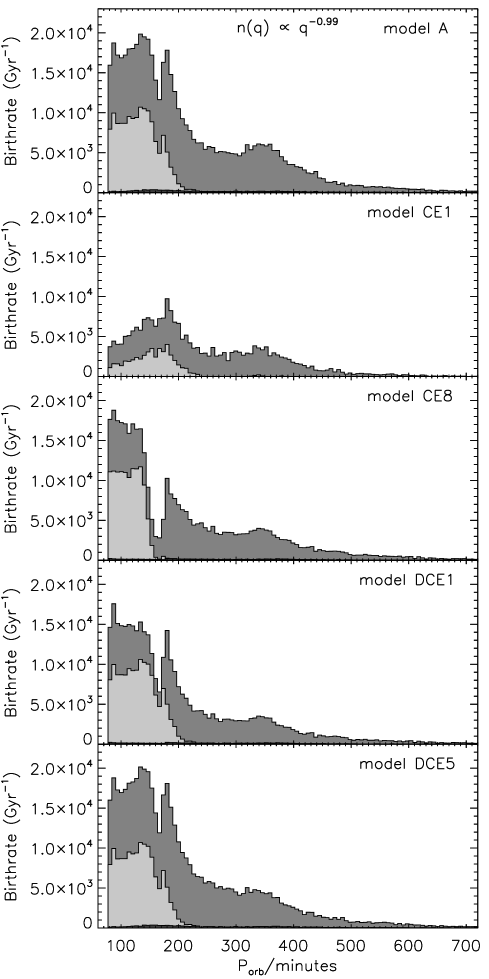
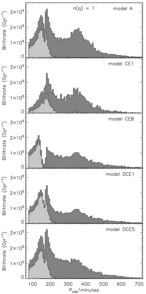
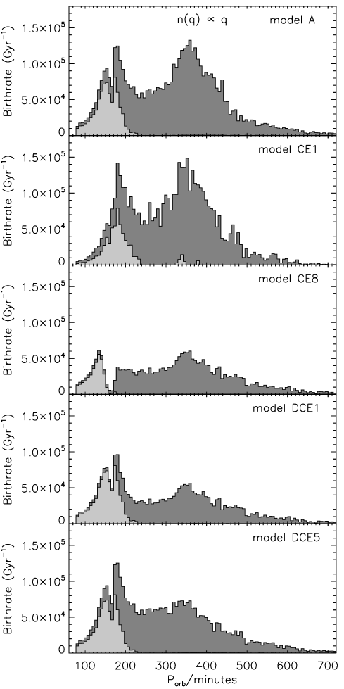
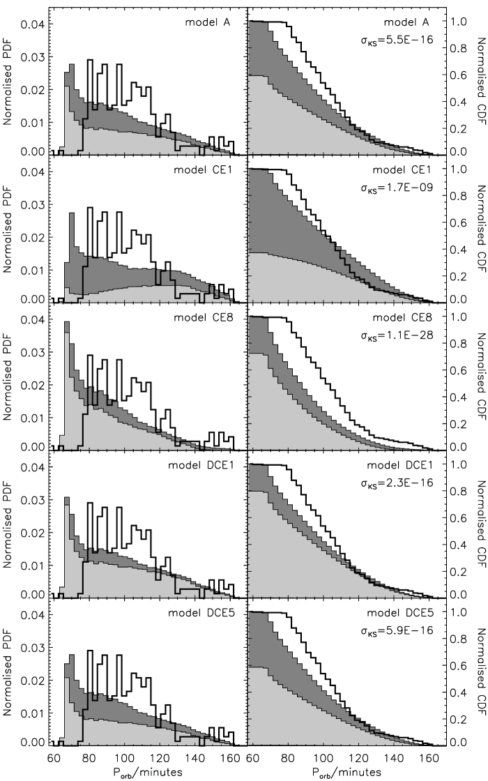
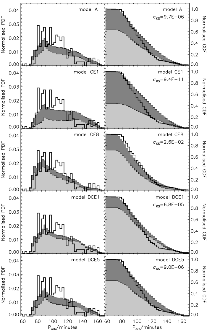
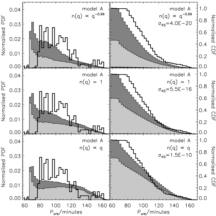

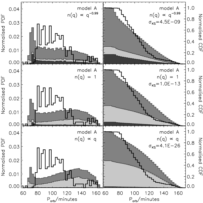
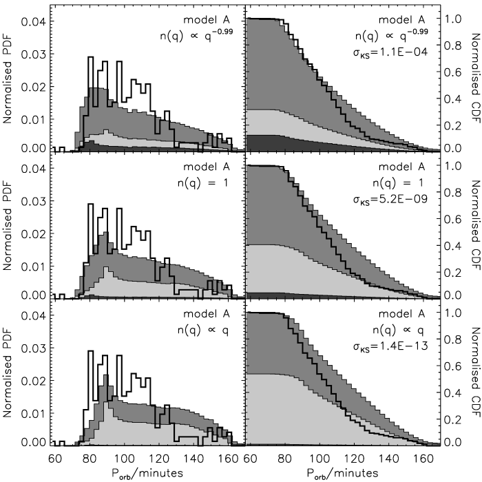
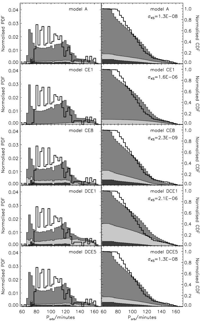
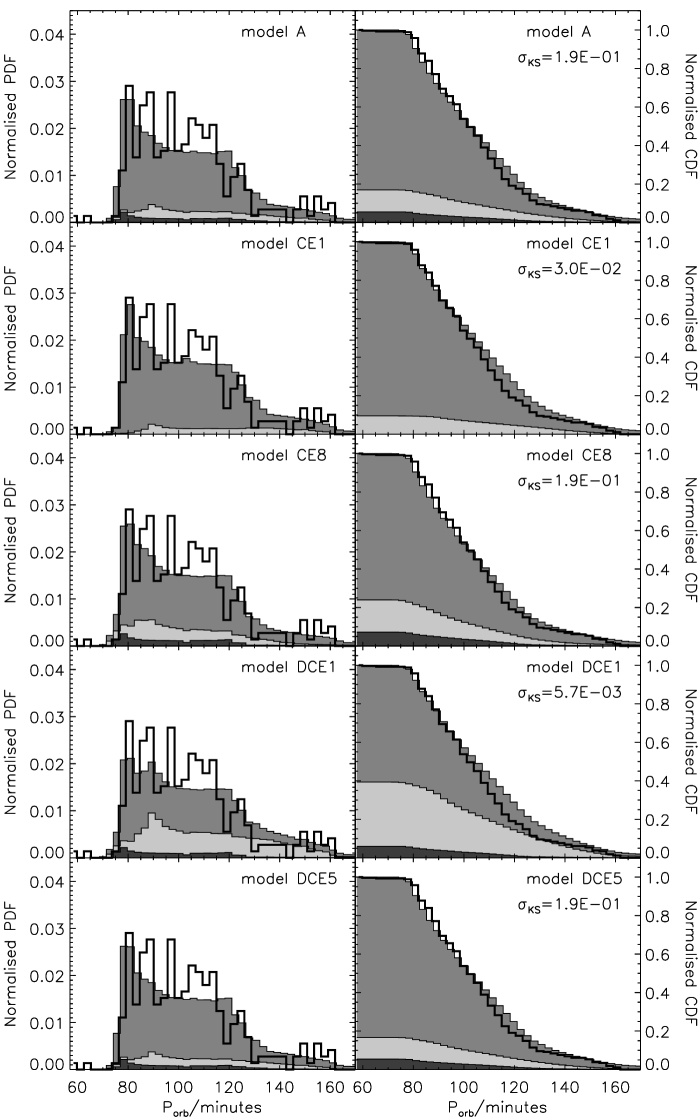
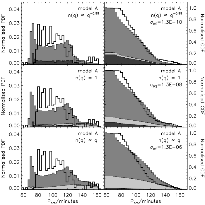
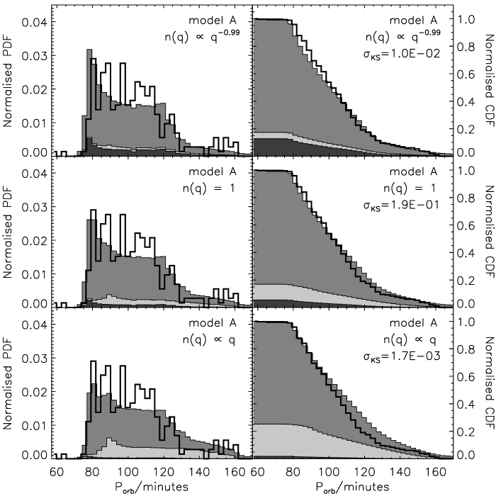

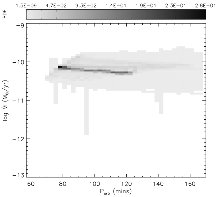
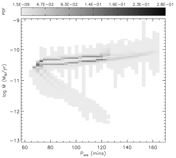
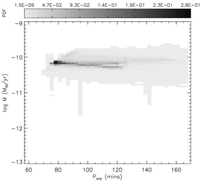
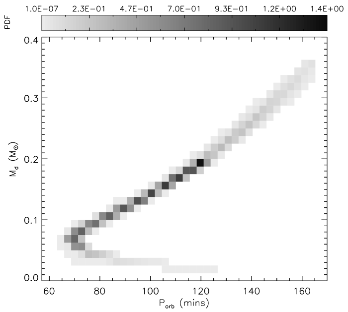
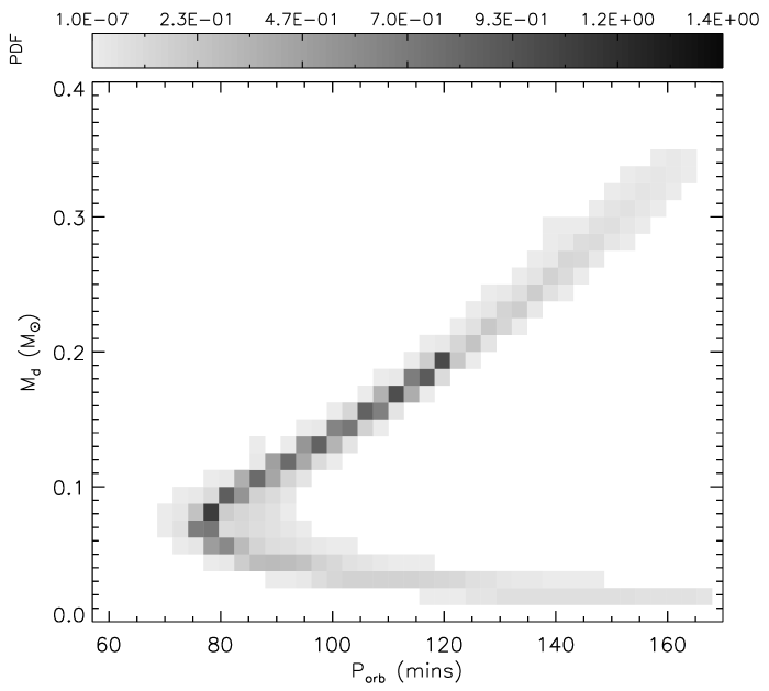
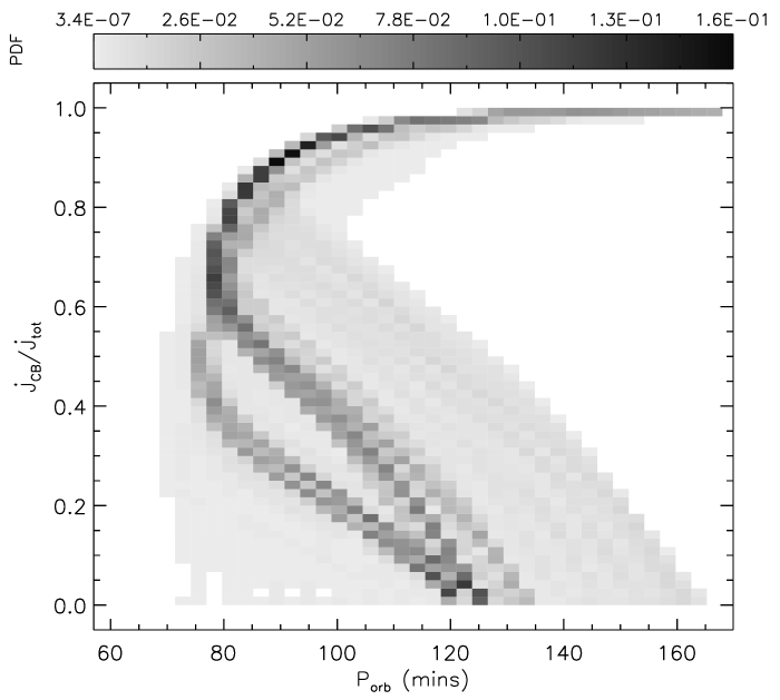
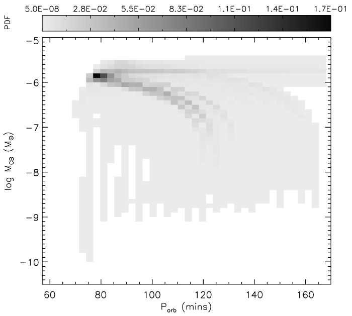
| model | |
|---|---|
| A | 0.5 |
| CE1 | 0.1 |
| CE8 | 2.5 |
| DCE1 | 0.5 for case B RLO |
| 2.5 for case C RLO | |
| DCE5 | 2.5 when |
| 0.5 when |
| model | He WD | C/O WD | O/Ne/Mg WD | Total |
|---|---|---|---|---|
| , | ||||
| A | (77.7%) | (22.2%) | (0.1%) | |
| CE1 | (54.9%) | (45.1%) | (0.0%) | |
| CE8 | (86.5%) | (13.5%) | (0.1%) | |
| DCE1 | (90.4%) | (9.6%) | (0.1%) | |
| DCE5 | (77.5%) | (22.4%) | (0.1%) | |
| , | ||||
| A | (65.8%) | (33.9%) | (0.4%) | |
| CE1 | (46.6%) | (53.4%) | (0.0%) | |
| CE8 | (76.8%) | (23.0%) | (0.3%) | |
| DCE1 | (80.0%) | (19.7%) | (0.2%) | |
| DCE5 | (65.3%) | (34.3%) | (0.4%) | |
| , | ||||
| A | (50.2%) | (48.4%) | (1.4%) | |
| CE1 | (38.6%) | (61.4%) | (0.0%) | |
| CE8 | (62.4%) | (36.6%) | (1.1%) | |
| DCE1 | (63.0%) | (35.9%) | (1.1%) | |
| DCE5 | (49.6%) | (49.0%) | (1.4%) | |
| from same IMF as | ||||
| A | (49.9%) | (48.7%) | (1.3%) | |
| CE1 | (38.1%) | (61.9%) | (0.0%) | |
| CE8 | (62.1%) | (36.8%) | (1.1%) | |
| DCE1 | (62.0%) | (36.9%) | (1.1%) | |
| DCE5 | (49.4%) | (49.3%) | (1.3%) | |
| Without CB disk | With CB disk | ||||||||
|---|---|---|---|---|---|---|---|---|---|
| model | He WD | C/O WD | O/Ne/Mg WD | Total | He WD | C/O WD | O/Ne/Mg WD | Total | |
| , | |||||||||
| A | |||||||||
| CE1 | |||||||||
| CE8 | |||||||||
| DCE1 | |||||||||
| DCE5 | |||||||||
| , | |||||||||
| A | |||||||||
| CE1 | |||||||||
| CE8 | |||||||||
| DCE1 | |||||||||
| DCE5 | |||||||||
| , | |||||||||
| A | |||||||||
| CE1 | |||||||||
| CE8 | |||||||||
| DCE1 | |||||||||
| DCE5 | |||||||||
| from same IMF as | |||||||||
| A | |||||||||
| CE1 | |||||||||
| CE8 | |||||||||
| DCE1 | |||||||||
| DCE5 | |||||||||
| Without CB disk | With CB disk | ||||||||
|---|---|---|---|---|---|---|---|---|---|
| model | He WD | C/O WD | O/Ne/Mg WD | Total | He WD | C/O WD | O/Ne/Mg WD | Total | |
| , | |||||||||
| A | 61.1/9.0 | 19.3/10.6 | 0.1/0.1 | 80.4/19.7 | 59.5/13.5 | 21.1/5.8 | 0.1/0.1 | 80.7/19.3 | |
| CE1 | 44.8/0.7 | 40.9/13.5 | 0.0/0.0 | 85.7/14.2 | 45.1/6.5 | 38.6/9.8 | 0.0/0.0 | 83.7/16.3 | |
| CE8 | 62.2/19.6 | 11.7/6.4 | 0.1/0.1 | 73.9/26.1 | 59.7/19.8 | 15.6/4.8 | 0.1/0.1 | 75.4/24.6 | |
| DCE1 | 78.4/11.6 | 6.5/3.6 | 0.1/0.1 | 84.9/15.2 | 73.1/16.6 | 7.9/2.5 | 0.1/0.1 | 81.0/19.1 | |
| DCE5 | 60.7/8.9 | 19.6/10.7 | 0.1/0.1 | 80.3/19.7 | 59.3/13.5 | 21.3/5.9 | 0.1/0.1 | 80.7/19.4 | |
| , | |||||||||
| A | 47.8/11.3 | 22.7/17.8 | 0.2/0.3 | 70.7/29.4 | 48.9/13.9 | 27.3/9.7 | 0.2/0.1 | 76.4/23.7 | |
| CE1 | 36.1/1.1 | 43.3/19.5 | 0.0/0.0 | 79.4/20.6 | 37.2/6.5 | 43.2/13.1 | 0.0/0.0 | 80.4/19.6 | |
| CE8 | 50.9/21.8 | 14.7/12.4 | 0.1/0.2 | 65.7/34.4 | 51.1/20.2 | 20.2/8.2 | 0.2/0.1 | 71.5/28.5 | |
| DCE1 | 64.7/15.2 | 10.5/9.2 | 0.1/0.2 | 75.3/24.6 | 62.8/17.8 | 13.5/5.7 | 0.1/0.1 | 76.4/23.6 | |
| DCE5 | 47.3/11.2 | 23.0/18.1 | 0.2/0.3 | 70.5/29.6 | 48.4/13.7 | 27.7/9.8 | 0.2/0.1 | 76.3/23.6 | |
| , | |||||||||
| A | 32.9/12.2 | 24.5/29.0 | 0.4/1.1 | 57.8/42.3 | 36.1/13.2 | 33.3/16.2 | 0.7/0.4 | 70.1/29.8 | |
| CE1 | 27.7/1.5 | 43.7/27.1 | 0.0/0.0 | 71.4/28.6 | 29.4/6.3 | 46.6/17.6 | 0.0/0.0 | 76.0/23.9 | |
| CE8 | 37.6/21.8 | 17.7/22.0 | 0.2/0.7 | 55.5/44.5 | 40.2/19.3 | 25.5/14.1 | 0.5/0.5 | 66.2/33.9 | |
| DCE1 | 46.2/17.2 | 15.5/20.3 | 0.2/0.7 | 61.9/38.2 | 48.0/17.7 | 21.2/12.3 | 0.5/0.4 | 69.7/30.4 | |
| DCE5 | 32.3/11.9 | 24.9/29.5 | 0.4/1.1 | 57.6/42.5 | 35.5/13.1 | 33.9/16.4 | 0.7/0.4 | 70.1/29.9 | |
| from same IMF as | |||||||||
| A | 31.7/13.3 | 23.0/30.5 | 0.4/1.1 | 55.1/44.9 | 35.4/14.1 | 32.1/17.3 | 0.7/0.5 | 68.2/31.9 | |
| CE1 | 26.9/1.7 | 42.3/29.1 | 0.0/0.0 | 69.2/30.8 | 28.7/6.7 | 45.8/18.9 | 0.0/0.0 | 74.5/25.6 | |
| CE8 | 36.4/23.2 | 16.3/22.9 | 0.2/0.8 | 52.9/46.9 | 39.8/20.3 | 24.2/14.7 | 0.5/0.5 | 64.5/35.5 | |
| DCE1 | 43.9/18.5 | 14.8/21.9 | 0.2/0.8 | 58.9/41.2 | 46.5/18.5 | 20.8/13.3 | 0.5/0.4 | 67.8/32.2 | |
| DCE5 | 31.1/13.0 | 23.4/31.0 | 0.4/1.1 | 54.9/45.1 | 34.9/13.9 | 32.6/17.4 | 0.7/0.5 | 68.2/31.8 | |