Spectral Decomposition of Broad-Line AGNs and Host Galaxies

Abstract

Using an eigenspectrum decomposition technique, we separate the host galaxy from the broad line active galactic nucleus (AGN) in a set of $4666$ spectra from the Sloan Digital Sky Survey (SDSS), from redshifts near zero up to about $0.75$. The decomposition technique uses separate sets of galaxy and quasar eigenspectra to efficiently and reliably separate the AGN and host spectroscopic components. The technique accurately reproduces the host galaxy spectrum, its contributing fraction, and its classification. We show how the accuracy of the decomposition depends upon $S/N$, host galaxy fraction, and the galaxy class. Based on the eigencoefficients, the sample of SDSS broad-line AGN host galaxies spans a wide range of spectral types, but the distribution differs significantly from inactive galaxies. In particular, post-starburst activity appears to be much more common among AGN host galaxies. The luminosities of the hosts are much higher than expected for normal early-type galaxies, and their colors become increasingly bluer than early-type galaxies with increasing host luminosity. Most of the AGNs with detected hosts are emitting at between $1\%$ and $10\%$ of their estimated Eddington luminosities, but the sensitivity of the technique usually does not extend to the Eddington limit. There are mild correlations among the AGN and host galaxy eigencoefficients, possibly indicating a link between recent star formation and the onset of AGN activity. The catalog of spectral reconstruction parameters is available as an electronic table.

1. Introduction

Quasars, and active galactic nuclei (AGNs) in general, are known to exist at the centers of galaxies, and it is believed that accretion of galactic material onto a supermassive black hole is the primary mechanism of their energy generation (e.g. Lynden-Bell, 1969; Rees, 1984). Numerous studies now suggest a close link between the growth of supermassive black holes and normal galaxies, in particular a correlation between black hole mass and galactic stellar bulge mass (e.g. Ferrarese, 2002, for a review). An understanding of the physical connection between the AGN central engine and host galaxy requires a description of the properties of both the AGN and host separately, and in relation to one another, across a wide range of intrinsic properties. However, it is observationally difficult to study the properties of both an AGN and its host galaxy. At high AGN luminosities ($M_{B}\lesssim-23$, traditionally defined as the quasar regime), the contrast between the AGN and host galaxy is so great that the host cannot be easily discerned from the AGN. At low AGN luminosities, the AGN cannot be observed without significant contamination from the host unless very high spatial resolution techniques are employed.

Much effort has been applied to the development of techniques for the spatial image decomposition of AGNs and host galaxies (e.g. Kuhlbrodt et al., 2004; McLure et al., 2000; Wadadekar et al., 1999). The results from image decomposition studies generally show that AGNs are usually found in bulge-dominated galaxies at the bright end of the luminosity function (e.g. Smith et al., 1986; Dunlop et al., 2003; Falomo et al., 2004; Floyd et al., 2004); this is especially true for radio loud AGNs and AGNs with higher luminosities (e.g. Hamilton et al., 2002; Dunlop et al., 2003). Multi-band image studies also show that the stellar populations of the host galaxies tend to be bluer, and therefore are likely to be younger, than inactive galaxies with the same morphological and luminosity characteristics (Hutchings et al., 2002; Sánchez et al., 2004; Jahnke et al., 2004a). There is also evidence for mergers or other interactions in some of the host galaxy images (Hutchings, 1987; Bahcall et al., 1997; Malkan et al., 1998; Márquez et al., 2001; McLeod & McLeod, 2001; Sánchez & González-Serrano, 2003; Sánchez et al., 2004), although it is not clear that host galaxies are more likely to be interacting than their inactive counterparts (Schade et al., 2000; Dunlop et al., 2003).

Spectroscopic studies of AGN host galaxies have usually been confined to the outer parts of the galaxies, well away from the contaminating nuclear regions (Boroson et al., 1982; Balick & Heckman, 1983; Boroson & Oke, 1984; Boroson et al., 1985; Hutchings & Crampton, 1990; Nolan et al., 2001; Miller & Sheinis, 2003). Some integrated-field spectroscopy and other spectroscopic AGN removal techniques have also been performed on a small number of AGN host galaxies (Courbin et al., 2002; Jahnke et al., 2004b). These studies have revealed both old (Nolan et al., 2001) and young (Hutchings & Crampton, 1990) stellar populations. Results supporting the interpretation of host galaxies as massive bulge-dominated systems with relatively young stellar populations were found by Kauffmann et al. (2003), who analyzed the nuclear spectroscopic properties of over $20,000$ narrow-line (type 2) AGNs found in the Sloan Digital Sky Survey (SDSS York et al., 2000). They found that nearly all type 2 AGNs reside in massive galaxies with “early-type” structural properties, but that the age, starburst fraction, and ionization state of the AGN depends on the [O iii] emission luminosity. Because type 2 AGN spectra contain little or no continuum component, Kauffmann et al. (2003) were able to separate cleanly the stellar from emission line contributions to the spectra using pure stellar galaxy templates (they did not need to remove the broad-line components of AGNs).

Recently, Hao et al. (2005a) and Dong et al. (2005) demonstrated that galaxy stellar and emission line spectral components can be separated in narrow-line and some broad-line AGNs by using galaxy eigenspectra and a power-law continuum for a possible AGN continuum component. The technique proved effective for isolating the emission line components (from the galaxy, a possible AGN, or both) that were then used to classify the galaxy as star forming or AGN (Hao et al., 2005a). Spectral principal component analysis (PCA) has been performed on both galaxy (Yip et al., 2004a) and quasar (Yip et al., 2004b) samples from the SDSS. These studies showed that galaxies and quasars can be classified based on only two or three eigencoefficients. At low luminosities, the quasar second eigenspectrum has a strong galactic component resembling the first galaxy eigenspectrum. These results suggest that a combination of both galaxy and quasar eigenspectra may be effective in separating the components of composite AGN/galaxy spectra.

In this paper we describe such a technique, and show that the galaxy and AGN components can be reliably disentangled over a wide range of galaxy types and galaxy to AGN flux fractions, even in spectra with modest signal-to-noise ratios. The technique has already been applied to a small sample of SDSS AGNs by Strateva et al. (2005), who used it to estimate AGN continuum luminosities free of host galaxy components. Here we apply the technique to over $11,000$ AGN spectra from the SDSS third data release (DR3, Abazajian et al., 2005). The properties of the AGNs and host galaxies can be studied separately or in relation to each other. In addition, the large sample size makes it possible to examine population statistics of broad-line AGNs and host galaxies in ways not possible previously.

The focus of this paper is on broad-line (“type 1”) objects, which we will generically refer to as AGNs, regardless of luminosity. Quasars are defined as broad-line AGNs with luminosities brighter than $M_{i}=-22.0$ (following the definition given in the SDSS quasar catalog by Schneider et al., 2005).

The SDSS AGN survey and dataset are described in § 2. The eigenspectrum spectral decomposition technique is described along with the results of simulation tests in § 3. The application of the technique to the SDSS AGN spectra is described in § 4, and some characteristics of the AGN and host populations are described in § 5. The results are discussed and summarized in § 6. Throughout the paper we assume a flat, $\Lambda$-dominated cosmology with parameter values $\Omega_{m}=0.3,\Omega_{\Lambda}=0.7$ and $H_{0}=70{\rm\,km\,s^{-1}Mpc^{-1}}$.

2. The SDSS AGN Sample

2.1. The Main SDSS Quasar Survey

The broad-line AGNs used for this study were selected from the SDSS. The SDSS is a project to image of order $10^{4}\,{\rm deg}^{2}$ of sky, mainly in the northern Galactic cap, in five broad photometric bands ($u,g,r,i,z$, (Fukugita et al., 1996)) to a depth of $r\sim 23$, and to obtain spectra of $10^{6}$ galaxies and $10^{5}$ quasars selected from the imaging survey. Imaging observations are made with a dedicated 2.5m telescope at Apache Point Observatory in New Mexico, using a large mosaic CCD camera (Gunn et al., 1998) in a drift-scanning mode. Absolute astrometry for point sources is accurate to better than $100$ milliarcseconds rms per coordinate (Pier et al., 2003). Site photometricity and extinction monitoring are carried out simultaneously with a dedicated 20-inch telescope at the observing site (Hogg, Finkbeiner, Schlegel, & Gunn, 2001). An assessment of the image data quality is given by Ivezić et al. (2004).

The imaging data are reduced and calibrated using the photo software pipeline (Lupton et al., 2001). In this study we use three types of magnitudes, two derived from imaging data, and one from spectroscopic data. The first magnitude we use is the point-spread function (PSF) magnitude, which is derived from a Gaussian fit to the object and a series of aperture corrections using a spatially varying PSF model (Stoughton et al., 2002). We also use “cmodel” magnitudes (Abazajian et al., 2004), which are derived from a linear combination of de Vaucouleurs and exponential profile fits to object images. The SDSS photometric system is normalized so that the $u,g,r,i,z$ magnitudes are approximately on the AB system (Oke & Gunn 1983; Fukugita et al. 1996; Smith et al. 2002; c.f. discussion by Abazajian et al. 2004). The photometric zeropoint calibration is accurate to better than $2\%$ (root-mean-squared) in the $g$, $r$, and $i$ bands, and to better than $3\%$ in the $u$ and $z$ bands, measured by comparing the photometry of objects in scan overlap regions. Spectroscopic targets are selected by a series of algorithms (see Stoughton et al., 2002), and are grouped by three degree diameter areas or “tiles” (Blanton et al., 2003). Two fiber-fed double spectrographs can obtain 640 spectra for each tile; for the main survey each tile contains 32 sky fibers, and roughly 500 galaxies, 50 quasars, and 50 stars. The wavelength range of the SDSS spectra covers approximately $3800$Å to $9200$Å at a spectroscopic resolution of about 1800. The AGN spectra used here were corrected for Galactic extinction using the reddening map constructed by Schlegel, Finkbeiner, & Davis (1998), and the average Milky Way extinction curve described by Fitzpatrick (1999). “Spectroscopic magnitudes” are derived by convolving the calibrated spectra with the SDSS $g$, $r$, and $i$ filter transmission curves that include 1.3 airmasses of extinction.

Quasar candidates are selected from the SDSS color space and unresolved matches to sources in the FIRST radio catalog (Becker, White, & Helfand, 1995), as described by Richards et al. (2002). Quasars are also often identified because the objects were targeted for spectroscopy by non-quasar selection algorithms, such as optical matches to ROSAT sources (Stoughton et al., 2002; Anderson et al., 2003), various classes of stars (Stoughton et al., 2002), so-called serendipity objects (Stoughton et al., 2002), and galaxies (Strauss et al., 2002). The images of quasar candidates selected as likely “low-redshift” ($z\lesssim 3$) objects, are allowed to be either resolved or unresolved. The SDSS photo pipeline classifies object images as resolved or unresolved based on the difference between PSF and cmodel magnitudes (Abazajian et al., 2004) (see also discussions by Stoughton et al., 2002; Scranton et al., 2002; Strauss et al., 2002). It is important for this study that resolved objects can be quasar candidates, because a large fraction of AGN spectra for which a host component can be detected have extended image profiles (see § 4.1). The completeness of the SDSS quasar selection algorithm is close to $95\%$ up to the $i$ band limiting survey magnitude of $19.1$ (Vanden Berk et al., 2005).

2.2. Selection of SDSS AGN Spectra

The primary set of quasars was selected from the catalog compiled by Schneider et al. (2005). The catalog contains $46,420$ quasars, and comprises what is believed to be nearly all of the verified quasars in the SDSS third data release (Abazajian et al., 2005). Quasars are defined in the catalog to be those extragalactic objects with absolute PSF $i$ band magnitudes brighter than $M_{i}=-22$, and with at least one emission line having a FWHM larger than $1000{\rm\,km\,s^{-1}}$. The absolute magnitudes were calculated from the observed PSF magnitudes without any attempt to subtract possible host galaxy contributions. Near the faint luminosity limit of the catalog, it is apparent from inspection that many of the quasar spectra contain host galaxy components. The fraction of quasar spectra in the catalog with clear galaxy components decreases with increasing quasar luminosity (a point that will be quantified in § 4.1).

The limit of $M_{i}=-22$ (and most other traditional limits) for the definition of a quasar is fairly arbitrary, and broad-line AGNs are clearly present at fainter magnitudes (e.g. Ho et al., 1997). It is expected that the host galaxy fraction is larger for the fainter AGNs. For this study we have extended the catalog of Schneider et al. (2005) by simply removing the absolute magnitude criterion. The AGNs were selected from the initial search list described by Schneider et al. (2005), by inspecting all of the extragalactic objects that were rejected from the quasar catalog because they did not meet the absolute magnitude limit. All of the AGNs were still required to pass the emission line width criterion. This search resulted in a sample of 3584 low-luminosity broad-line AGNs.

We will refer to the combined sample of quasars and low-luminosity broad-line AGNs as the SDSS AGN sample. The sample contains over $50,000$ broad-line AGNs. Host galaxy components will not be detectable in the majority of the AGN spectra. At redshifts beyond $0.752$, the wavelength range of the galaxy eigenspectra covered by the SDSS spectra is too small for a reliable spectroscopic reconstruction (§ 3.5). The initial data set therefore consists only of those AGNs with $z<0.752$. Spectra were also rejected for further analysis if more than $50\%$ of their pixels inside either of two wavelength regions were flagged as potentially bad by the $\tt spectro$ pipeline (see Stoughton et al. (2002) for a list of flags). The two wavelength regions are $4160<\lambda<4210$Å, where integrated flux densities are measured (§ 3.2), and the wavelength region at which an AGN spectrum and the galaxy and quasar eigenspectra overlap, which depends upon the redshift of the AGN. After the redshift and good pixel criteria are applied, the initial data set consists of $11,647$ AGN spectra.

3. Eigenspectrum Decomposition of AGN and Host Galaxy Spectra

The technique we employ to separate the spectroscopic components of composite AGN and host galaxy spectra uses separate sets of quasar and galaxy eigenspectra in linear combination. One of the goals of eigenspectrum analysis (often also called principal component analysis, PCA, or Karhunen-Loève transformation, KL) is to reduce the complexity of a dataset (compression) by constructing a (hopefully) small set of orthogonal eigenspectra that account for the bulk of the variations within a sample of objects. Yip et al. (2004a) and Yip et al. (2004b) showed that the vast majority of the spectra of galaxies and quasars in the SDSS could be described by only a relatively small number ($\lesssim 10$) of eigenspectra. In this section we demonstrate that spectra with significant contributions from both an AGN and a host galaxy can be effectively decomposed using existing sets of quasar and galaxy eigenspectra.

3.1. The Quasar and Galaxy Eigenspectra

The eigenspectra employed here are those described and made available by Yip et al. (2004a) for the SDSS galaxy sample, and by Yip et al. (2004b) for the SDSS quasar sample. The amount of information contained in each eigenspectrum is given by the relative amplitude of its eigenvalue. The galaxy sample variance is strongly concentrated in just the first few eigenspectra, with over $98\%$ of the information contained in the first three eigenspectra (Yip et al., 2004a). The quasar information is also concentrated, but not as strongly as in the galaxy case, with $\approx 92\%$ of the sample variance accounted for by the first ten eigenspectra. Yip et al. (2004b) showed that the resulting quasar eigenspectra depend on both redshift and luminosity, which causes a reduction in the information content of the top global eigenspectra (formed from the entire sample). Eigenspectra formed from subsets of quasars separated into bins of redshift and luminosity have a much more concentrated information content; meaning that fewer of these “local” eigenspectra are required to describe a quasar within a restricted redshift and luminosity bin. It was also shown that eigenspectra from a given bin can be used to reliably reconstruct spectra in adjacent bins, allowing redshift or luminosity trends to be tracked consistently (Yip et al., 2004b).

For our application, most of the AGN/galaxy spectra will be at redshifts $z<0.5$, so we primarily use the set of quasar eigenspectra in the “ZBIN 1” low redshift bin, spanning $0.08\leq z<0.53$, defined by Yip et al. (2004b). It is also important that there is little or no host galaxy contamination in the quasar eigenspectra, so that a galaxy component is reconstructed only by galaxy (and not quasar) eigenspectra. Therefore we use eigenspectra constructed from quasars in the “C1” high luminosity bin (in the low redshift range), defined by Yip et al. (2004b), which is sufficiently luminous that there is little evidence for any host galaxy component in the top eigenspectra; this bin spans an absolute magnitude range of $-24>M_{i}\geq-26$.

Galaxy or quasar spectra can be reconstructed as linear combinations of eigenspectra

$$f^{R}_{\lambda}=\sum_{k=1}^{m}a_{k}e_{k}(\lambda),$$ (1)

where $f^{R}_{\lambda}$ is the reconstructed flux density as a function of wavelength $\lambda$, and the $a_{k}$ are the eigencoefficients of the corresponding wavelength dependent eigenspectra $e_{k}(\lambda)$. Because the information content of the eigenspectra is concentrated in the first several modes, a relatively small number of eigenspectra can be used to closely approximate a given spectrum, while at the same time suppressing much of the spectral noise, and interpolating over small gaps in the spectra (Connolly et al., 1995; Connolly & Szalay, 1999; Yip et al., 2004a).

Following Connolly et al. (1995), we define two angles, called classification angles, which are formed from the first three galaxy eigencoefficients. The first $\phi$, is the mixing angle of the first two eigencoefficients, $a_{1}$ and $a_{2}$, of a galaxy spectrum

$$\phi=\tan^{-1}(a_{2}/a_{1}).$$ (2)

The second angle $\theta$, is formed from the third eigencoefficient $a_{3}$, of a galaxy spectrum

$$\theta=\cos^{-1}(a_{3}).$$ (3)

The eigencoefficients are normalized such that

$$\sum_{k=1}^{m}a_{k}^{2}=1\,,$$ (4)

where $m$ is the total number of eigenspectra used for a reconstruction. It was shown by Connolly et al. (1995) that the spectral type of a galaxy is tightly correlated with $\phi$, while post-starburst activity can be discriminated with $\theta$ (Connolly et al., 1995; Castander et al., 2001). The ability of the spectral decomposition method to accurately recover the galaxy classification angles from spectra with a wide range of characteristics is one of the primary tests of the technique. Yip et al. (2004b) showed that the first two eigencoefficients of quasar decompositions can be used to classify quasars (although the classification angle formed from the eigencoefficients was not explicitly defined). We define the classification angles for both host galaxies and quasars/AGNs in the same way, according to equations 2–4, and denote them with the subscripts $H$ and $A$ respectively: $\phi_{H},\theta_{H},\phi_{A},{\rm\,and\,}\theta_{A}$.

To test the dependence of the spectral decomposition method on signal-to-noise ratio and host galaxy fraction, galaxy and quasar templates with known eigencoefficients were modified in controlled ways and the effect on the resulting eigencoefficients were examined. The galaxy templates we used are the six high-$S/N$ templates (labeled $a$ through $f$) constructed by Yip et al. (2004a) from objects in specific regions of the projected classification plane. These were constructed to correspond to the spectra of each normal galaxy type in the atlas of nearby galaxies compiled by Kennicutt (1992). Each of the templates was reconstructed using the first five galaxy eigenspectra to obtain the eigencoefficients. A quasar template was made for this study by selecting a representative spectrum from the C1 quasar redshift-luminosity bin, and reconstructing it using the first 10 quasar eigenspectra. The spectrum was selected to have a high $S/N$, and inspected to ensure that there was no indication of a host galaxy contribution.

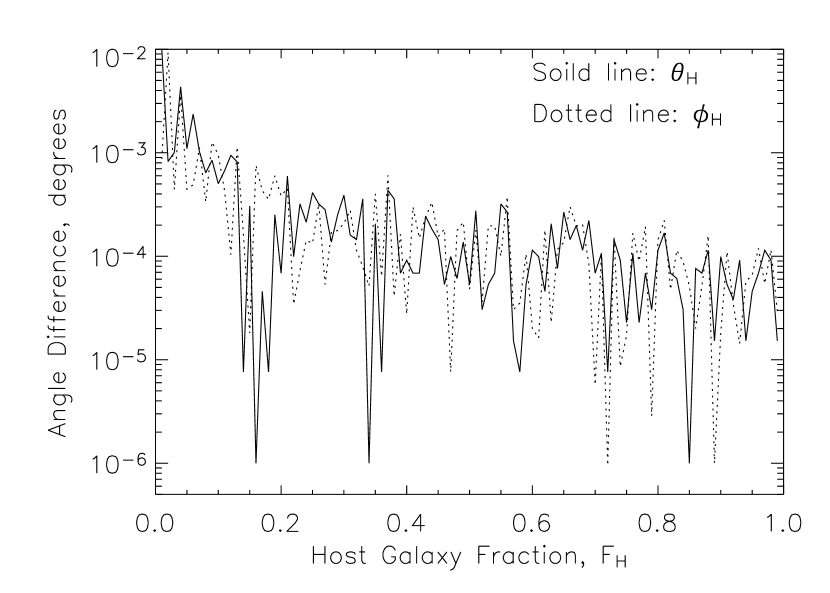
Figure 1.— The difference between the true galaxy classification angles and best-fit angles as a function of the host galaxy fraction for noiseless input spectra. The dotted line shows the $\phi_{H}$ differences, and the solid line shows the $\theta_{H}$ differences. The input spectra were constructed by combining the quasar template with the galaxy template from the $-12\arcdeg<\phi_{H}<-8\arcdeg$ range.

3.2. Recovery of Classification Angles from Noiseless Spectra

One concern about the use of two separate sets of eigenspectra is that they may not be orthogonal in combination. That is, a composite host galaxy-quasar spectrum may not be uniquely described by a linear combination of the eigenspectra from the two different bases. While Yip et al. (2004b) showed that the second global quasar eigenspectrum resembles a galaxy spectrum, it still contains quasar features (e.g. some broad emission line components), and the full galaxy component may be spread across many eigenspectra. Therefore, there is no guarantee that the quasar and galaxy components of composite spectra can be reliably reconstructed using the eigenspectrum method.

The reliability of the spectral reconstruction of composite host-quasar spectra was first tested for the ideal case of noiseless spectra. Galaxy template $d$ (from the range $-12\arcdeg<\phi_{H}<-8\arcdeg$ and $80\arcdeg<\theta_{H}<100\arcdeg$) was selected for this test because it is derived from the region with the highest density of sample galaxies. The reconstructed galaxy template was combined with the quasar template at various levels of fractional contribution. The fractional contribution of the host galaxy to the composite spectrum $F_{H}$, is defined by the integrated flux densities of the reconstructed quasar and galaxy components over the rest wavelength range $4160<\lambda<4210$Å,

$$F_{H}=\frac{\int_{4160}^{4210}{f^{R}_{\lambda,H}}\,d\lambda}{\int_{4160}^{4210}({f^{R}_{\lambda,A}}+{f^{R}_{\lambda,H}})\,d\lambda}.$$ (5)

The wavelength range was chosen because it avoids major galaxy stellar absorption lines as well as strong quasar emission lines, and it is covered by all of the SDSS spectra that can be usefully reconstructed. The noiseless spectra were fit with the combined sets of quasar and galaxy eigenspectra, using the first five galaxy and ten quasar eigenspectra, and the classification angles $\phi_{H},\theta_{H},\phi_{A}$ and $\theta_{A}$ were calculated. (It is shown in § 3.3 that three galaxy and five quasar eigenspectra are sufficient for the reconstruction, and using more does not change the results significantly.) Figure 1 shows the difference between the true angles and best-fit angles as a function of the host galaxy fraction for the noiseless input spectra. It is evident that there is no significant difference between the true and measured classification angles at any level of host galaxy contribution. Similar results were found for the quasar classification angles. The fitting technique reliably reconstructs the galaxy and quasar components in the ideal case of noiseless spectra.

Figure 2.— Average reduced $\chi^{2}$ values for reconstructed spectra compared to template spectra for varying numbers of quasar and galaxy eigenspectra. The value of $\chi^{2}$ ranges from $1.2$ at $N_{A}=1$ and $N_{H}=1$, to $1.0$ at $N_{A}=10$ and $N_{H}=5$. The average reduced $\chi^{2}$ value for each point on the grid was calculated from fits to 1000 simulated spectra.

3.3. The Number of Eigenspectra

The number of quasar and galaxy eigenspectra to use in the fitting process is an important issue. With too few eigenspectra, it will not be possible to reconstruct all of the significant details in a spectrum. The use of too many eigenspectra can lead to “overfitting” a spectrum, so that eigenspectra of higher orders begin to fit noise features.

The optimal number of eigenspectra will clearly depend upon the quality of a spectrum. In § 3.4 we discuss the dependence of the reconstructions on $S/N$ and host galaxy fraction. Here we examine the number of eigenspectra that should be used by fixing the $S/N$ and host fraction at values typical of the spectra in the SDSS. The same galaxy and quasar templates used in the previous section were combined at a galaxy fraction of $30\%$, and Gaussian noise was added to achieve a $S/N$ per pixel of $10$ (for SDSS spectra, this translates to a $S/N$ per resolution element of $\approx 12$). The template was fit using varying numbers of both host galaxy and quasar eigenspectra, $N_{H}$ and $N_{A}$ respectively, and the quality of each fit was measured by calculating the reduced $\chi^{2}$ value of the fit. Figure 2 shows the reduced $\chi^{2}$ values of the fits for each combination of the numbers of quasar and galaxy eigenspectra. The value of $\chi^{2}$ ranges from $1.2$ at $N_{H}=1$ and $N_{A}=1$, to 1.0 at $N_{H}=5$ and $N_{A}=10$. The $\chi^{2}$ value drops significantly with increasing numbers of eigenspectra, until about three galaxy and five quasar eigenspectra, at which point the values do not change greatly with the addition of more eigenspectra. Therefore, for the template used in this test, there is no justification for using more than three galaxy and five quasar eigenspectra. For the AGNs in our sample, we have generally used five galaxy and ten quasar eigenspectra, which are more than needed in most cases, but not too many that the spectra are overfitted (the reduced $\chi^{2}$ values do not drop significantly below unity).

The result that only a relatively small number of eigenspectra are required is not unexpected. The first three galaxy eigenspectra account for over $98\%$ of the variation in SDSS galaxy spectra (Yip et al., 2004a), and the first 5 quasar eigenspectra in the low-redshift, high luminosity bin account for $99.8\%$ of the SDSS quasar spectral variation in that bin. More subtle variations accounted for by higher orders are often not apparent in spectra unless the $S/N$ level is very high.

Figure 3.— The measured galaxy classification angles for the six noiseless templates, using $N_{H}=5$ eigenspectra (circles), and $N_{H}=10$ eigenspectra ($\times$’s). The boxes show the regions from which galaxy spectra were selected to form the templates. Labels show the general trend of galaxy type with $\phi_{H}$.

While a small number of eigenspectra is sufficient for the most common galaxy types, a larger number will be necessary for rare galaxy types, particularly those with very strong emission lines (Yip et al., 2004a). To illustrate this, Fig. 3 shows the measured classification angles for all six galaxy templates using both $N_{H}=5$ and $N_{H}=10$ galaxy eigenspectra. No noise or quasar component was added in this test. The measured classification angles are almost indistinguishable in the two cases for all five templates with $\phi_{H}>-40\arcdeg$. However there is a difference of about $30\arcdeg$ in $\phi_{H}$ and about $15\arcdeg$ in $\theta_{H}$ between the measurements for the extreme emission line galaxy template. The measurement made using the larger number of eigenspectra is clearly better in that case. Because of this, in cases with an initial $N_{H}=5$ measurement of $\phi_{H}<-40\arcdeg$, the spectra used in this study were decomposed a second time using $N_{H}=10$ host eigenspectra.

3.4. Dependence on Signal-to-Noise and Host Galaxy Fraction

The reliability of the component reconstruction clearly depends upon the $S/N$ of a spectrum and the relative contribution of each component. To quantify this dependence, we tested the routine on simulated spectra generated as described above but with varying amounts of noise and host galaxy contribution. For these tests, the quasar template was combined with the $-12\arcdeg<\phi_{H}<-8\arcdeg$ galaxy template. The galaxy template fraction $F_{H}$ was varied from near zero to near one. The spectroscopic noise level was varied to achieve a $S/N$ per pixel range between 5 and 30. Random noise was added to each composite template spectrum according to the desired $S/N$ level. The spectra were decomposed using $N_{H}=5$ and $N_{A}=10$ eigenspectra, and the classification angles were measured. This was repeated 1000 times for each composite template spectrum, and the rms dispersion of the $\phi$ and $\theta$ values were calculated for each combination of galaxy fraction and $S/N$.

Figure 4.— The rms dispersion, in degrees, on the measurement of $\phi_{H}$ (left) and $\theta_{H}$ (right) for simulated spectra with varying levels of $S/N$ and host galaxy contribution fraction. The contours are labeled by the value of the dispersion.

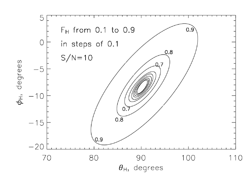
Figure 5.— Confidence contours encircling $90\%$ of the results of reconstructions to the simulated spectra, for varying values of $F_{H}$. The host galaxy fraction in the simulated spectra was varied from 0.1 to 0.9 in steps of 0.1, and the $S/N$ level was fixed to be 10. The outer three contours are labeled by the values of $F_{H}$ in the simulations. The angle $\phi_{H}$ is generally correlated with star formation rate, while $\theta_{H}$ appears to be related to post-starburst activity.

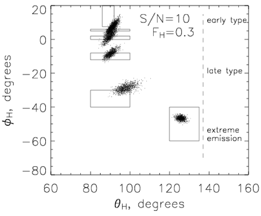
Figure 6.— The classification angles for the six host galaxy templates with 1000 simulations of added noise. The $S/N$ level of the simulated spectra was fixed at 10, and the host galaxy fraction was fixed at $F_{H}=0.3$. The boxes show the regions from which Yip et al. (2004a) selected galaxy spectra to construct the templates. Labels show the general trend of galaxy type with $\phi_{H}$.

The results for the dispersion of the $\phi_{H}$ and $\theta_{H}$ measurements are shown in Fig. 4. As expected, the dispersion decreases for increasing $S/N$ and galaxy fraction. More interesting is the fact that even at modest $S/N$ and galaxy fraction levels (say $S/N=10$ and $F_{H}=0.3$), the dispersions are only a few degrees for each angle. That is small enough to distinguish almost all of the galaxy templates from each other. Figure 5 shows the $90\%$ confidence ellipses (containing $90\%$ of 1000 random realizations) in the $\phi_{H}-\theta_{H}$ plane for a range of values of $F_{H}$, for simulations using the $-12\arcdeg<\phi_{H}<-8\arcdeg$ galaxy template, with $S/N=10$. The values of $\phi_{H}$ and $\theta_{H}$ are clearly covariant, but the confidence ellipses shrink rapidly with increasing host galaxy fraction. There are also no systematic offsets in the values of the angles at any galaxy fraction. Finally, Fig. 6 shows the measured values of $\phi_{H}$ and $\theta_{H}$ for the 1000 simulations of all six templates with $S/N=10$ and $F_{H}=0.3$. (The points are not centered in the middles of the boxes because the distributions of real galaxies are not uniform across the boxes; see Yip et al. (2004b).) All of the galaxy templates can be distinguished from each other, except for the two with $\phi_{H}>5\arcdeg$.

Figure 7.— The rms dispersion, in degrees, on the measurement of $\phi_{A}$ (left) and $\theta_{A}$ (right) for simulated spectra with varying levels of $S/N$ and host galaxy contribution fraction. The contours are labeled by the value of the dispersion.

Similar results were found for the quasar reconstructions. Figure 7 shows the dispersions of the $\phi_{A}$ and $\theta_{A}$ measurements, as functions of both $S/N$ and quasar fraction. The $\phi_{A}$ and $\theta_{A}$ dispersions are roughly twice as large as the corresponding galaxy values.

3.5. Dependence on Eigenspectrum Wavelength Coverage

The eigenspectra cover the wavelength ranges spanned by the spectra used to construct them. For the eigenspectra used here, the rest frame wavelength range is effectively $3500-7000$Å. However, as redshift increases, a decreasing fraction of the eigenspectrum wavelength range can be used, because rest frame wavelengths are shifted out of the observed range. The redshift at which there is no more usable eigenspectrum wavelength coverage is clearly an upper limit on the technique; however, a practical limit is reached at lower redshifts as the reliability of the reconstructed spectra decreases with shorter wavelength coverage.

Figure 8.— The rms dispersion, in degrees, on the measurement of $\phi_{H}$ and $\theta_{H}$ for simulated spectra with varying fractions of eigenspectrum wavelength coverage. The host galaxy luminosity fraction and $S/N$ ratio were held constant, and noise was added to the template spectra according to the $S/N$ level.

Figure 8 shows the rms dispersion of the galaxy classification angles measured for a large number of simulated spectra, as a function of the fraction of the total eigenspectrum wavelength covered. The host galaxy fraction and $S/N$ level were held constant in all of the simulations. As expected, the dispersions increase with shorter wavelength ranges. For our purposes, the dispersions become unacceptably large at a wavelength coverage fraction of about 0.5. At that point, the dispersions are comparable to those in cases with low $S/N$ and small galaxy fraction. In SDSS spectra, the redshift corresponding to a coverage fraction of 0.5 is $z_{limit}=0.752$, which is what we adopt as the upper limit for the sample selection.

The redshift limitation is not a limitation of the technique in general, but applies to the specific case of the eigenspectra used here. It is also restricted to the galaxy eigenspectra, since the quasar eigenspectra cover a much wider wavelength range. The limitation could be overcome by constructing galaxy eigenspectra that cover a wider wavelength range, especially at shorter wavelengths. This requires UV spectra of low-redshift galaxies, or optical spectra of galaxies at higher redshifts.

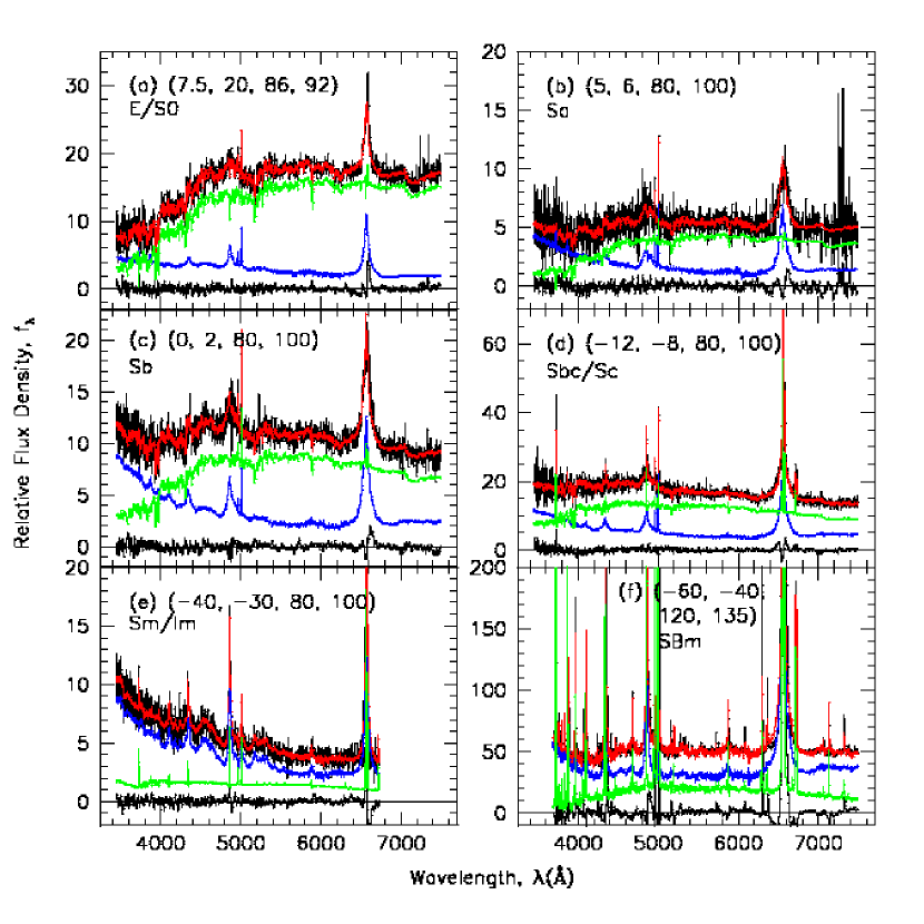
Figure 9.— Examples of eigenspectrum reconstructions of AGN/host galaxy spectra. Each panel shows the original spectrum (black), the reconstructed spectrum (red), the residual spectrum smoothed by 7 pixels (black, near $f_{\lambda}=0$), the AGN component (blue), and the host galaxy component (green). The six examples were drawn from the $\phi_{H}$ and $\theta_{H}$ regions, defined by the coordinates inside panel, from which the galaxy template spectra were constructed. The estimated morphological type of galaxies inside each region are given. The emission lines of the spectra in the lower-right panel extend well-beyond the top limit of the plot.

3.6. Example Reconstructions

Examples of fits to real spectra are shown in Fig. 9. The spectra were drawn from the SDSS dataset (see § 2), and were selected from each of the six regions for which the template galaxy spectra were created. The $S/N$ ranges from 10 to 50 and the host galaxy fractions vary from $0.25$ to $0.71$. The original spectrum, the eigenspectrum reconstruction, the residual spectrum the AGN component, and the host galaxy component are shown for each object. It is evident from the figures that the spectra are well fit by the combined eigenspectrum sets. Larger residuals occur in the regions containing strong narrow emission lines, as expected, because a larger number of eigenspectra is often required to describe narrow line features.

4. SDSS Host Galaxy and AGN Spectra

4.1. Decomposition of SDSS AGN Spectra

Figure 10.— The fraction of AGN spectra with $S/N>10$ having a detectable host galaxy, i.e. a galaxy fraction greater than $F_{H}=0.1$, as a function of absolute $i$ band cmodel magnitude, $M_{i}$. Also shown is the fraction of AGNs in the sample that have extended image morphology as a function of $M_{i}$.

The eigenspectrum decomposition method was applied to all $11,647$ AGN spectra in the initial sample. The fits to some of the spectra resulted in components that extend below zero flux density in continuum regions. Inspection of those cases showed that the AGN component dominates enough that the galaxy component is too small to be reliably estimated, that is, the galaxy fraction is usually well below $0.1$ — the practical limit discussed in § 3.4. Fits to spectra with $S/N$ ratios less than about 10 are also unreliable (§ 3.4), so those spectra are removed for further analysis. In Fig. 10 the fraction of AGNs with $S/N>10$ having a host galaxy fraction exceeding $F_{H}=0.1$ is shown as a function of the AGN absolute $i$ band magnitude. As expected, the fraction of AGNs with detectable host galaxy components drops with increasing luminosity. The detected fraction falls with luminosity in much the same way as the fraction with extended profiles in the imaging data (Fig. 10). There is a close correspondence between the classification of an AGN image as extended, and the AGN having a spectroscopic host fraction $F_{H}>0.1$. Of the AGN with $z<0.752$, $52\%$ are extended, and $61\%$ have $F_{H}>0.1$. Of the AGN with extended images, $89\%$ have $F_{H}>0.1$ compared with only $30\%$ in the AGN sample with unresolved images.

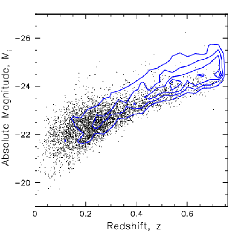
Figure 11.— The absolute $i$ band cmodel magnitude, $M_{i}$, vs. redshift for the SDSS AGN sample with $S/N>10$, up to a redshift of $z=0.752$. Dots represent AGNs for which a host galaxy was reliably detected; that is the spectra have a host galaxy fraction $F_{H}>0.1$. Contours represent the region occupied by AGNs without a reliably detected host galaxy. There are $7664$ AGNs in the $S/N>10$ sample, $4666$ of which have a detected host galaxy. The AGNs with detectable hosts are generally at lower luminosities and redshifts.

Figure 11 shows the $i$ band cmodel (total flux) absolute magnitude vs. redshift for the initial sample of $7664$ SDSS AGN with $S/N>10$; squares represent the 4666 AGNs for which there is a “reliably” detected host galaxy. At redshifts greater than about $0.4$, the hosts of less luminous AGNs are often undetected because the $S/N$ is low, and they are undetected in high luminosity AGNs because the host component fraction is too low. For most of the analysis that follows, we will omit AGNs with a host component fraction less than $F_{H}=0.1$, or a median spectroscopic $S/N$ per pixel in the $i$ band wavelength region of less than 10.

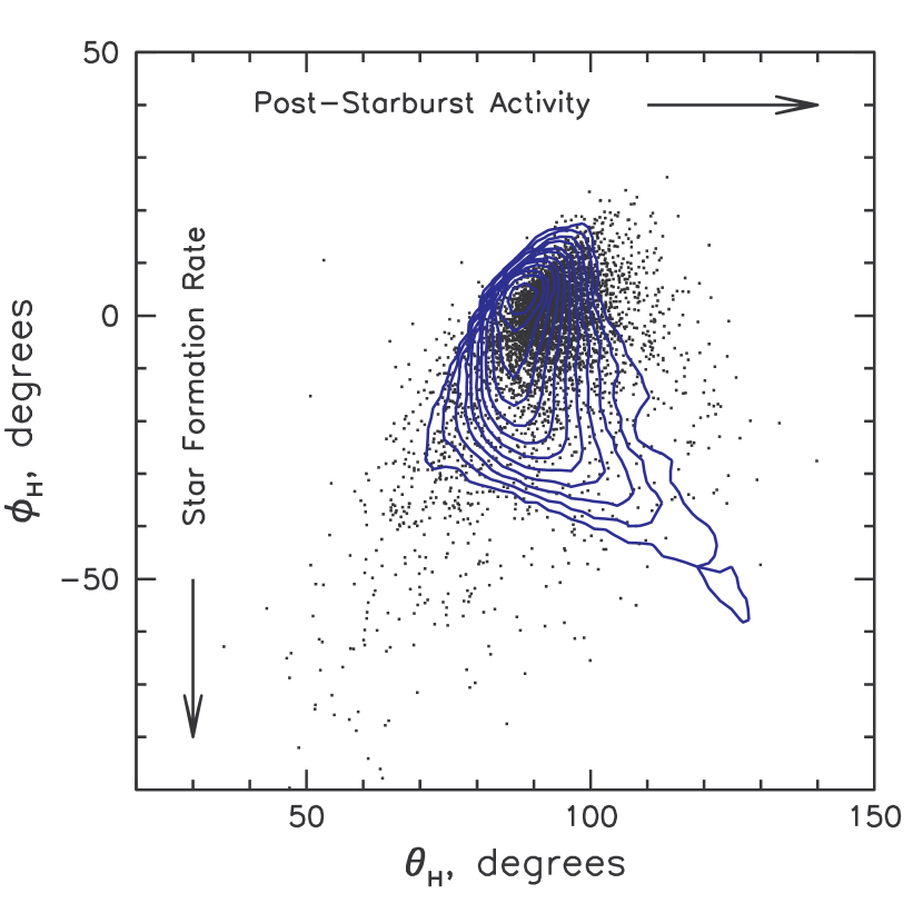
Figure 12.— The galaxy classification angles (points), $\phi_{H}$ and $\theta_{H}$, found for SDSS broad-line AGN spectra with $z<0.752$, $S/N>10$, and a host galaxy fraction $F_{H}>0.1$. There are $4666$ AGNs in the sample. The contours show the distribution of the classification angles for non-active galaxies from the sample described by Yip et al. (2004a); each contour level differs by a factor of two relative to adjacent levels. Labels show the general trends of star formation rate and post-starburst activity with the classification angles.

The galaxy classification angles for the fits to the 4666 “reliably” detected host galaxies are shown in Fig. 12. The distribution of host galaxy angles is clustered in a relatively small region, as are those of the normal galaxies analyzed by Yip et al. (2004a), which are shown with density contours in the figure. Labels show the general trends of star formation and post-starburst activity with the classification angles; however, the labels are meant only to suggest the correlations, but not that there is a strict one-to-one correspondence. A more detailed comparison of the distribution relative to normal galaxies is discussed in § 5.

Information for the objects used in this study is tabulated in an electronic table, the column description for which is given Table 1. The information is described in the electronic version of Table 2, which includes all (11,647 total) SDSS broad-line AGNs with redshifts $z<0.752$ for which an eigenspectrum reconstruction was attempted. The table includes the SDSS coordinate name, coordinates, redshift, plate number, fiber number, spectroscopic MJD, imaging morphology, spectroscopic $S/N$ in the $i$ band, magnitudes, luminosities (described in § 4.2), host galaxy fraction ($F_{H}$), and the AGN and host galaxy classification angles. Default values (set to zeros) of the reconstructed spectral parameters are given if either the quasar or host galaxy reconstructed spectra had negative flux densities in the $4160-4210$Å continuum region. The objects are listed regardless of $S/N$ or host galaxy fraction, $F_{H}$; users of the dataset can therefore apply any range of selection cuts to the sample.

4.2. Luminosity Determination

Estimates of the luminosities of the host galaxy and AGN components were made by measuring rest frame absolute magnitudes in the SDSS $g$ and $r$ passbands. Normally, absolute magnitudes are determined by measuring the apparent magnitude of an object in an observed frame passband, then applying the distance modulus (using a specific cosmology) and a K-correction, which accounts for the difference between the observed frame and rest frame flux density covered by a given passband. The wavelength range of the eigenspectra cover the SDSS $g$ and $r$ bands completely, so synthetic magnitudes can be constructed without the need for K-corrections. The selection of the SDSS $g$ and $r$ filters also allows for direct comparison between the results here and those of other SDSS galaxy studies, such as the ones by Bernardi et al. (2003c, b) and Hogg et al. (2004).

The rest frame apparent magnitudes were measured directly from the reconstructed spectra by convolving the spectra with the SDSS filter transmission curves, including 1.3 airmasses of extinction, after shifting the spectra to the rest frame and multiplying the flux densities by the redshift expansion factor, $1+z$. The distance modulus (as a function of redshift and the selected cosmology) was applied to the apparent magnitudes to determine the absolute magnitudes; K-corrections are not necessary. The absolute magnitudes of the reconstructed AGN component, the reconstructed host galaxy component, and the total spectrum of each object were determined using the spectroscopic convolution technique.

The determination of the absolute magnitudes using the spectroscopic convolution technique is possible due to the high quality of the SDSS spectrophotometry. The airmasses of the spectroscopic observations vary from plate to plate, so slight improvements could perhaps be made by adjusting the airmass of the extinction applied to the transmission curves. Additionally, small uncertainties could be introduced if fibers are not precisely centered on the active nuclei. However, a direct comparison between the stellar imaging and spectroscopic magnitudes for tens of thousands of stars in the SDSS DR3 sample, shows an rms variation of less than 0.06 magnitudes in the $g$, $r$, and $i$ bands at a spectroscopic $S/N$ of 10. That is significantly less than the uncertainty expected to be introduced by quasar variability. We expect the spectrophotometric accuracy to be somewhat lower than $0.06$ magnitudes for the AGN and host components separately, due to the uncertainties of the eigenspectrum reconstruction technique (§ 3).

Before using the magnitudes to study the properties of the objects, a correction must be applied to account for the finite angular width of the SDSS spectroscopic fibers, which subtend only a $3\arcsec$ diameter on the sky. Not all of the collected light from an active nucleus or host galaxy will be covered by a fiber, and the fraction of the total intensity entering the fibers will depend on the sizes of the images. An AGN component is spatially unresolved, while a host galaxy may be extended, so the correction factor applied to account for the finite fiber diameter will be different for each component. In addition, varying seeing conditions can affect the amount of light entering the spectroscopic fibers, even from unresolved sources.

The offsets needed to correct the (unresolved) AGN spectroscopic magnitudes were determined by comparing the spectroscopic magnitudes of non-variable early-type stars observed in the SDSS spectroscopic survey to their so-called “cmodel” magnitudes. The cmodel magnitudes $m_{c}$ (Abazajian et al., 2004), which are derived from model profile fits to the images, are designed to include nearly all of the flux of both point sources and extended galaxies. The mean observed frame magnitude offsets in the $g$, $r$, and $i$ bands were determined for each spectroscopic plate separately, to account for varying observing conditions. Each plate corresponds to observations of about 25 usable stars. The mean offsets were found by weighting each star by the square of its spectroscopic $S/N$, although the weights did not usually significantly affect the results.

In the analysis that follows, the magnitude offsets $\Delta g_{A}$ and $\Delta r_{A}$, were applied to each set of rest frame AGN absolute $g$ and $r$ magnitudes. Because the $g$, $r$, and $i$ offsets were determined in the observed frame, the rest frame $g$ and $r$ corrections applied to the AGN magnitudes were interpolated from the two closest observed frame offsets, at the redshifted central wavelengths of the $g$ and $r$ bands. Interpolation caused only minor corrections to the magnitude offsets, because the mean differences among the offsets of the three passbands are only about $0.02$ magnitudes. This is much smaller than the uncertainties between the spectroscopic and imaging epochs introduced by AGN variability, which are typically a few tenths of a magnitude (Vanden Berk et al., 2004), and become relevant when correcting the galaxy magnitudes. There are contributions to the uncertainty in the AGN magnitude corrections from photometry, the spectroscopic decomposition, and varying observing conditions. The rms dispersion of the spectroscopic to cmodel magnitudes for stars (noted above), places a lower limit on the uncertainty of $0.06$ magnitudes. We estimate the typical total uncertainty to be up to a few tenths of a magnitude. The corrected AGN absolute magnitudes $M_{g,A}$ and $M_{r,A}$, and the $\Delta g_{A}$ and $\Delta r_{A}$ values applied to the AGN spectroscopic absolute magnitudes are given in the electronic version of Table 2. Default values (set to zeros) are given for the quantities if the spectroscopic decomposition was non-physical (see § 4.1).

A significantly larger fraction of the host flux is expected to fall outside the fiber area, compared to the AGN flux. The same method used to correct the AGN flux cannot be used to correct the host galaxy component flux, because host galaxy sizes and profiles can vary greatly from object to object. Instead, we estimate the total host galaxy flux by subtracting the corrected AGN flux from the total photometric cmodel flux of the AGN plus host galaxy. In practice, the magnitude offset for a host galaxy, $\Delta m_{H}$, was found by estimating the ratio of the cmodel (subscript $c$) and spectroscopic (subscript $s$) fluxes of the host galaxy

$$\Delta m_{H} = m_{c,H}-m_{s,H}$$ (6)

$$= -2.5\log(f_{c,H}/f_{s,H})\,.$$ (7)

The host galaxy cmodel to spectroscopic flux ratio is a measure of the amount of host galaxy flux lost outside a spectroscopic fiber. The ratio cannot be measured directly, because of the contribution of the AGN component, but it can be estimated by subtracting the estimate of the AGN flux

$$\frac{f_{c,H}}{f_{s,H}} = \frac{1}{f_{s,H}}(f_{c,T}-f_{c,A})$$ (8)

$$= \frac{1}{f_{s,H}}(S_{T}f_{s,T}-S_{A}f_{s,A})$$ (9)

$$= S_{T}{F}^{-1}_{m,H}-S_{A}(F^{-1}_{m,H}-1)\,,$$ (10)

where the subscript $T$ refers to the total of the AGN (subscript $A$) and host (subscript $H$) quantities, and the cmodel to spectroscopic flux ratios are

$$S_{T} = f_{c,T}/f_{s,T}$$ (11)

$$S_{A} = f_{c,A}/f_{s,A}\,.$$ (12)

The quantity $F_{m,H}$ is the spectroscopic host contribution fraction, similar to $F_{H}$ defined by Eq. 5, but using the flux in the rest frame $g$ or $r$ bands. The result for the host galaxy magnitude correction is

$$\Delta m_{H} = -2.5\log(S_{T}F^{-1}_{m,H}-S_{A}(F^{-1}_{m,H}-1))\,.$$ (13)

The magnitude offsets were applied to the host galaxy absolute magnitudes in the analysis of the following sections. The cmodel to spectroscopic flux ratios, $S_{A}$ and $S_{T}$, can only be determined in the observed frame, so the values used in Eq. 13 were interpolated from the observed frame to the redshifted wavelengths of the $g$ and $r$ bands. While the corrected magnitudes should give an accurate estimate of the luminosities for the sample as a whole, the values for individual cases may be less reliable due to measurement uncertainties, unaccounted for differences in observing conditions, AGN variability, and inaccuracies in the spectral reconstruction. The typical uncertainty from those sources is estimated to be a few tenths of a magnitude, but larger than the uncertainty for the AGN measurements. In a small number of cases, the “corrections” make the total host luminosities fainter than the spectroscopic luminosities. The result of the uncertainties is to broaden the distribution of luminosities. In any case, the corrected host galaxy absolute magnitudes are listed in the electronic version of Table 2, along with the magnitude offsets $\Delta g_{H}$ and $\Delta r_{H}$ that were applied to the spectroscopic magnitudes, so that the results may be compared between the spectroscopic and corrected luminosities. Default values (set to zeros) are given for the quantities if the spectroscopic decomposition was non-physical (see § 4.1).

5. Results

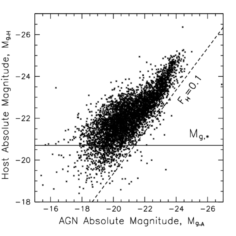
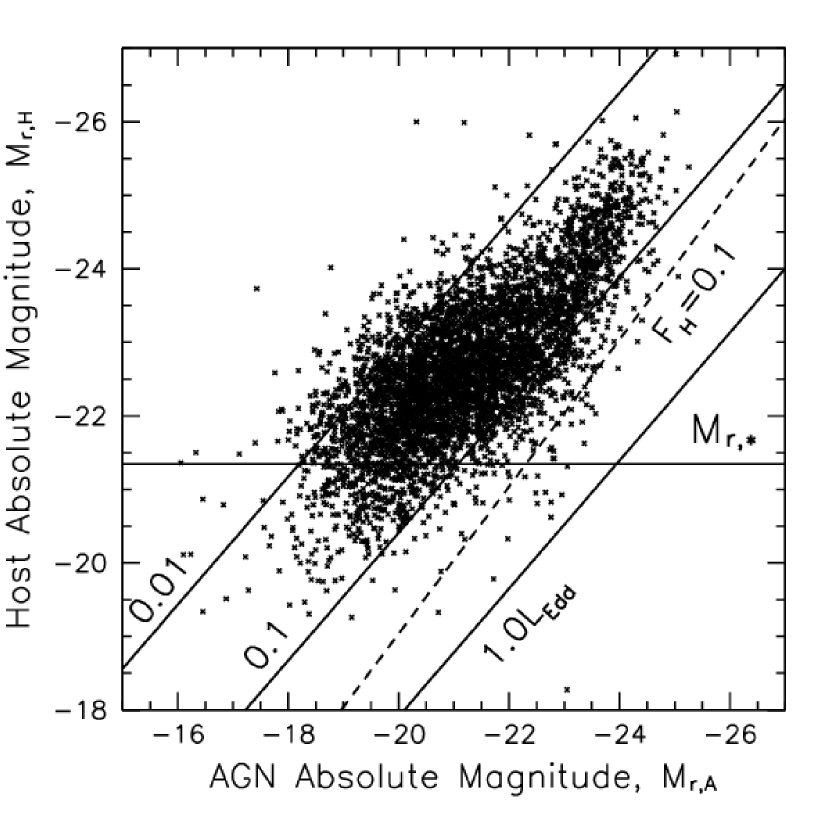
Figure 13.— Absolute $g$ band (left) and $r$ band (right) magnitudes of the AGN and host galaxy components, $M_{H}$ and $M_{A}$ respectively. The dashed diagonal lines marked $F_{H}=0.1$ correspond to a host galaxy fraction of 0.1 in each band, adjusted for the average correction from spectroscopic to cmodel magnitudes, and closely mark the sensitivity limits for the detection of host galaxies. The horizontal lines show the evolution corrected characteristic magnitude of early type galaxies without broad-line AGNs, $M_{*}$. The solid diagonal lines in the $r$ band plot show the host luminosity at which an AGN would be expected to radiate at $0.01,0.1$, and $1.0$ times the Eddington luminosity, $L_{Edd}$.

5.1. Comparison of AGN and Host Galaxy Luminosities

It was shown in § 4.1 that the fraction of AGNs with a detectable host galaxy component ($F_{H}>0.1$) decreases with AGN luminosity. Fig. 13 shows the host galaxy absolute magnitudes vs. the AGN absolute magnitudes for all of the objects with a spectroscopic $S/N>10$. The AGN and galaxy luminosities appear to be closely correlated in both the $g$ and $r$ bands. This is due in part to the increased difficulty of detecting a host galaxy as its fractional contribution to the spectra decreases. The dashed line shows where the spectroscopic host luminosity contributes $10\%$ to the total luminosity, adjusted for the average magnitude changes to the AGN and host components (§ 4.2), and corresponds closely to the galaxy fraction reliability limit, $F_{H}=0.1$ discussed in § 3.4. The selection function, that is, the fraction of spectra in which a host galaxy could be detected, decreases toward that limit. Points may extend beyond the limit (and a few do), depending upon the spectroscopic to cmodel magnitude corrections described in § 4.2. A correlation between the host and AGN luminosities cannot be established without a more careful analysis of the selection function (which we defer to future work). However, if the (unplotted) AGNs with hosts outside of the detection limits radiate at less than the Eddington limit (see below), there would be a very strong correlation between the AGN and host galaxy luminosities.

Also shown in Fig. 13 are the evolution corrected characteristic absolute magnitudes for early type galaxies (without broad emission line components), $M_{g,*}=-20.70$ and $M_{r,*}=-21.35$, as found by Bernardi et al. (2003c) for the median redshift of our sample, $\langle z\rangle=0.236$. The median values of the host absolute magnitudes are $\langle M_{g,H}\rangle=-22.03$ and $\langle M_{r,H}\rangle=-22.62$, which are clearly more luminous than typical elliptical galaxies. There is also a wide distribution in the host luminosities at every AGN luminosity.

A number of image decomposition studies have found that there is a lower threshold to the galaxy luminosity for a given AGN luminosity. This host–AGN luminosity threshold is thought to arise from scaling relationships among bulge luminosity, bulge mass, black hole mass, and Eddington luminosity. For example, Dunlop et al. (2003) found that quasars are typically radiating at $1$–$10\%$ of their Eddington luminosities, which in effect establishes a scaling relation between AGN luminosity and black hole mass. As there is also a correlation between black hole mass and bulge mass and luminosity, one expects to find a scaling relation between AGN and host galaxy luminosity. Thus, a given AGN luminosity requires a host galaxy that is sufficiently massive and luminous to harbor a black hole of the mass inferred from the Eddington ratio.

We have plotted the expected relationships between AGN and host luminosities for the $r$ band in Fig. 13, for Eddington luminosity ratios $L_{A}/L_{Edd}=1.0,0.1$, and $0.01$. The relationship between galaxy luminosity and black hole mass was estimated by assuming the $r$ band bulge mass-to-light ratio found by Bernardi et al. (2003c), a black hole mass to bulge mass of $0.0012$ (e.g. McLure & Dunlop, 2002), and assuming that the host luminosity is due entirely to a bulge component. The relationship between black hole mass and AGN luminosity was estimated by assuming a $10\%$ accretion radiation efficiency for the bolometric Eddington luminosity, and using the $V$ band to bolometric correction factor given by Elvis et al. (1994) (which should be close to the $r$ band factor within the uncertainties). Equating the black hole masses inferred from the galaxy luminosity and AGN luminosity gives the relationship between the two luminosities as a function of the Eddington ratio. For most spectra, the sensitivity limits of our study do not extend to an Eddington ratio of unity, but only to $L_{A}/L_{Edd}$ of a few tenths. The vast majority of our AGNs appear to be radiating at greater than $0.01L_{Edd}$. It is possible that the sample is missing low-luminosity AGNs with broad emission lines that are too weak to be detected in the SDSS spectra. Those objects could have $L_{A}/L_{Edd}$ much smaller than $0.01$, and therefore could populate the upper left regions of the plots in Fig. 13. Until such objects can be confirmed or ruled out, we cannot conclude that there is a lower limit to $L_{A}/L_{Edd}$.

Because we have spectroscopic information for the AGN components, it will be possible in many cases to derive estimates for the black hole masses based on the AGN broad emission line widths and the relationship between broad emission line region size and luminosity; we leave these issues to be addressed in future work. In any case, we can conclude that AGNs may reside in hosts with a wide range of luminosities, but that in general the hosts of AGNs with $M\lesssim-18$ are significantly more luminous than galaxies without strong broad line AGNs.

5.2. Host Galaxy Colors

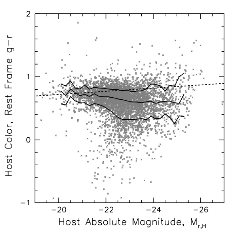
Figure 14.— Rest frame host galaxy color vs. host galaxy absolute magnitude in the $r$ band, $M_{r,H}$. The median value of the color in bins of 0.2 magnitudes is shown along with the $68.3\%$ confidence limits. The dashed line shows the color-absolute magnitude relation for early type galaxies found by Bernardi et al. (2003c).

The host galaxy rest frame ($g-r$) color is shown as a function of host absolute magnitude, $M_{r,H}$, in Fig. 14. For clarity, the mean colors and $68.3\%$ confidence envelope in bins 0.2 magnitudes wide are also shown, connected by lines. There appears to be a negative correlation of host color with luminosity, such that the hosts become bluer at higher luminosities. There is also a fairly wide distribution of colors at any given luminosity. Aside from measurement uncertainties, it is possible that the the wide distribution of colors and the luminosity trend are due to a wide distribution of galaxy types that changes with luminosity, because the colors of galaxies differ by type (cf. Hogg et al., 2004). The straight line in Fig. 14 shows the color-luminosity relation for elliptical galaxies found by Bernardi et al. (2003a), which is similar to the relation for bulge-dominated galaxies found by Hogg et al. (2004). The range of host galaxy colors is much wider than the dispersion around the elliptical color-luminosity relation, which is less than $0.1$ magnitude (Bernardi et al., 2003a). The color line for elliptical galaxies describes the host galaxy colors reasonably well at low luminosities ($M_{r,H}>-21.5$), but it becomes increasingly redder than the majority of the hosts at high luminosity. This implies that if host galaxies are mainly ellipticals or otherwise bulge-dominated, for a given luminosity they are bluer than the same types of galaxies that do not contain an observed AGN. The results may instead mean that the types of galaxies that contain AGNs change with luminosity, such that disk-dominated hosts become more common at higher luminosity. However, not only do most image decomposition studies find that the majority of host galaxies are bulge-dominated, but it also appears that bulge-dominated hosts are more common at higher luminosities (Dunlop et al., 2003). Multi-band photometric imaging studies also support the idea that the host galaxies are bluer than their non-active counterparts (Hutchings et al., 2002; Sánchez et al., 2004; Jahnke et al., 2004a).

Bernardi et al. (2003a) showed that the color luminosity relation for early type galaxies is a consequence of a strong dependence of color on stellar velocity dispersion. Based on this, we would expect the redder hosts in our sample at a given luminosity to have a higher velocity dispersion, and consequently a larger black hole mass. However, if the star formation rate is related to the presence of an AGN, that prediction may not hold. There is evidence from the eigencoefficients, described in § 5.3, that the hosts are dominated by post-starburst galaxies, which would likely change both the color-velocity dispersion and color-luminosity relation from those of non-active ellipticals. Further analysis in the future of the spectroscopic components to estimate velocity dispersion and black hole mass should help shed light on these issues.

The nuclear colors of an AGN are expected to change through time in a number of possible evolutionary sequences. For example Storchi-Bergmann et al. (2001) describe a scenario in which a merger event would both fuel AGN activity, and trigger circumnuclear star formation early in the process. Dust associated with the star formation may reprocess the nuclear light, making it appear red, so that in this early phase the galaxy would be classified as an ultraluminous infrared galaxy (e.g. Cid Fernandes et al., 2001; Bushouse et al., 2002). With time, dust is removed and the starburst fades, so that an unobscured AGN combined with an older stellar population dominate the nucleus. The objects in our study may be in such a later evolutionary phase, as long as the aged nuclear stellar population is younger than it would have been in the absence of the triggering event.

5.3. Host Galaxy Spectroscopic Classification

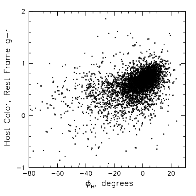
Figure 15.— Host galaxy rest frame $g-r$ color vs. $\phi_{H}$ angle values for spectra with $S/N>10$ and $F_{H}>0.1$.

Further information about the classification of the host galaxies and the AGNs is contained in the eigencoefficients. The relative strengths of the eigencoefficients contain information about the physical properties of the galaxy and AGN components. While there has yet been no quantitative calibration of the eigenspectra with physical parameters, there are clear qualitative correlations. The first few AGN eigenspectra are related to the so-called “eigenvectors 1 and 2” in observed parameter space as defined by Boroson & Green (1992), and it is believed that the eigenvectors are indicators of black hole mass and accretion rate (Boroson, 2002). The galaxy classification angles, $\phi_{H}$ and $\theta_{H}$, are related to star formation rate and the presence of post-starburst activity respectively (Yip et al., 2004a; Connolly et al., 1995; Castander et al., 2001). Figure 15 shows how the $g-r$ host galaxy colors, discussed in §§ 5.1 & 5.2, are related to the first galaxy classification angle, $\phi_{H}$. The angle $\phi_{H}$ and the host color are correlated, as expected given the qualitative relation between $\phi_{H}$ and star formation rates.

Figure 16.— Distribution of the host galaxy $\phi_{H}$ angle values for spectra with $S/N>10$ and $F_{H}>0.1$ (solid histogram). The dashed histogram shows the $\phi_{H}$ distribution for normal galaxies, found by Yip et al. (2004a).

Fig. 16 shows the distribution of $\phi_{H}$ for all of the reliably detected host galaxies with $F_{H}>0.1$ and spectroscopic $S/N>10$. Also shown is the $\phi_{H}$ distribution for the normal galaxies analyzed by Yip et al. (2004a). There are clear differences in the distributions. The host galaxy distribution is shifted to slightly more negative (bluer color) values, and there is a much less pronounced (and blueward shifted) narrow peak at $\phi_{H}\approx 5\arcdeg$ compared to the inactive galaxies. The distribution of the host $\phi_{H}$ values probably indicates that the host star formation rates are generally higher than for galaxies without AGNs. That would be true especially if the morphology distribution of the hosts relative to other galaxies is weighted toward ellipticals, as indicated in a number of imaging studies (e.g. Jahnke et al., 2004a; Sánchez et al., 2004; Hamilton et al., 2002; Percival et al., 2001; Schade et al., 2000).

Figure 17.— Distribution of the host galaxy $\theta_{H}$ angle values for spectra with $S/N>10$ and $F_{H}>0.1$ (solid histogram). The dashed histogram shows the $\phi_{H}$ distribution for normal galaxies, found by Yip et al. (2004a).

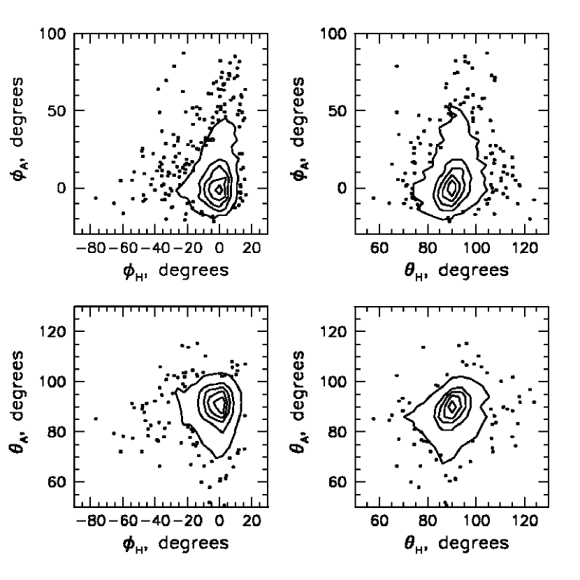
Figure 18.— The relationships among the AGN and host galaxy classification angles. Contours are spaced by density differences of approximately $20\%$ of the peak value. Points are shown if they fall, or nearly fall, outside of the lowest density contour. There are mild but significant correlations among the classification angles, except for $\theta_{A}$ vs. $\phi_{H}$.

There is a much more dramatic difference in the distributions of the second galaxy classification angle, $\theta_{H}$, shown in Fig. 17. The inactive galaxy distribution is strongly peaked at $\theta_{H}\approx 89\arcdeg$, while the host galaxy distribution is not only shifted to higher angles (a peak at $\theta_{H}\approx 93\arcdeg$), but is much wider, and extends to angles at which there are virtually no inactive galaxies. A possible interpretation is that the population of AGN hosts contains a relatively large fraction of post-starburst galaxies. Post-starburst (also called E+A) galaxies are characterized by Balmer jumps and high-order Balmer absorption lines, indicative of stellar populations of order 100 Myr old, but with little or no narrow emission lines that would imply current star formation (Dressler & Gunn, 1983). The third galaxy eigenspectrum has properties similar to those of post-starburst galaxies (Yip et al., 2004a): a blue continuum and strong Balmer absorption features, implying a relatively young stellar population, but also features anticorrelated with the continuum which reduce the narrow emission lines, and therefore indicate suppressed star formation. Post-starburst activity may therefore be indicated by $\theta_{H}$ which is a measure of the relative strength of the third galaxy eigenspectrum. A strong third eigenspectrum does not mean that there is no current star formation in a galaxy, nor that the host galaxy can be classified as a post-starburst, only that there is a component of the galaxy spectrum that resembles a post-starburst galaxy.

Spectacular examples of post-starburst AGNs (broad-line AGNs associated with a post-starburst host) have been studied in some detail (Brotherton et al., 1999; Canalizo et al., 2000; Brotherton et al., 2002). In a study of so-called “transition” AGNs — objects with characteristics of both AGNs and ultra-luminous infrared galaxies — Canalizo & Stockton (2001) found nearly all of the host galaxies had post-starburst spectra. Post-starburst AGNs virtually always show morphological evidence for recent mergers or other interactions; however, the evolutionary stages of the AGNs and the relation to the post-starburst activity is not clear. If $\theta_{H}$ is an indicator of post-starburst activity which is somehow linked to triggering AGNs, the link may be reflected in a relation between $\theta_{H}$ and black hole mass, as the black holes in young AGNs would be expected to be less massive than in older AGNs for a given accretion rate.

Assuming the eigenspectra are physically meaningful, connections among the AGN and host components may be evident in the eigencoefficients. The AGN and host galaxy classification angles are plotted against each other in Fig. 18. The points have been restricted to objects for which $F_{H}>0.3$ and $S/N>10$, in order to include only very reliable estimates of the angles. There are significant correlations among all of the classification angles, except for $\phi_{H}$ and $\theta_{A}$ with a Spearman rank correlation coefficient of $-0.019$ and a probability of about $32\%$ for 2678 degrees of freedom. The three other classification angle pairs, $\phi_{H}$ vs. $\phi_{A}$, $\theta_{H}$ vs. $\phi_{A}$, and $\theta_{H}$ vs. $\theta_{A}$, have rank correlation coefficients $0.139$, $0.292$, and $0.321$, respectively, and probabilities of occurring by chance of much less than $1\%$ in each case. The mild but significant correlations among the host galaxy and quasar classification angles may link recent star formation to the physical properties of the AGNs.

6. Discussion & Summary

The results presented here suggest that eigenspectrum decomposition has the potential to be a powerful technique for investigating the properties of broad-line AGNs and their host galaxies. We have shown that the technique can efficiently and reliably separate the spectroscopic components in composite spectra under certain conditions. The approach is similar in some respects to that of Hao et al. (2005a), who used eigenspectra of pure absorption-line galaxies to remove the stellar component of active galaxies. Here we have used sets of both galaxy and AGN eigenspectra to reconstruct each component, which allows the analysis of all the continuum, emission, and absorption features. A large number of broad-line AGN spectra in the SDSS dataset are suitable for this technique, but there is no reason it cannot be used for any set of optical/UV flux calibrated AGN spectra. There are limitations dependent on the $S/N$ ratio, the fractional contribution of the host galaxy, and the redshift (§ 3). The redshift limit is imposed only by the wavelength coverage of the galaxy eigenspectra, so it should be possible to extend the technique to higher redshifts by constructing eigenspectra with shorter wavelength coverage, or obtaining AGN spectra at near-IR wavelengths.

The reconstructed spectra of over 4600 broad-line AGNs in the SDSS show that the host galaxies span a wide range of spectral classes, but the distributions of their classification angles show marked differences from their inactive counterparts. In particular, the values of the second classification angle indicate strong evidence for post-starburst activity in a large fraction of the hosts. Assuming that the host galaxies are predominantly ellipticals or otherwise bulge-dominated, the host population appears to be drawn mainly from the high luminosity end of the luminosity function. The colors of the hosts as a function of luminosity also become bluer than expected for inactive elliptical or bulge-dominated galaxies, as the host luminosity increases. These results can be qualitatively explained by black-hole/bulge mass scaling relationships evident at low redshift, along with a link between recent star formation and the formation of AGNs. For typical SDSS spectra, the sensitivity limits of the technique allow us to probe up to AGN Eddington ratios a few tenths. At the highest $S/N$ levels, there are still virtually no AGNs that appear to emit beyond the Eddington limit.

Our results show that AGNs can reside in host galaxies with a wide variety of spectral classes, and generally confirm previous imaging studies that show that host galaxies tend to have bluer colors than expected for inactive galaxies. The imaging and spectroscopic decomposition techniques are complementary, and there is much more information in the spectra than we have presented in this paper. Our focus here has mainly been to illustrate the eigenspectrum decomposition technique, and to highlight some initial results of its application to SDSS broad-line AGN data. There are a number of directions for future work, including estimates of black hole masses, the spectral properties of the galaxies and AGNs, the luminosity functions of both the AGNs and host galaxies, and variations of the object properties among classes.

Table 1AGN and Host Galaxy Information Table Format

Column	Format	Description
1	A18	Object Designation hhmmss.ss+ddmmss.s (J2000; truncated coordinates)
2	F11.6	R.A. (J2000, degrees)
3	F11.6	Dec. (J2000, degrees)
4	F7.4	Redshift
5	I5	Spectroscopic Plate Number
6	I4	Spectroscopic Fiber Number
7	I6	Modified Julian Date of Spectroscopic Observation
8	A12	Morphology (resolved or unresolved)
9	F6.2	Average Spectroscopic S/N Per Pixel in the i Band
10	F7.3	g Point Spread Function (PSF) Magnitude
11	F6.3	g PSF Magnitude Error
12	F7.3	r Point Spread Function (PSF) Magnitude
13	F6.3	r PSF Magnitude Error
14	F7.3	i Point Spread Function (PSF) Magnitude
15	F6.3	i PSF Magnitude Error
16	F7.3	g Spectroscopic Magnitude
17	F7.3	r Spectroscopic Magnitude
18	F7.3	i Spectroscopic Magnitude
19	F7.3	g Cmodel Magnitude
20	F6.3	g Cmodel Magnitude Error
21	F7.3	r Cmodel Magnitude
22	F6.3	r Cmodel Magnitude Error
23	F7.3	i Cmodel Magnitude
24	F6.3	i Cmodel Magnitude Error
25	F7.3	g Band Galactic Absorption (magnitudes)
26	F7.3	r Band Galactic Absorption (magnitudes)
27	F7.3	i Band Galactic Absorption (magnitudes)
28	F7.2	g Band AGN Component Absolute Magnitude
29	F7.2	r Band AGN Component Absolute Magnitude
30	F7.2	g Band Host Galaxy Absolute Magnitude
31	F7.2	r Band Host Galaxy Absolute Magnitude
32	F7.2	g Band Correction Applied to AGN Absolute Magnitude
33	F7.2	r Band Correction Applied to AGN Absolute Magnitude
34	F7.2	g Band Correction Applied to Host Absolute Magnitude
35	F7.2	r Band Correction Applied to Host Absolute Magnitude
36	F5.2	Flux Fraction from 4160-4210A from Host Galaxy
37	F6.1	AGN First Classification Angle (degrees)
38	F6.1	AGN Second Classification Angle (degrees)
39	F6.1	Host Galaxy First Classification Angle (degrees)
40	F6.1	Host Galaxy Second Classification Angle (degrees)

Table 2AGN and Host Galaxy Information

Object	$\alpha_{J2000}$	$\delta_{J2000}$	Redshift	Plate	Fiber	MJD	Morphology	$S/N_{i}$	$M_{g,A}$	$M_{r,A}$	$M_{g,H}$	$M_{r,H}$	$F_{H}$	$\phi_{A}$	$\theta_{A}$	$\phi_{H}$	$\theta_{H}$
(SDSS J)	(deg)	(deg)												(deg)	(deg)	(deg)	(deg)
000011.41$+145545.6$	0.047547	14.929353	0.4596	0750	499	52235	unresolved	9.88	-22.39	-22.73	-22.55	-22.97	0.17	4.7	93.9	-7.4	93.4
000011.96$+000225.3$	0.049842	0.040372	0.4790	0387	200	51791	unresolved	18.35	0.00	0.00	0.00	0.00	0.00	0.0	0.0	0.0	0.0
000043.95$-091134.9$	0.183138	-9.193035	0.4388	0650	538	52143	unresolved	17.77	-23.38	-23.73	-22.77	-23.25	0.08	2.2	92.3	-8.2	85.9
000048.15$-095404.1$	0.200661	-9.901158	0.2057	0650	494	52143	resolved	13.04	-19.65	-20.13	-21.51	-22.11	0.68	14.1	85.1	-10.2	96.3
000102.18$-102326.9$	0.259117	-10.390822	0.2943	0650	166	52143	unresolved	18.56	-22.20	-22.77	-22.33	-21.57	0.19	-4.6	82.7	-32.7	95.1

References

- Abazajian et al. (2004) Abazajian, K., et al. 2004, AJ, 128, 502
- Abazajian et al. (2005) Abazajian, K., et al. 2005, AJ, 129, 1755
- Anderson et al. (2003) Anderson, S. F., et al. 2003, AJ, 126, 2209
- Bahcall et al. (1997) Bahcall, J. N., Kirhakos, S., Saxe, D. H., & Schneider, D. P. 1997, ApJ, 479, 642
- Balick & Heckman (1983) Balick, B., & Heckman, T. M. 1983, ApJ, 265, L1
- Becker, White, & Helfand (1995) Becker, R. H., White, R. L., & Helfand, D. J. 1995, ApJ, 450, 559
- Bernardi et al. (2003a) Bernardi, M., et al. 2003, AJ, 125, 1849
- Bernardi et al. (2003b) Bernardi, M., et al. 2003, AJ, 125, 1866
- Bernardi et al. (2003c) Bernardi, M., et al. 2003, AJ, 125, 1882
- Blanton et al. (2003) Blanton, M. R., Lin, H., Lupton, R. H., Maley, F. M., Young, N., Zehavi, I., & Loveday, J. 2003, AJ, 125, 2276
- Boroson (2002) Boroson, T. A. 2002, ApJ, 565, 78
- Boroson & Green (1992) Boroson, T. A., & Green, R. F. 1992, ApJS, 80, 109
- Boroson & Oke (1984) Boroson, T. A., & Oke, J. B. 1984, ApJ, 281, 535
- Boroson et al. (1982) Boroson, T. A., Oke, J. B., & Green, R. F. 1982, ApJ, 263, 32
- Boroson et al. (1985) Boroson, T. A., Persson, S. E., & Oke, J. B. 1985, ApJ, 293, 120
- Brotherton et al. (2002) Brotherton, M. S., Grabelsky, M., Canalizo, G., van Breugel, W., Filippenko, A. V., Croom, S., Boyle, B., & Shanks, T. 2002, PASP, 114, 593
- Brotherton et al. (1999) Brotherton, M. S., et al. 1999, ApJ, 520, L87
- Bushouse et al. (2002) Bushouse, H. A., et al. 2002, ApJS, 138, 1
- Canalizo & Stockton (2001) Canalizo, G., & Stockton, A. 2001, ApJ, 555, 719
- Canalizo et al. (2000) Canalizo, G., Stockton, A., Brotherton, M. S., & van Breugel, W. 2000, AJ, 119, 59
- Castander et al. (2001) Castander, F. J., et al. 2001, AJ, 121, 2331
- Cid Fernandes et al. (2001) Cid Fernandes, R., Heckman, T., Schmitt, H., Delgado, R. M. G., & Storchi-Bergmann, T. 2001, ApJ, 558, 81
- Connolly & Szalay (1999) Connolly, A. J., & Szalay, A. S. 1999, AJ, 117, 2052
- Connolly et al. (1995) Connolly, A. J., Szalay, A. S., Bershady, M. A., Kinney, A. L., & Calzetti, D. 1995, AJ, 110, 1071
- Courbin et al. (2002) Courbin, F., et al. 2002, A&A, 394, 863
- Croom et al. (2001) Croom, S. M., Smith, R. J., Boyle, B. J., Shanks, T., Loaring, N. S., Miller, L., & Lewis, I. J. 2001, MNRAS, 322, L29
- Dong et al. (2005) Dong, X., Zhou, H., Wang, T., Wang, J., Li, C., & Zhou, Y. 2005, ApJ, 620, 629
- Dressler & Gunn (1983) Dressler, A., & Gunn, J. E. 1983, ApJ, 270, 7
- Dunlop et al. (2003) Dunlop, J. S., McLure, R. J., Kukula, M. J., Baum, S. A., O’Dea, C. P., & Hughes, D. H. 2003, MNRAS, 340, 1095
- Elvis et al. (1994) Elvis, M., et al. 1994, ApJS, 95, 1
- Falomo et al. (2004) Falomo, R., Kotilainen, J. K., Pagani, C., Scarpa, R., & Treves, A. 2004, ApJ, 604, 495
- Ferrarese (2002) Ferrarese, L. 2002, in Current High-Energy Emission around Black Holes, ed. C.-H. Lee & H.-Y. Chang (Singapore: World Scientific), 3
- Fitzpatrick (1999) Fitzpatrick, E. L. 1999, PASP, 111, 63
- Floyd et al. (2004) Floyd, D. J. E., Kukula, M. J., Dunlop, J. S., McLure, R. J., Miller, L., Percival, W. J., Baum, S. A., & O’Dea, C. P. 2004, MNRAS, 355, 196
- Fukugita et al. (1996) Fukugita, M., Ichikawa, T., Gunn, J. E., Doi, M., Shimasaku, K., & Schneider, D. P. 1996, AJ, 111, 1748
- Gunn et al. (1998) Gunn, J. E. et al. 1998, AJ, 116, 3040
- Hamilton et al. (2002) Hamilton, T. S., Casertano, S., & Turnshek, D. A. 2002, ApJ, 576, 61
- Hao et al. (2005a) Hao, L., et al. 2005, AJ, 129, 1795
- Hao et al. (2005b) Hao, L., et al. 2005, AJ, 129, 1783
- Ho et al. (1997) Ho, L. C., Filippenko, A. V., Sargent, W. L. W., & Peng, C. Y. 1997, ApJS, 112, 391
- Hogg, Finkbeiner, Schlegel, & Gunn (2001) Hogg, D. W., Finkbeiner, D. P., Schlegel, D. J., & Gunn, J. E. 2001, AJ, 122, 2129
- Hogg et al. (2004) Hogg, D. W., et al. 2004, ApJ, 601, L29
- Hutchings (1987) Hutchings, J. B. 1987, ApJ, 320, 122
- Hutchings & Crampton (1990) Hutchings, J. B., & Crampton, D. 1990, AJ, 99, 37
- Hutchings et al. (2002) Hutchings, J. B., Frenette, D., Hanisch, R., Mo, J., Dumont, P. J., Redding, D. C., & Neff, S. G. 2002, AJ, 123, 2936
- Ivezić et al. (2004) Ivezić, Ž., et al. 2004, Astronomische Nachrichten, 325, 583
- Jahnke et al. (2004a) Jahnke, K., Kuhlbrodt, B., & Wisotzki, L. 2004, MNRAS, 352, 399
- Jahnke et al. (2004b) Jahnke, K., Wisotzki, L., Sánchez, S. F., Christensen, L., Becker, T., Kelz, A., & Roth, M. M. 2004, Astronomische Nachrichten, 325, 128
- Kauffmann et al. (2003) Kauffmann, G., et al. 2003, MNRAS, 346, 1055
- Kennicutt (1992) Kennicutt, R. C. 1992, ApJS, 79, 255
- Kuhlbrodt et al. (2004) Kuhlbrodt, B., Wisotzki, L., & Jahnke, K. 2004, MNRAS, 349, 1027
- Lupton et al. (2001) Lupton, R., Gunn, J. E., Ivezić, Z., Knapp, G. R., Kent, S., & Yasuda, N. 2001, in ASP Conf. Ser. 238, Astronomical Data Analysis Software and Systems X, ed. F. R. Harnden, Jr., F. A. Primini, & H. E. Payne (San Francisco: Astr. Soc. Pac.)
- Lynden-Bell (1969) Lynden-Bell, D. 1969, Nature, 223, 690
- Malkan et al. (1998) Malkan, M. A., Gorjian, V., & Tam, R. 1998, ApJS, 117, 25
- Márquez et al. (2001) Márquez, I., Petitjean, P., Théodore, B., Bremer, M., Monnet, G., & Beuzit, J.-L. 2001, A&A, 371, 97
- McLeod & McLeod (2001) McLeod, K. K., & McLeod, B. A. 2001, ApJ, 546, 782
- McLure & Dunlop (2002) McLure, R. J., & Dunlop, J. S. 2002, MNRAS, 331, 795
- McLure et al. (2000) McLure, R. J., Dunlop, J. S., & Kukula, M. J. 2000, MNRAS, 318, 693
- Miller & Sheinis (2003) Miller, J. S., & Sheinis, A. I. 2003, ApJ, 588, L9
- Nolan et al. (2001) Nolan, L. A., Dunlop, J. S., Kukula, M. J., Hughes, D. H., Boroson, T., & Jimenez, R. 2001, MNRAS, 323, 308
- Percival et al. (2001) Percival, W. J., Miller, L., McLure, R. J., & Dunlop, J. S. 2001, MNRAS, 322, 843
- Pier et al. (2003) Pier, J. R., Munn, J. A., Hindsley, R. B., Hennessy, G. S., Kent, S. M., Lupton, R. H., & Ivezić, Ž. 2003, AJ, 125, 1559
- Rees (1984) Rees, M. J. 1984, ARA&A, 22, 471
- Richards et al. (2002) Richards, G. T. et al. 2002, AJ, 123, 2945
- Sánchez & González-Serrano (2003) Sánchez, S. F., & González-Serrano, J. I. 2003, A&A, 406, 435
- Sánchez et al. (2004) Sánchez, S. F., et al. 2004, ApJ, 614, 586
- Schade et al. (2000) Schade, D. J., Boyle, B. J., & Letawsky, M. 2000, MNRAS, 315, 498
- Schlegel, Finkbeiner, & Davis (1998) Schlegel, D. J., Finkbeiner, D. P., & Davis, M. 1998, ApJ, 500, 525
- Schneider et al. (2005) Schneider, D. P. et al. 2005, AJ, submitted
- Scranton et al. (2002) Scranton, R., et al. 2002, ApJ, 579, 48
- Smith et al. (1986) Smith, E. P., Heckman, T. M., Bothun, G. D., Romanishin, W., & Balick, B. 1986, ApJ, 306, 64
- Smith et al. (2002) Smith, J. A. et al. 2002, AJ, 123, 2121
- Strauss et al. (2002) Strauss, M. A. et al. 2002, AJ, 124, 1810
- Storchi-Bergmann et al. (2001) Storchi-Bergmann, T., González Delgado, R. M., Schmitt, H. R., Cid Fernandes, R., & Heckman, T. 2001, ApJ, 559, 147
- Stoughton et al. (2002) Stoughton, C. et al. 2002, AJ, 123, 485
- Strateva et al. (2005) Strateva, I. V., Brandt, W. N., Schneider, D. P., Vanden Berk, D. E., & Vignali, C. 2005, ApJ, accepted, astro-ph/0503009
- Vanden Berk et al. (2004) Vanden Berk, D. E. et al. 2004, ApJ, 601, 692
- Vanden Berk et al. (2005) Vanden Berk, D. E., et al. 2005, AJ, 129, 2047
- Wadadekar et al. (1999) Wadadekar, Y., Robbason, B., & Kembhavi, A. 1999, AJ, 117, 1219
- Yip et al. (2004a) Yip, C. W., et al. 2004, AJ, 128, 585
- Yip et al. (2004b) Yip, C. W., et al. 2004, AJ, 128, 2603
- York et al. (2000) York, D. G. et al. 2000, AJ, 120, 1579