The effects of ellipticity and substructure on estimates of cluster density profiles based on lensing and kinematics

Abstract

We address the question of how well the density profile of galaxy clusters can be determined by combining strong lensing and velocity dispersion data. We use cosmological dark matter simulations of clusters to test the reliability of the method, producing mock catalogues of tangential and radial gravitational arcs and simulating the radial velocity dispersion profile of the cluster brightest central galaxy. The density profiles of the simulated clusters closely follow the NFW form, but we find that the recovered values of the inner slope are systematically underestimated, by about 0.4 in the mean, if the lens is assumed to be axially symmetric. However, if the ellipticity and orientation of the iso-contours of the cluster lensing potential are taken into account, then the inner slopes can be recovered quite accurately for a significant subset of the clusters whose central surface density profiles appear the most regular. These have lensing potentials with ellipticities in the range $0.15-0.4$. Further simulations projecting one cluster along many random lines-of-sight show that, even for lower ellipticities, the central slopes are underestimated by $\sim 10-35\%$. These simulations closely mimic past observations (see e.g. Sand et al., 2004), suggesting that existing estimates of the central slopes may be biased towards low values. For the remaining clusters, where the lensing potential is strongly perturbed by active merging or by substructure, the correct determination of the inner slope requires a more accurate model for the lens. When the halo profile is modelled by a generalised NFW profile, we find that the inferred scale radius and characteristic density, unlike the inner slope, are generally poorly constrained, since there is a strong degeneracy between these two parameters.

1 Introduction

Over the past two decades a paradigm for the formation of cosmic structure, the $\Lambda$CDM model, has gradually emerged. In this model, the contents of the universe are dominated by a mixture of cold dark matter and “vacuum” or “dark” energy, and structure grows by the gravitational amplification of initial fluctuations imprinted during an early period of inflation by quantum processes. This paradigm, first explored theoretically in the 1980s and early 1990s (e.g. Peebles 1982, Davis et al. 1985, Efstathiou, Sutherland and Maddox 1990, Martel, 1991), has been stringently tested in the past few years by a combination of measurements of anisotropies in the cosmic microwave background radiation and the clustering of galaxies in the local universe (Spergel et al. 2003, 2006, Sanchez et al. 2005, Tegmark et al. 2006). These and related measurements have directly tested the model over an impressive range of scales, $\sim$$(10-3000)$Mpc, and cosmic expansion factor, $z\sim(0-1000$). These tests, however, probe only the linear, or at most, the mildly non-linear properties of the model.

While the $\Lambda$CDM model makes specific predictions for the distribution of dark matter in the strongly non-linear regime, devising and implementing appropriate empirical tests is complicated. Much attention has focused on the nature of the mass distribution near the centres of dark halos which can, in principle, be probed through observations of galaxies and clusters. The theoretical expectations are now reasonably well established through extensive N-body studies carried out over the past decade. The simulations show that halos develop a “cuspy” profile near the centre, that is, the spherically averaged density profile continues to rise to the resolution limit of the simulations (Navarro, Frenk & White, 1996, 1997, hereafter NFW). According to these simulations, halos of all masses follow approximately the same density law independently of the values of the cosmological parameters, with density falling off as $r^{-3}$ in the outer parts and diverging as $r^{-1}$ towards the centre:

$$\rho(r)=\frac{\rho_{\rm s}}{(r/r_{\rm s})(1+r/r_{\rm s})^{2}}\;,$$ (1)

where $r_{\rm s}$ and $\rho_{\rm s}$ denote the scale radius and characteristic density.

A singular behaviour of the halo density profile is not entirely unexpected given the scale-free nature of gravity and the featureless form of the cold dark matter power spectrum. The NFW simulations were able to resolve the mass distribution on scales larger that about 5% of the virial radius. Subsequent simulations of higher resolution have confirmed the general conclusions of NFW although the exact nature of the central cusp is still uncertain (Moore et al., 1998). The largest existing simulations which resolve the mass distribution down to $\sim(0.5-1)\%$ of the viral radius (which encloses less than $\sim 1\%$ of the total mass of the halo) show that the profiles have an inner logarithmic slope shallower that $-1.3$ but the value of the central slope is not yet established (Power et al. 2003, Navarro et al. 2004, Diemand et al. 2005).

Observational tests of the inner structure of dark matter halos have so far proved inconclusive. Several factors complicate the comparison with observations. Foremost amongst them is the fact that the evolution of the baryonic component of halos is likely to have affected the distribution of the dark matter in ways that are still poorly understood. The growth of a normal, bright galaxy at the centre of a halo is likely to change its concentration but the size and even the sign of any effect is controversial (Navarro, Eke & Frenk 1996, Gnedin et al. 2004). For this reason, much observational effort has focused on studying the rotation curves of faint dwarfs and low-surface brightness galaxies in the hope that their apparently low baryon content may minimise the dissembling effects of the luminous matter. Unfortunately, the physical mechanisms responsible for the low baryon content are unknown and so the possibility that they may have disturbed the dark matter cannot be discounted. In addition to these fundamental problems, attempts to recover the density profile of halos from rotation curve data suffer from numerous practical difficulties (van den Bosch and Swaters 2001, de Blok, Bosma & McGaugh 2003, Simon et al. 2003, 2005, Swaters et al. 2003, Hayashi & Navarro 2005).

Constraints on dark matter halo density profiles are more straightforward to derive in galaxy clusters than in individual galaxies. Although in clusters the mass distribution is also likely to have been affected by the growth of the central galaxy, clusters present a number of measurable properties that are simpler to interpret than rotation curves. In the inner parts, at radii $\sim 10\%$ of the virial radius, the X-ray emission from the hot intracluster plasma is easy to observe and the temperature profile of the gas can be measured reliably using Chandra or XMM. There are now several examples of clusters for which the dark matter density profile inferred from such data and the assumption of hydrostatic equilibrium is well fit by an NFW profile in the range $\sim(0.1-1)r_{vir}$, where $r_{vir}$ denotes the virial radius (e.g. Allen, Ettori & Fabian 2001, Schmidt, Allen & Fabian, 2001; Pratt & Arnaud 2002, 2003; Ettori & Lombardi 2003). It is difficult with X-ray data alone to probe the dark matter profile further in mainly because clusters that appear relaxed tend to have “cooling flows”. In these clusters the X-ray emission is often disturbed rendering suspect the assumption of hydrostatic equilibrium. Nevertheless, Lewis, Stocke & Buote (2002), Lewis, Buote and Stocke (2003) and Buote & Lewis (2004) have found 2 examples of clusters (A2029 and A2589) in which the X-ray emission from the core appears regular and for which they conclude that the halo structure is consistent with an NFW profile well inside 0.1$r_{vir}$. Similar results have been obtained by Allen, Schmidt & Fabian (2002) and Arabadjis, Bautz & Garmire (2002).

In addition to X-ray data, galaxy clusters offer another powerful diagnostic of their dark matter distribution: gravitational lensing. Weak lensing of background galaxies is now routinely exploited as a means to reconstruct the mass distribution in the outer parts of clusters (Mellier 1999). Using this technique, Dahle, Hannestad & Sommer-Larsen (2003) found that the average density profile of 6 massive clusters is in good agreement with the NFW formula at radii $r\gtrsim 0.1r_{vir}$. In the inner parts, the effects of lensing are no longer linear but the mass distribution can still be constrained through strong lensing effects. The most common of these is the production of tangential arcs which have now been observed in a large number of rich clusters (Mellier 1999). The location of a tangential arc is determined by the projected mass density interior to the arc. If a background galaxy appears at special locations in the source plane, its image can be distorted into a radial arc whose position depends on the local derivative of the cluster mass density profile. On rare occasions, clusters produce both tangential and radial arcs. From an analysis of tangential and radial arcs in A383, Smith et al. (2001) found an inner profile steeper than NFW at a radius of $\sim 1\%r_{vir}$. Combining strong and weak lensing features, Kneib et al. (2003) found that Cl 0024_1654 is well fit by an NFW profile from about $0.1r_{vir}$ to well beyond $r_{vir}$. Using a related approach, Gavazzi et al. (2003) and Gavazzi (2005) also found that the inner regions of MS2137.3-2353 can be fit with an NFW profile although their data seemed to favour an isothermal profile in this region.

If, in addition to tangential and radial arcs, information about the potential of the central galaxy is available, then much stronger constraints on the inner density profiles of both the dark and luminous components can be placed (Miralda-Escudé, 1995). Systems of this kind offer the best opportunity to determine the nature of the dark matter distribution in the centres of clusters and thus, uniquely, to provide a stringent test of the cold dark cosmogony in the strongly non-linear regime. Miralda-Escudé’s proposal has recently been implemented in practice by Sand et al. (2002, 2004). In their first paper, Sand et al. considered a single system, but in their second paper, they identified a sample of 6 galaxy clusters with tangential arcs, three of which also have radial arcs. They then measured the velocity dispersion profile of the central galaxy in each case. Combining these data, they inferred much flatter inner slopes than predicted by the NFW form, concluding that their sample is inconsistent with the cold dark matter predictions at the 99% confidence level. This conclusion calls into question the validity of the standard cosmological model on small scales unless some complex interaction between dark and visible material can account for the difference between the inferred mass profile and that seen in the N-body simulations.

The results of Sand et al. support the idea that important cosmological information can be inferred from cluster structural properties. However, their conclusions are based on a fairly small sample of clusters. Moreover, Sand et al. made an important simplifying assumption in their analysis which, as we shall see, is applicable only to a restricted class of objects, and, in general, can bias the inferred inner slope towards flatter values. This is the assumption that the lensing cluster can be treated as an axially symmetric system. As Bartelmann & Meneghetti (2004) have shown, the position of the radial and tangential critical lines and thus the inferred dark matter profile depend very sensitively on any ellipticity of the mass distribution or, equivalently, on the presence of external shear. Using an analytical mass model, Bartelmann & Meneghetti showed that even small deviations from axial symmetry could relax the constraints on the cluster mass distributions, allowing cuspy profiles to be consistent with the data.

While exposing the strong dependence of the inferred mass profile on the assumed shape of the mass distribution, Bartelmann & Meneghetti’s analytical study was not able to address the degree of asymmetry or the strength of the shear fields expected for realistic cold dark matter halos and to establish for which types of clusters the method proposed by Miralda-Escudé and applied Sand et al. is applicable under simplified assumptions. Neither did it investigate the possibility of extending the method to a broader class of clusters by increasing the number of model parameters in the fit to the observational data. These questions can only be addressed using N-body simulations. This is the subject of this paper. Here, we use high-resolution N-body simulations of cluster halos grown from cold dark matter initial conditions in a full cosmological setting to test directly the constraints that can be set on the mass profiles from combined strong lensing and velocity dispersion data. These clusters naturally possess NFW profiles. A model galaxy with realistic properties is placed at the centre of each simulated cluster and imaginary background galaxies are lensed, giving rise to tangential and radial arcs. We then carry out an analogous exercise to that of Sand et al. We find that if we assume axial symmetry, as Sand et al. did, we generally infer central slopes that are substantially flatter than the NFW value, except for extremely round clusters. However, when we abandon the assumption of axial symmetry and, instead, fit the data with elliptical lensing potentials, we are able to recover the correct, cuspy profiles for a much larger number of numerically simulated clusters.

The remainder of this paper is organised as follows. In Section 2, we briefly review the basic lensing concepts used later in the paper. In Section 3, we describe our lens model and in Section 4 the N-body simulations. The analysis of the simulations is carried out in Section 5 which presents our main results. Section 6 is dedicated to a direct comparison to the analysis of Sand et al. (2004). We conclude with the summary and discussion of Section 7.

2 Basic lensing equations

In this section we define the lensing variables and lensing equations that we will need later on. We use the thin lens approximation throughout.

We start by defining the optical axis as a line running from the observer through an arbitrary point on the lens plane towards the background sources. We take the points where the axis intercepts the lens and source planes as the origins for local cartesian coordinate systems.

We use the symbols $\xi$ and $\eta$ to denote the 2-component positions of points on the lens and source planes respectively. By choosing a length scale on the lens plane $\xi_{0}$, we can then define dimensionless coordinates $\mbox{\boldmath$x$}=\mbox{\boldmath$\xi$}/\xi_{0}$ on the lens plane. Similarly for the source plane we define dimensionless coordinates $\mbox{\boldmath$y$}=\mbox{\boldmath$\eta$}/\eta_{0}$. For convenience we set $\eta_{0}=\xi_{0}D_{\rm s}/D_{\rm l}$, where $D_{\rm s}$, $D_{\rm l}$ are the angular diameter distances between observer and source and observer and lens respectively. We define $D_{\rm ls}$ as the angular diameter distance between the lens and source.

The lens equation, relating the position of an image on the lens plane to that of the source on the source plane is then

$$\mbox{\boldmath$y$}=\mbox{\boldmath$x$}-\mbox{\boldmath$\alpha$}(\mbox{\boldmath$x$})\,,$$ (2)

where $\mbox{\boldmath$\alpha$}(\mbox{\boldmath$x$})$ is the reduced deflection angle at position $x$ relative to the optical axis. The reduced deflection angle is given by the gradient of the 2D lensing potential, $\psi(\mbox{\boldmath$x$})$,

$$\mbox{\boldmath$\alpha$}(\mbox{\boldmath$x$})=\mbox{\boldmath$\nabla$}\psi(\mbox{\boldmath$x$})\,,$$ (3)

(see e.g. Schneider et al., 1992).

The lens convergence $\kappa(\mbox{\boldmath$x$})$ and shear $\mbox{\boldmath$\gamma$}(\mbox{\boldmath$x$})$ can be derived from the deflection angle:

$$\kappa(\mbox{\boldmath$x$}) = \frac{1}{2}\left(\frac{\partial\alpha_{1}}{\partial x_{1}}+\frac{\partial\alpha_{2}}{\partial x_{2}}\right)\,,$$

$$\gamma_{1}(\mbox{\boldmath$x$}) = \frac{1}{2}\left(\frac{\partial\alpha_{1}}{\partial x_{1}}-\frac{\partial\alpha_{2}}{\partial x_{2}}\right)\,,$$ (4)

$$\gamma_{2}(\mbox{\boldmath$x$}) = \frac{\partial\alpha_{1}}{\partial x_{2}}=\frac{\partial\alpha_{2}}{\partial x_{1}}\,,$$

where the subscripts $(1,2)$ denote the Cartesian vector components. It can be easily shown that the convergence corresponds to the lens surface density in units of the critical surface density,

$$\kappa(\mbox{\boldmath$x$})=\frac{\Sigma}{\Sigma_{\rm cr}}\;,$$ (5)

where

$$\Sigma_{\rm cr}=\frac{c^{2}}{4\pi G}\frac{D_{\rm s}}{D_{\rm l}D_{\rm ls}}\;.$$ (6)

The local imaging properties of the lens are described by the Jacobian matrix of the lens mapping. The inverse of the determinant is the lensing magnification. The Jacobian matrix has two eigenvalues, which give the local distortion of the image in the radial and in the tangential directions respectively for an axially symmetric lens. These are written in terms of $\kappa$ and $\gamma$ as

$$\lambda_{r}(\mbox{\boldmath$x$}) = 1-\kappa(\mbox{\boldmath$x$})+\gamma(\mbox{\boldmath$x$})\;,$$

$$\lambda_{t}(\mbox{\boldmath$x$}) = 1-\kappa(\mbox{\boldmath$x$})-\gamma(\mbox{\boldmath$x$})\;.$$ (7)

The radial and tangential arcs are seen near the centres of some galaxy clusters. These arcs are strongly magnified images of background galaxies. They form around the radial and the tangential critical lines, the loci of which are determined by the zeros of the radial or tangential eigenvalues of the Jacobian matrix.

3 The lens model

3.1 Modelling the cluster density profile

For the lens model we take a two component system consisting of a dark matter halo and a central massive galaxy. The dark matter halo is modelled with a density profile of the form:

$$\rho(r)=\frac{\rho_{\rm s}}{(r/r_{\rm s})^{\beta}(1+r/r_{\rm s})^{3-\beta}}\;.$$ (8)

which is a generalisation of the NFW profile given in equation 1. This has three free parameters, namely the inner logarithmic slope, $\beta$, the scale radius, $r_{\rm s}$, and the characteristic density $\rho_{\rm s}$. The NFW formula corresponds to $\beta=1$.

We assume the central brightest cluster galaxy (BCG hereafter) has a Jaffe (1983) profile,

$$\rho_{\star}(r)=\frac{\rho_{\star J}}{(r/r_{\rm J})^{2}(1+r/r_{\rm J})^{2}}\;,$$ (9)

where $r_{\rm J}$ is the Jaffe radius and $\rho_{\star J}$ is a galaxy characteristic density. Sand et al. (2004) derive a value of $r_{\rm J}\sim 60$ kpc by fitting the surface brightness profile of the BCG in Abell 383 with a Jaffe profile. We assume this value for our modelling of the central galaxy.

The lensing properties are straightforwardly derived from these density profiles (see e.g. Bartelmann & Meneghetti, 2004). The total density profile of the cluster is obtained by summing the profiles of the dark matter halo and of the BCG. In doing that, we assume that the dark matter density is unchanged by the growth of the central dominant galaxy.

3.2 Axially symmetric model

We start by discussing axially symmetric models. For axially symmetric lenses, the lensing potential is independent of the position angle with respect to the lens centre. If we choose the optical axis to pass through the lens centre, this implies that $\psi(\mbox{\boldmath$x$})=\psi(|\mbox{\boldmath$x$}|)$.

The deflection angle is given by

$$\alpha(x)=\frac{{\rm d}\psi}{{\rm d}x}=\frac{m(x)}{x}\,,$$ (10)

where $m(x)$ is the dimensionless lens mass within a circle of radius $x$,

$$m(x)=\frac{M(x)}{\pi\xi_{0}^{2}\Sigma_{\rm cr}}\,,$$ (11)

and $M(x)$ is the projected mass in physical units enclosed by radius $x$.

Using Eqs. (4) and (7), the eigenvalues of the Jacobian matrix of the lens mapping can be written as

$$\lambda_{\rm t}(x) = 1-\frac{m(x)}{x^{2}}\;,$$ (12)

$$\lambda_{\rm r}(x) = 1-\frac{{\rm d}}{{\rm d}x}\left[\frac{m(x)}{x}\right]\;.$$ (13)

These latter two equations imply that: (i) that the position of a tangential gravitational arc constrains the projected mass enclosed by the tangential critical line and (ii) the location of the radial arc provides a measurement of the derivative of the projected mass at the radial critical curve.

3.3 Pseudo-elliptical model

As described in Meneghetti, Bartelmann, & Moscardini (2003), a pseudo-elliptical generalisation of any axially symmetric lens model can be easily obtained by deforming the lensing potential $\psi$ so that the iso-contour lines become ellipses. If $\psi(x)$ is the lensing potential of an axially symmetric lens model, an ellipticity $e=1-b/a$ can be introduced by substituting the radial coordinate $x$ with

$$x\rightarrow\overline{x}\equiv\sqrt{\frac{x_{1}^{2}}{(1-e)}+x^{2}_{2}(1-e)}\,,$$ (14)

where $a$ and $b$ are the ellipse major and minor axes, respectively. Such transformation deforms circular iso-potential contours into ellipses whose major axis coincides with the $x_{2}$-axis.

The cartesian components of the deflection angles are obtained by taking the gradient of the lensing potential,

$$\alpha_{1} = \frac{\partial\psi}{\partial x_{1}}=\frac{x_{1}}{(1-e)\overline{x}}\hat{\alpha}(\overline{x})$$ (15)

$$\alpha_{2} = \frac{\partial\psi}{\partial x_{2}}=\frac{x_{2}(1-e)}{\overline{x}}\hat{\alpha}(\overline{x})\,,$$ (16)

where $\hat{\alpha}$ denotes the deflection angle for the axially symmetric lens model, given in Eq. (10).

The components of the deflection angles in a reference frame rotated by an angle $\theta$ are straightforwardly obtained by applying the rotation matrix

$$\left(\begin{array}[]{c}\alpha^{\prime}_{1}\\ \alpha^{\prime}_{2}\\ \end{array}\right) = \left(\begin{array}[]{cc}\cos\theta&\sin\theta\\ -\sin\theta&\cos\theta\\ \end{array}\right)\left(\begin{array}[]{c}\alpha_{1}\\ \alpha_{2}\\ \end{array}\right)\;.$$ (23)

Using Eqs. (4) and (7), the radial and the tangential eigenvalues can be computed at any position on the lens plane.

We recognize that, as shown by Meneghetti, Bartelmann, & Moscardini (2003), dumbbell-shaped mass distributions originate from elliptically distorted lensing potentials for $e>0.2-0.3$. However, as we shall show later, our goal is to model properly the shape of the critical lines rather than the shape of the lens isodensity contours. As many numerical tests confirm, pseudo-elliptical models make this possible even for relatively large values of $e$ (see e.g Fig. 5).

3.4 Velocity dispersion profile

We combine now the lensing constraints on the cluster mass profile with those derived from the dynamics of stars of the BCG. Assuming both the cluster and the BCG are spherical or nearly spherical, the dynamics can be described using the spherical Jeans equation:

$$\frac{1}{\rho_{\star}(r)}\frac{{\rm d}[\rho_{\star}(r)\sigma_{r}^{2}(r)]}{{\rm d}r}+2\frac{\delta(r)\sigma_{r}^{2}(r)}{r}=-\frac{GM_{3D}(r)}{r^{2}}\;,$$ (24)

where $\sigma_{r}$ is the stellar radial velocity dispersion, $M_{3D}$ is the three-dimensional mass enclosed at radius $r$, and

$$\delta(r)=1-\frac{\sigma_{\theta}^{2}(r)}{\sigma_{r}^{2}(r)}$$ (25)

is the anisotropy parameter of the velocity distribution at each point, with $\sigma_{\theta}$ denoting the tangential component of the stellar velocity dispersion. Following Sand et al. (2004), we assume isotropic orbits and set $\delta=0$.

The radial velocity dispersion is determined from the Jeans equation:

$$\sigma_{r}^{2}(r)=\frac{G}{\rho_{\star}(r)}\int_{r}^{\infty}\frac{M_{3D}(r^{\prime})\rho_{\star}(r^{\prime})}{r^{\prime 2}}{\rm d}r^{\prime}\;.$$ (26)

By projecting along the line of sight, we obtain the projected velocity dispersion profile,

$$\sigma_{p}^{2}(\xi)=\frac{\int_{\xi}^{\infty}\frac{\rho_{\star}(r)\sigma_{r}^{2}(r)r{\rm d}r}{\sqrt{r^{2}-\xi^{2}}}}{\int_{\xi}^{\infty}\frac{\rho_{\star}(r)r{\rm d}r}{\sqrt{r^{2}-\xi^{2}}}}\;.$$ (27)

In order to apply the previous equations, we had to make the assumption that the BCG and the galaxy cluster can be approximated as a spherical systems. We are aware that, when applying this method to real clusters, this could be inappropriate. However, as discussed in the following sections, this approximation is consistent with our modelling of the BCG for the numerically simulated clusters.

4 Numerical simulations

4.1 N-body simulations

The dark matter halos used in this paper were drawn from a sample of 10 cluster mass halos simulated by the Virgo Consortium as part of a project to study the central density profiles of dark matter halos over a range of halo masses. A description of how the initial conditions were set up is given in Navarro et al. (2004). All ten clusters were used in Gao et al. (2004a) and eight of them feature in Gao et al. (2004b).

The cluster halos were selected from the $\Lambda$CDM-512 dark matter simulation described in Yoshida, Sheth, & Diaferio (2001) which has a volume of 479(Mpc/$h$)³, where $h=0.7$. A halo catalogue for the entire simulation volume was made by running the friends-of-friends group finding algorithm (Davis et al., 1985) with a linking length of 0.164 times the inverse cube root of the particle number density. The halos in the catalogue were ranked by mass and the 10 most massive halos with masses less than $10^{15}h^{-1}M_{\odot}$ were selected to be resimulated with high mass resolution.

High resolution initial conditions were set up for each of the ten halos with a particle mass of $5.12\times 10^{8}h^{-1}M_{\odot}$ for all particles which end up inside about three virial radii from the cluster centre. The more distant material which interacts with the forming cluster through gravitational tidal forces was represented by more massive particles with a mass increasing approximately linearly with distance from the cluster region. The gadget-1.1 code (Springel, Yoshida, & White, 2001) was used to evolve the initial conditions to redshift zero. None of the more massive ‘tidal’ particles fell into any of the clusters.

The numerical parameters used in these simulations were chosen according to the criteria of Power et al. (2003) to ensure that the circular velocity profile is accurate to 10% to within 1% of $r_{200}$, the radius of a sphere centred on the density maximum of the halo with a mean interior density of 200 times the critical density. The gravitational softening length used by the gadget code was $5{\rm kpc}/h$.

Eight of the ten halos were used in this paper. Where we need to refer to a particular simulated cluster we use names cl1, cl2 etc. For our analysis, we use the simulation snapshots at $z_{l}=0.24$.

4.2 Ray-tracing simulations

The ray-tracing simulations were carried out as follows. First, we select those particles which are contained in a cube of $1.5$ Mpc$/h$ side-length centred on the halo. The particle positions are projected along the coordinate axes, giving three separate two-dimensional distributions of particles. For the purposes of this paper we treat these separate projections as though they were independent clusters. This effectively increases the sample size from 8 to 24 clusters. We use the notation cl1.1, cl1.2, cl1.3 to refer to the three projections of cluster cl1 etc.

In order to avoid strong discontinuities between neighbouring cells, which might introduce noise in the calculation of the deflection angles, we interpolate the projected particle positions on to a regular grid of $512\times 512$ cells using the Triangular Shaped Cloud method (Hockney & Eastwood, 1988). The resulting surface density maps $\Sigma_{i,j}$ are used as lens planes in the following lensing simulations.

A bundle of $1024\times 1024$ rays is traced through a regular grid covering the central quarter of the lens plane. This choice is driven by the requirement to study the central part of the cluster in detail, where the lens critical lines are located and where the tangential and radial arcs form. The deflection angles are calculated as described in Meneghetti et al. (2000) and Meneghetti et al. (2001). First, a grid of $256\times 256$ “test” rays is defined. For each of these rays the reduced deflection angle is calculated by summing the contributions from each element of the surface density map,

$$\mbox{\boldmath$\alpha$}_{h,k}=\frac{D_{\rm ls}}{D_{\rm s}}\frac{D_{\rm l}}{\xi_{0}}\frac{4G}{c^{2}}\sum_{i,j}\Sigma_{i,j}A\frac{\mbox{\boldmath$x_{h,k}$}-\mbox{\boldmath$x_{i,j}$}}{|\mbox{\boldmath$x_{h,k}$}-\mbox{\boldmath$x_{i,j}$}|}\;,$$ (28)

where $A$ is the area of one pixel on the surface density map and $x_{h,k}$ and $x_{i,j}$ are the positions on the lens plane of the “test” ray $(h,k)$ and of the surface density element $(i,j)$. We adopt $\xi_{0}=0.75$Mpc$/h$ as the scale length on the lens plane, which corresponds to the side-length of the region through which the rays are traced. The reduced deflection angle of each of the $1024\times 1024$ “regular” rays is then determined by bi-cubic interpolation between the four nearest “test” rays.

In order to mimic the presence of the BCG at the cluster centre, we use the method described by Meneghetti, Bartelmann, & Moscardini (2003). We model the galaxy using the Jaffe profile, as described in Sect. 3.1. The BCG contribution to the deflection angle of the ray crossing the lens plane at the distance $r$ from the galaxy centre is given by

$$\alpha_{\mathrm{J}}(r)=\frac{r_{\rm J}}{\xi_{0}}\kappa_{\mathrm{J}}\,\left[\pi-\frac{2(r/r_{\rm J})\,\mathrm{acosh}[(r/r_{\rm J})^{-1}]}{\sqrt{1-(r/r_{\rm J})^{2}}}\right]\;,$$ (29)

where $\kappa_{\rm J}=\rho_{\star J}r_{\rm J}\Sigma_{\rm cr}^{-1}$ (Bartelmann & Meneghetti, 2004). The total deflection angles are obtained by summing the contributions from the smooth mass distribution of the cluster and from the BCG.

The position of each ray on the source plane, which we place at redshift $z_{s}=1$, is determined using the lens equation (2). Here we distribute a large number of source galaxies. These are modeled as ellipses with axis ratios randomly drawn with equal probability from $[0.5,1]$. They have random orientation and an equivalent diameter of $r_{\rm e}=1^{\prime\prime}$. The sources are distributed over a region corresponding to one quarter of the field of view where rays are traced. We first start with a regular grid of $32\times 32$ galaxies. Since in our analysis we intend to use highly magnified arcs, we increase the number density of sources towards the high-magnification regions of the source plane by adding sources on sub-grids whose resolution is increased towards the lens caustics (see e.g. Bartelmann et al., 1998).

By collecting rays whose positions on the source plane fall within a single source, we reconstruct the images of the background galaxies. Arc properties are determined as follows. First, three characteristic points are identified in the image, namely 1) the image of the source centre, 2) the image point at the largest distance from the point 1) and 3) the image point at the largest distance from the point 2). We define the length $L$ of the arc through the circle segment within points 2) and 3). To determine the image width $W$, we search for a simple geometrical figure with equal area and length, whose perimeter matches that of the image. For this fitting procedure, we consider ellipses, circles, rectangles and rings. For the various cases, the image width is approximated by the minor axis of the ellipse, the radius of the circle, the smaller side of the rectangle or the width of the ring, respectively.

Tangential and radial arcs are distinguished in the resulting arc catalogue by measuring the tangential and radial eigenvalues of the Jacobian matrix at the arc centre point 1). Images are classified as tangential (radial) arcs if the local tangential (radial) magnification exceeds the radial (tangential) one by a fixed factor $f$. For our analysis we use $f=5$. This is a conservative choice that allows elongated images that are effectively close to the respective critical lines to be reliably identified as tangential or radial arcs. For lower values of $f$, some tangential features may be wrongly identified as radial arcs. This occurs mainly for images forming along those parts of the tangential critical line that are relatively close to the radial critical line.

5 Results

5.1 Observables

The method adopted by Sand et al. (2004) which we too will adopt uses two different types of data:

1. the position of radial and tangential gravitational arcs to constrain the location of the lens critical lines;

2. the stellar velocity dispersion profile of the brightest cluster galaxy, to constrain the total mass within the inner region of the cluster.

We start our analysis by assuming axial symmetry for the lensing potential, ignoring the actual ellipticity of the simulated clusters. We then allow for elliptical lensing potentials. The most stringent constraints on the cluster density profiles come from lenses in which both radial and tangential arcs are observed (see e.g Sand et al., 2004). Thus, we focus our analysis on this particular class of lens.

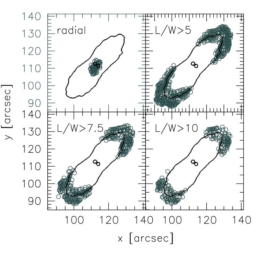
Figure 1: The open circles show the location of the arcs for one of our simulated clusters. The lines common to all panels are the radial and tangential critical lines. The top left panel shows the location of radial arcs while the remaining panels show the tangential arcs for samples selected by their length to width ratios.

5.1.1 Radial and tangential arcs

First, we explore how well the positions of radial and tangential arcs can constrain the location of the respective critical lines. This is clearly shown in the four panels of Fig. 1, where the critical lines for one of our numerically simulated galaxy clusters are shown. The arcs, which we determine from the ray-tracing simulation described above, are shown as open circles in each of the four panels. First, we note that in the top left panel, the radial arcs identified by our criterion are located very close to the radial critical line. The remaining panels show tangential arcs only and these are spread over a thick region surrounding the tangential critical line. We plot only those tangential arcs in each panel which exceed a minimal length-to-width ratio in order to show that the larger the minimal $L/W$ of the arcs chosen, the smaller the spread of arc positions around the critical lines. Second, we note also that tangential arcs tend to form along those parts of the critical curves which are furthest from the cluster centre. The reason for this has been discussed already in some earlier papers (see e.g Bartelmann et al., 1995; Meneghetti et al., 2001). Close to the tangential critical line $\lambda_{\rm t}=1-\kappa-\gamma\sim 0$, hence $\gamma\sim 1-\kappa$. The radial magnification is then $\mu_{\rm r}=\lambda_{\rm r}^{-1}\sim[2(1-\kappa)]^{-1}$. Therefore, the smaller the convergence $\kappa$ is, the more the tangential arcs are radially demagnified, resulting in an arc with a larger length-to-width ratio. Since the convergence is approximately a decreasing function of the cluster-centric distance, tangential arcs with large length-to-width ratio form preferentially close to the critical points at largest distance from the cluster centre.

It is necessary to use tangential arcs with large length-to-width ratios in order to constrain the position of tangential critical curve accurately. However, by choosing those arcs, at least for clusters having elongated or elliptical critical lines, we will constrain only those parts of the critical curves where the convergence is small. As will be discussed in the following sections, this has to be properly taken into account when trying to fit the arc positions to the lens critical curves.

For our analysis we focus on tangential arcs with $L/W>10$. We simulate simultaneous observations of radial and tangential arcs by randomly selecting pairs of radial and tangential images from the arc catalogue generated by our ray-tracing simulations.

5.1.2 Velocity dispersion profiles

As explained in Sect. 4.2, the presence of the BCG is mimicked by simply adding the surface density profile of the galaxy onto that of the cluster. In fact, the growth of the BCG might influence the distribution of the dark matter in the cluster centre and this approximation may be wrong in reality but this is beyond the scope of this paper.

Figure 2: The velocity dispersion profile of one of the galaxy clusters in our sample obtained by combining the best fit density profile of the cluster and the density profile of the BCG. In order for the velocity dispersion profile on scales below $10$ kpc to flatten, the mass of the BCG has been fixed to $10^{12}\,h^{-1}\,M_{\odot}$ within the Jaffe radius. The points indicate the ‘measured’ values that will be used in the fitting procedure. The errorbars mimic observational uncertainties of the measurements.

Since the simulated clusters do not contain stars, we cannot derive the projected velocity dispersion from the simulations. Moreover, velocity dispersion measurements are possible only in the very central part of the cluster up to radii of the order of $\sim 10$ kpc. Despite the high mass resolution, this represents the limit of reliability of the mass profiles which can be inferred from our simulations (Power et al., 2003). Therefore we model the velocity dispersion profiles as follows. First, we fit the density profile of the numerically simulated cluster with a generalised NFW model given by Eq. (8). Then, taking the best fit parameters $(r_{\rm s},\rho_{\rm s},\beta)_{fit}$ we extrapolate the cluster density profile, $\rho_{\rm cl}(r)$, to the inner region, $r<10$ kpc. The BCG density profile is given by Eq. (9). We calculate the enclosed mass $M_{3D}(r)$ by integrating the total density obtained by summing the cluster and the BCG density profiles,

$$M_{3D}=4\pi\int_{0}^{r}(\rho_{\rm cl}+\rho_{\rm BCG})r^{2}{\rm d}r\;.$$ (30)

Finally we derive the projected velocity dispersion profile as described in Sect. 3.4.

As an example, we show in Fig. (2) the simulated velocity dispersion profile for one of the clusters in our sample. The points indicate the constraints used in the following fitting procedure. We assign to each “measurement” an error $\Delta\sigma\sim 40$ km s^-1, mimicking typical observational uncertainties (see e.g. Sand et al., 2004, and references therein).

The density profile of the BCG is fully determined by the mass enclosed by the Jaffe radius. We choose the mass of the BCG so as to produce a velocity dispersion profile which is nearly flat at radii $r\lesssim 10$ kpc, implying that the mass of the BCG is large enough to dominate the cluster centre, as is the case for the galaxy clusters investigated by Sand et al. (2004). At radii much less that the Jaffe radius the Jaffe profile becomes isothermal, $\rho_{\star}\propto r^{-2}$. So if the galaxy dominates the cluster mass at its core, the velocity dispersion profile is expected to be flat close to the cluster centre, and the velocity dispersion is then approximately related to the circular velocity, by

$$v^{2}_{\rm rot}=\frac{GM_{3D}(r)}{r}\;,$$ (31)

by $\sigma_{r}=v_{\rm rot}/\sqrt{2}$

We are able to reproduce flat velocity dispersion profiles in all our clusters by choosing the mass of the BCG in the range $10^{12}\ldots 5\times 10^{12}\,h^{-1}M_{\odot}$. Such masses are compatible with velocity dispersions measured in several BCGs (see e.g. Bernardi et al., 2007).

Figure 3: Distributions of the values of the radial (left panel) and of the tangential (right panel) eigenvalues measured at the positions of the radial and of the tangential arcs found in all the simulations.

5.2 Application to the simulated clusters

From the list of images obtained from the ray-tracing simulations we randomly selected pairs of radial and tangential arcs. As discussed earlier, these are used to constrain the location of the lens critical lines. The complete set of data which we try to fit with our model is then given by the pair of gravitational arcs and by the velocity dispersion profile measured at five different radii in the range $[0-10]\,h^{-1}\,$kpc.

We perform three kinds of fit to the data. Firstly, we repeat the fit made by Sand et al. (2004), assuming axially symmetric lensing potentials while keeping the scale radius of the fitting model fixed at $r_{\rm s}=400\,h^{-1}\,$kpc, and varying the two other parameters: the halo characteristic density $\rho_{\rm s}$ and the inner slope $\beta$. Secondly, we continue to assume axial symmetry, but we let all three parameters be free. Thirdly, we allow for ellipticity in the lensing potential of the fitting model.

For simplicity, we decided not to consider the mass of the BCG as a free parameter in our fits. Moreover, when using elliptical models, we assume we know the ellipticity and the orientation of the iso-contours of the lensing potential by some other means (from other independent observations). Therefore, this fitting model also has only three free parameters, i.e. the parameters characterising the halo density profile. The mass of the BCG and the ellipticity and the position angle of the lens are set to their true values.

The fit is done by minimising a $\chi^{2}$ variable. This is constructed by combining the lensing and the velocity dispersion constraints,

$$\chi^{2}(r_{\rm s},\rho_{\rm s},\beta)=\chi^{2}_{lens}(r_{\rm s},\rho_{\rm s},\beta)+\chi^{2}_{\sigma_{p}}(r_{\rm s},\rho_{\rm s},\beta)\;.$$ (32)

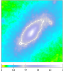
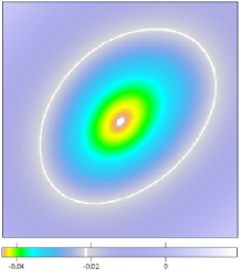
Figure 4: Convergence (left panel) and lensing potential (right panel) of the same cluster whose critical lines are shown in Fig. 1. The side length is $\sim 112^{\prime\prime}$.

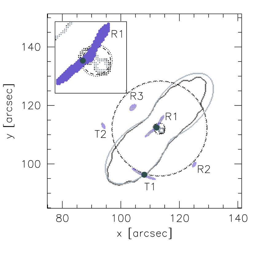
Figure 5: Best fit models for one of the simulated clusters in our sample. The velocity dispersion of the model BCG and our assumed observational error bars are shown in the top panel. The solid line shows the elliptical model fit, the dotted and dashed lines show axially symmetric fits with the scale radius either fixed or free respectively. The bottom panel shows the lens critical lines (black solid lines) and the arcs used to constrain their position (images T1 and R1, marked by the dark-gray dots, indicating the arc centre). A zoom, corresponding to a region of $9"\times 9"$ around the radial arc R1, is displayed in the inset at the upper left corner. The images T2, R2 and R3 are multiple images of the same sources which are lensed into the tangential arc T1 and into the radial arc R1. The velocity dispersion profile and the critical lines of the best fit models, obtained by assuming an elliptical lensing potential, an axially symmetric lensing potential and an axially symmetric lensing potential with $r_{\rm s}=400\,h^{-1}\mathrm{kpc}$, are given by the solid, the dotted and the dashed lines, respectively.

The first term, which concerns the lensing constraints, is defined as follows. The lens critical lines mark the location where the eigenvalues of the Jacobian matrix are zero (see Eq. 7). If we assume that the critical point locations coincide with the arc positions, the best fit model is that which minimises the value of the tangential and radial eigenvalues at the positions of the tangential and radial arcs, respectively. The first term in Eq. (32) is then

$$\chi^{2}_{lens}(r_{\rm s},\rho_{\rm s},\beta)=\left[\frac{\lambda_{t}(r_{\rm s},\rho_{\rm s},\beta)}{\Delta\lambda_{t}}\right]^{2}+\left[\frac{\lambda_{r}(r_{\rm s},\rho_{\rm s},\beta)}{\Delta\lambda_{r}}\right]^{2}\;,$$ (33)

where $\Delta\lambda_{t}$ and $\Delta\lambda_{r}$ reflect the uncertainties in the determination of the critical lines through the position of the radial and tangential arcs. We set $\Delta\lambda_{r}$ and $\Delta\lambda_{t}$ equal to the respective eigenvalues of the Jacobian matrix measured in the numerical simulation at the arc location. This is motivated by the fact that the larger the eigenvalue, the further the position of the arc from the lens critical line. A histogram showing the distributions of the radial and tangential eigenvalues measured at the position of the radial and tangential arcs is shown in Fig. 3. The uncertainty in position is typically larger for radial arcs. Observationally, the determination of the location of the radial critical curve is further complicated by the presence of the BCG, which prevents the detection of radial images close to the cluster centre. In this paper, we neglect this problem, and use all the radial images, even those which might be impossible to observe due to the light of the BCG. Note that our definition of $\chi^{2}_{lens}$ differs from that adopted by other authors. Sand et al. (2004) directly fit the position of the lens critical line determined visually from the arc properties. In practice, the two methods should lead to the same result. Observationally, the estimation of the errors $\Delta\lambda_{t}$ and $\Delta\lambda_{r}$ is difficult and requires calibration with numerical simulations. On the other hand, by fitting the tangential and the radial eigenvalues, instead of the location of the critical line, the required computing time is substantially reduced, which is mandatory since we repeat the analysis on thousands of virtual lensing systems. We defer a more detailed comparison with the results of Sand et al. (2004) to a subsequent section.

The second term in Eq. (32) is given by

$$\chi^{2}_{\sigma_{p}}=\sum_{i}\left[\frac{\sigma_{p,i}-\hat{\sigma}_{p,i}(r_{\rm s},\rho_{\rm s},\beta)}{\Delta\sigma_{p}}\right]^{2}\;,$$ (34)

where $\sigma_{p,i}$ and $\hat{\sigma}_{p,i}$ denote the measured and the expected values of the velocity dispersion at the radius $\xi_{i}$, respectively, and the sum is over all the available measurements of $\sigma_{p}$. As previously stated, the uncertainty in the measurement of the velocity dispersion is fixed at $\Delta\sigma_{p}=40$ km$s^{-1}$.

We find the set of profile parameters, $(r_{\rm s},\rho_{\rm s},\beta)$, which minimises $\chi^{2}$. We repeat the same calculations for $100$ pairs of radial and tangential arcs, obtaining $100$ different “best fit” determinations of the cluster density profiles.

As stated earlier, when fitting with the elliptical model, we assume we know the ellipticity and the position angle of the iso-contours of the lensing potential. These are measured in the simulations by finding the principal axes of the cluster’s lensing potential as follows. We first evaluate the lensing potential on a grid of $N_{g}=1024\times 1024$ points by inverting Eq. (3). Then, we calculate the tensor

$$\Psi_{ij}=\sum_{k}^{N_{g}}\psi_{k}(\mbox{\boldmath$x_{\mit k}$}^{2}\delta_{ij}-x_{k,i}x_{k,j})\;,$$ (35)

where $k$ labels the grid cells, $x_{k}$ is the position vector of the $k$-th cell, with components $x_{k,i}$, $\psi_{k}$ the corresponding value of the lensing potential and $\delta_{ij}$ is the Kronecker delta. The eigenvectors and the eigenvalues of the tensor $\Psi_{ij}$ give the orientation and the ellipticity of the iso-contours of the lensing potential. Since both ellipticity and orientation change with radius, we only consider the region enclosing the lens critical lines.

Figure 6: The thick and the thin solid lines show the tangential and the radial eigenvalues along the lines connecting the cluster center to the arcs T1 and R1 of Fig. 5. The plot zooms over a region of $\pm 1"$ around the tangential and the radial critical lines. The thick and thin dotted horizontal lines correspond to $\Delta\lambda_{t}=\pm 0.01$ and $\Delta\lambda_{r}=\pm 0.03$, respectively.

When applying the method to real clusters, the ellipticity and position angle of the lens should be treated as free parameters. However, to reduce the computational requirement for our simulations, we will assume that these are known quantities. In some cases, stringent constraints on the cluster shape in the central regions, i.e. around the critical lines, can be derived from complementary observations. For example, in the case of relaxed objects, constraints can be imposed from the $X$-ray emission of the intracluster gas which, assuming that the gas is in hydrostatic equilibrium, gives the most direct probe of the projected gravitational potential. However, the equilibrium assumption may be a poor approximation in many cases. An alternative approach would be to combine weak and strong lensing data in order to reconstruct the cluster potential (Bradac et al., 2004; Cacciato et al., 2006). Indeed, recent numerical tests demonstrate that non-parametric methods can be used to measure the lensing potential with enough accuracy (see e.g. Cacciato et al., 2006).

Table 1: The best fit parameters for the cluster shown in Fig. 4, found by using the constraints showed in Fig. 5.

	$r_{\rm s}$	$\rho_{\rm s}$	$\beta$	$\chi^{2}$/dof
	[$h^{-1}$ kpc]	[$h^{2}\,M_{\odot}\,\mathrm{Mpc}^{-3}$]
input model	$224$	$3.54\times 10^{15}$	$0.88$
elliptical fit	$262$	$3.30\times 10^{15}$	$0.83$	0.925
axially sym. fit	$260$	$1.29\times 10^{16}$	$0.11$	1.976
$r_{\rm s}$ fixed fit	$400$	$7.84\times 10^{15}$	$0.13$	2.094

5.3 Regular clusters

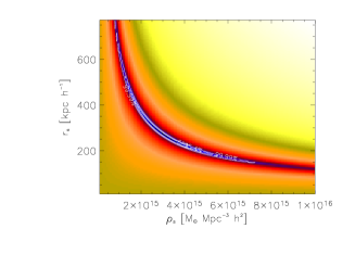
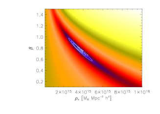
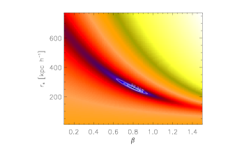
Figure 7: Confidence levels in the $\rho_{\rm s}-r_{\rm s}$, $\rho_{\rm s}-\beta$ and $\beta-r_{\rm s}$ planes (left, central and right panels, respectively). The input model is the cluster illustrated in Fig. 4. The ‘observational’ constraints used are displayed in Fig. 5. The contours corresponding to probability levels of $68.3\%$, $95.4\%$ and $99.7\%$ are shown by the light curves.

We now discuss the results obtained by analysing our simulated clusters. We have divided the cluster sample into two sub-samples. In this subsection we consider only clusters whose mass distribution in the inner region, critical for strong lensing, shows no evidence of substructure. We refer to these as “regular” clusters. In the next subsection we consider the remainder which have perturbed core regions. We call this subsample the “peculiar” clusters.

Regular clusters typically have a lensing potential whose iso-contours can be well fit with ellipses. These clusters are ideal for applying our method. Before showing the overall properties of regular clusters, we first discuss in detail a particular example.

Fig. 4 shows the convergence map and lensing potential for the same object featured in Fig. 1 where the positions of the critical lines are displayed. Fig. 5 shows the best fit velocity dispersion profile (top panel) and critical lines (bottom panel) of this cluster, obtained by fitting the pair of arcs marked by the dark-gray dots (T1 and R1) and the velocity dispersion data given by the black dots with errorbars. A summary of the best fit parameters, compared to their true values, is given in Table 1.

The results show the importance of taking into account the ellipticity when fitting the velocity dispersion and the lensing data. This cluster is well described by a lensing potential with an ellipticity $e=0.33$ and position angle $\theta=46\deg$. The pair of arcs was chosen to provide a good constraint on the position of the critical lines ($\Delta\lambda_{r}\sim 0.03$, $\Delta\lambda_{t}\sim 0.01$). When a model with the appropriate ellipticity for the lensing potential is used, the best fit parameters turn out to be very close to the true values for the simulated cluster (see Table 1). The predicted position of the lens critical lines and the velocity dispersion profile are also in excellent agreement with the true ones. If axial symmetry is assumed however, the fit is totally wrong. In particular, the inner slope of the density profile is grossly underestimated ($0.11-0.13$ instead of $0.88$).

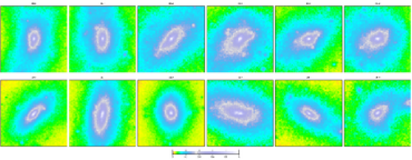
Figure 8: Convergence maps of the clusters classified as “regular”. The side-length of each panel is $226^{\prime\prime}$.

We can interpret this result as follows. The mass within the inner region of the cluster is constrained by the velocity dispersion data. This implies that the central surface density is approximately fixed. At the position of the tangential arc $\kappa+\gamma\sim 1$. Imposing axial symmetry while keeping the same density profile strongly reduces both $\kappa$ and $\gamma$ at the position of the arc, and the tangential critical line moves inward. In order to generate a critical line which still passes through the arc, the axially symmetric model is forced to have a larger projected mass within the circle passing through the arc. This requires a larger mean surface density inside the tangential critical line. But, since the surface density at the cluster centre is fixed, the parameters adjust themselves to flatten the surface density profile. The flattening is limited only by the constraint given by the position of the radial arc. Indeed, the radius of the radial critical curve tends to become larger as $\beta$ becomes smaller. Since for the case shown in Fig. 5 the constraints on the position of the critical lines are strong, the best fit is obtained at the expense of the weaker velocity dispersion constraints (and results in a larger $\chi^{2}$, as given in the last column of Table 1). Thus the recovered best fit density profile is characterised by the smallest central density which is still compatible with the data. This keeps the size of the radial critical line small. The resulting velocity dispersion profile for the axially symmetric fit generally underestimates the true profile. With weaker constraints imposed by the tangential and radial arcs, the best fit axially symmetric model will be generally characterised by larger values of $\beta$.

To simplify the comparison between the positional uncertainties of the critical lines and the errors used in our implementation of $\chi^{2}_{lens}$, we show in Fig. 6 the profiles of the tangential (thick line) and of the radial (thin line) eigenvalues along the lines connecting the cluster center to the arcs T1 and R1 of Fig 5, as derived from the ray-tracing simulation. We zoom into a region of width $\pm 1"$ around the critical lines. We see that the interval $\Delta\lambda_{t}\sim\pm 0.01$ (thick dotted lines) corresponds to $\pm 0.3"$ around the tangential critical line. Similarly, $\Delta\lambda_{r}\sim\pm 0.03$ corresponds to an uncertainty $\pm 0.45"$ in the position of the radial critical line. Such uncertainties are well in agreement with typical errors on the position of arcs (see e.g. Table 3 of Sand et al., 2004).

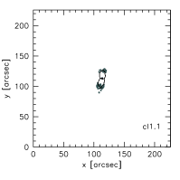
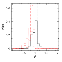
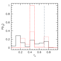
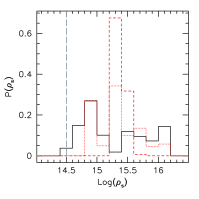
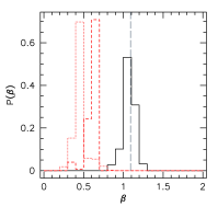
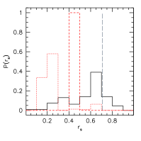
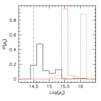
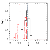
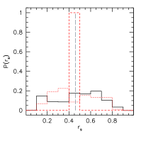
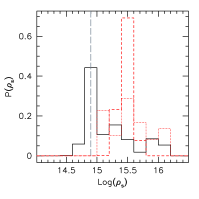
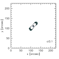
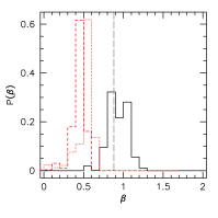
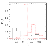
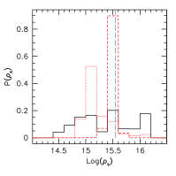
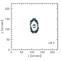
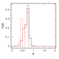
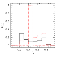
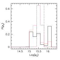
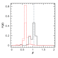
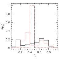
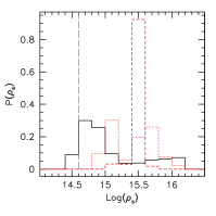
Figure 9: First column: critical lines of six of the clusters classified as “regular”. Gray dots indicate the position of tangential and radial arcs found in the ray-tracing simulations and used in our analysis. Second to fourth column: probability distribution functions of $\beta$, $r_{\rm s}$ and $\rho_{\rm s}$ resulting from constraining the galaxy cluster density profiles using couples of radial and tangential arcs combined with velocity dispersion data. Solid, dotted and short-dashed histograms refer to elliptical, axially symmetric and axially symmetric with fixed $r_{\rm s}=400\,h^{-1}\,\mathrm{kpc}$ fitting models, respectively. The dashed vertical line in each case indicated the true value of the corresponding parameter in the simulation.

An important question is how well can we constrain each of the three parameters characterising the cluster density profile, at least using an appropriate elliptical model. We expect considerable degeneracy especially between the parameters $\rho_{s}$ and $r_{s}$, since both the lensing and the velocity dispersion data provide constraints in a region typically well inside the scale radius. In Fig. 7, we show the confidence levels in the $\rho_{\rm s}-r_{\rm s}$, $\rho_{\rm s}-\beta$ and $\beta-r_{\rm s}$ planes, for the same cluster as above. In each panel we have fixed the remaining parameter to its best fit value, in order to show the degeneracy that remains even after reducing the number of free parameters in the model. Even with good constraints on the position of the lens critical lines there is a strong degeneracy between $r_{\rm s}$ and $\rho_{\rm s}$: for any value of $\rho_{s}$ in the range $(10^{15}-8\times 10^{15})\,M_{\odot}\,\mathrm{Mpc}^{-3}\,h^{2}$ there is a corresponding value of $r_{\rm s}$ in the range $(200-800)~{}\mathrm{kpc}\,h^{-1}$ which produces a good fit. However, $\beta$ appears to be much better constrained. Therefore, unless extremely precise measurements of the position of the lens critical lines are made, the only parameter of the three-dimensional cluster density profile which is likely to be well constrained using this method is the inner slope $\beta$.

As stated earlier, the experiment illustrated above has been repeated for $100$ pairs of radial and tangential arcs for each cluster. The probability distribution functions for some of the cluster projections which have been classified as “regular” are shown in Fig. 9. Note that, differently from what was done in Fig. 7, the probability distribution functions are now marginalized, i.e. we do not fix any parameter to its best fit value. In all the panels, the vertical long-dashed lines indicate the “true” values of the parameters found by fitting Eq. (8) to the three-dimensional density profile of the cluster. While, as discussed earlier, the scale radius $r_{\rm s}$ and characteristic density $\rho_{\rm s}$ are poorly constrained due to the strong degeneracy between these two parameters, in nearly all the cases which we have studied the probability distribution functions of the inner slope $\beta$ have peaks which coincide with the true values, if a lensing potential with the appropriate ellipticity and position angle are used to model the cluster. On the other hand, using axially symmetric models generally leads to underestimate the value of $\beta$.

The discrepancy between the true and the most probable $\beta$ when fitting axially symmetric models is expected to correlate with the ellipticity of the cluster lensing potential. Fig.10 illustrates this dependence on the ellipticity. We plot the medians of the probability distribution functions of $\beta$ for all clusters classified as “regular” as a function of the ellipticity of the cluster lensing potential. The medians have been normalised to the best-fit slope $\beta_{fit}$ of each simulated cluster. The left and the middle panels refer to the fit with axially symmetric lenses, with the scale radius considered as a free parameter or assumed to be fixed, at $r_{\rm s}=400\,h^{-1}$kpc respectively. The right panel shows the results obtained adopting a model with the correct ellipticity and orientation for the lensing potential iso-contours. The errorbars show the interquartile range of each distribution. Under the assumption of axial symmetry, the measured slope is consistent with the true one only for the cluster model with the smallest ellipticity; it is underestimated by $\sim 20-70\%$ for cluster models where a larger $e$ was measured. Unfortunately, most of our clusters have ellipticities in the range $[0.2-0.4]$ and we have only one case with $e\sim 0.15$. On the basis of these results it is difficult to determine the threshold below which the ellipticity can be ignored and an axially symmetric lens model safely used. A larger number of simulated clusters with small ellipticity would be necessary for this purpose. For example, for the cluster cl6.2, which has $e=0.15$, we obtain a good estimate of $\beta$ even when fitting an axially symmetric lens model, but for the cluster cl2.3, which has an ellipticity only slightly larger, $e\sim 0.2$, the slope is underestimated by $\sim 20-35\%$ with the axially symmetric model. On the other hand, when elliptical models are fit, all the measured values of $\beta$ are consistent with their true values.

Figure 10: Medians of the probability distribution functions of the inner slopes for all the clusters classified as “regular” as a function of the ellipticity of the lensing potential. The medians are normalised to the best-fit inner slope $\beta_{fit}$ of each cluster. The error bars are given by the interquartile ranges of the distributions. Each panel corresponds to one of the model fits discussed in the text.

Finally, we show in Fig.11 the probability distribution function of the inner slope obtained by averaging over all the clusters in this subsample. The resulting $P(\beta)$ obtained using elliptical lens models peaks around unity, in agreement with the mean value of $\beta_{fit}$ for our cluster sample, $\overline{\beta}_{fit}\sim 0.95$. The distributions obtained by fitting with axially symmetric lens models have a maximum at $\beta\sim 0.6$.

5.4 Peculiar clusters

The second subsample contains the clusters which we classified as “peculiar”. The convergence maps of these halos are shown in Fig. 12. Visually it is clear that there is likely to be some difficulty in applying the (pseudo-)elliptical lens models to these clusters. The critical lines are very asymmetric, mainly as a result of disturbances due to the passage of large mass concentrations through the cluster core during merger events.

Applying the method to these perturbed clusters generally leads to incorrect results for the determination of the parameters characterising their density profiles. For such clusters a more detailed mass modelling of the lens, including multiple mass components, is necessary in order to reproduce the shape of the critical lines and the positions where arcs form. The shear fields produced by secondary mass concentrations cause the critical lines to be extended in the direction connecting the cluster centre with the perturbing mass clump and usually enhance a cluster’s ability to produce both radial and tangential gravitational arcs, as discussed by Torri et al. (2004).

We show examples of the critical lines and distributions of the inner slope for some peculiar clusters in Fig. 13. Massive substructures distort the shape of the iso-contours of the lensing potential, stretching and elongating them along preferred directions. If such substructures happen to be aligned with the major axis of the main cluster clump, the ellipticity of their lensing potential is generally overestimated, when using a single component lens model. This occurs for example in cluster cl4.3. To compensate for such an overestimate ellipticity, the probability distribution function of the inner slope shifts towards high values of $\beta$. In the previous section we argued that the inner slope is underestimated if an intrinsically elliptical lens is fit with an axially symmetric model. Similarly, $\beta$ is overestimated when a model with too large ellipticity is used to describe a cluster of moderate ellipticity. Again, the central density is constrained by the velocity dispersion data. Tangential arcs form where $\kappa+\gamma\sim 1$. If the ellipticity of the lens is overestimated, the shear $\gamma$ will be overestimated as well. As a result, the convergence $\kappa$ needs to be reduced, implying that the cluster density has to be a steeper function of distance from the centre.

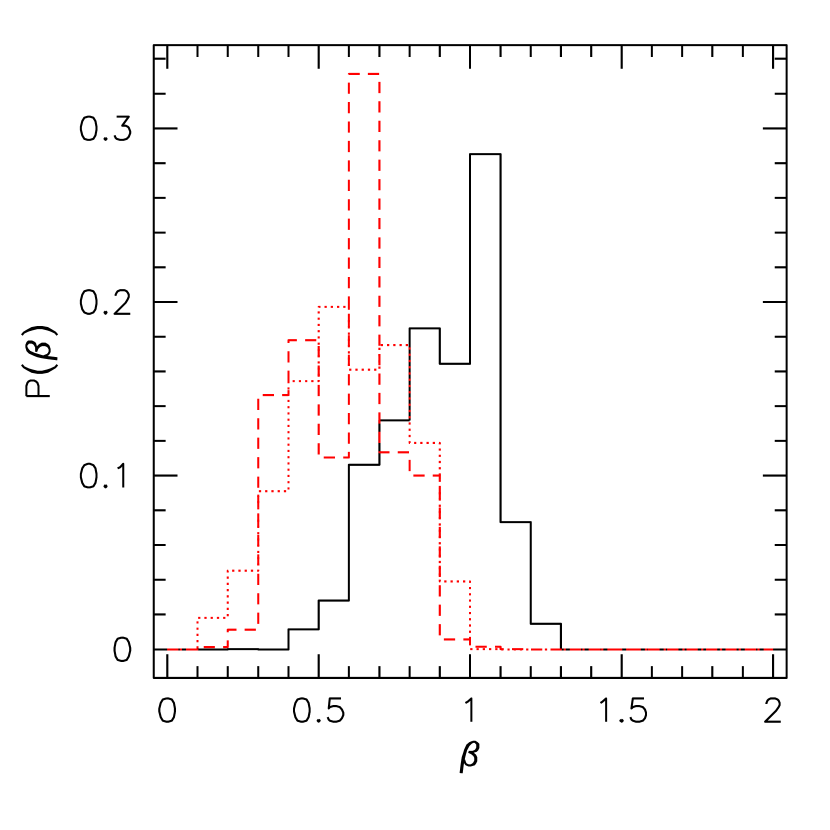
Figure 11: Averaged probability distribution function for the sub-sample of “regular” clusters. Solid, dotted and short-dashed histograms refer to elliptical, axially symmetric and axially symmetric with $r_{\rm s}=400\,h^{-1}\,\mathrm{kpc}$ fitting models, respectively.

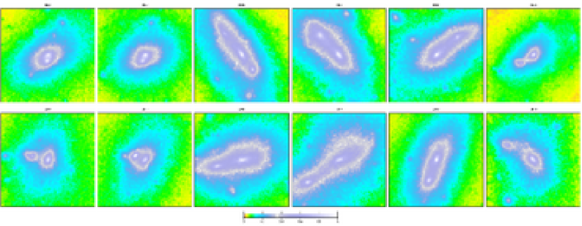
Figure 12: Convergence maps of the clusters classified as “peculiar”. The side-length of each panel is $226^{\prime\prime}$.

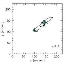
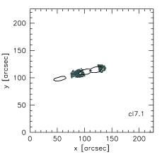
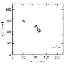
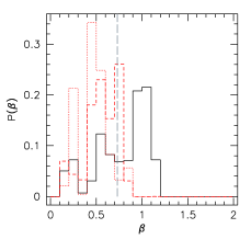
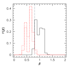
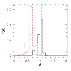
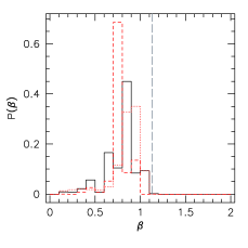
Figure 13: Analysis of some peculiar clusters. Top panels: critical lines and arc positions for clusters cl4.3, cl7.1, cl8.3 and cl5.3. Bottom panels: probability distribution functions of the inner slope. The line types are the same as fig. 9

Less massive or more distant substructures have a smaller impact on the reliability of the method. For example, cluster cl7.1 is less sensitive to the perturbation of a secondary mass clump whose presence is evidenced by a secondary critical line. The resulting probability distribution function of the inner slope is still shifted towards large $\beta$, but less significantly so than for cluster cl4.3. Finally, the substructure in the cluster cl5.3 is too small to affect the shape of the cluster critical lines. The distribution of $\beta$ for this cluster peaks at its correct value.

For some other clusters, however, the opposite results are found. For example in cluster cl8.3, substructures close to the cluster core and not aligned with the major axis of the cluster mass distribution mimic an axially symmetric lensing potential. Consequently, the inner slope if the cluster density profile results to be underestimated, when our method is applied.

6 Comparison to previous observational work

We now discuss the implications of our analysis for the results obtained previously by Sand et al. (2004) for a sample of real clusters. In the preceding sections, we have demonstrated the importance of taking ellipticity and substructures into account in order to derive a correct measurement of the inner slope of density profiles for a set of clusters randomly chosen from a cosmological simulation. Since the number of lenses available in the simulation is not large enough, we were not able to sample uniformly the parameter space of clusters. In particular, our clusters cover a range of ellipticities between $\sim 0.15$ and $\sim 0.4$. Only for one cluster projection, could we measure an ellipticity below $0.2$. Interestingly, for this particular lens, the ellipticity derived from fitting the simulated lensing and velocity dispersion data is in good agreement with the true ellipticity even under the assumption of axial symmetry.

In their work, Sand et al. (2004) carefully chose a set of clusters which appear very round and relaxed, both in optical and X-ray images. For the three clusters in their sample containing both radial and tangential arcs, MS2137.3-2353, A383, and RXJ1133, the ellipticity is presumably in the range $0.1-0.2$ (Gavazzi et al., 2003; Miralda-Escude, 2002; Smith et al., 2001), as Sand et al. (2004) quote in their paper.

Unfortunately, as shown in Fig. 10, there is substantial scatter in the inferred values of the inner slope even for clusters classified as ‘regular” and this makes it difficult to establish the minimum value of the ellipticity for which fitting an axially symmetric model, as Sand et al. (2004) did, would strongly bias the results. A more quantitative comparison with the results of Sand et al. would require a larger number of cluster projections with low ellipticities. Furthermore, as we pointed out earlier, there are some methodological differences between our analysis and that performed by Sand et al. Our definition of $\chi^{2}_{lens}$ differs from theirs in that they fit the location of the critical line whereas we fit the eigenvalues of the Jacobian matrix at the positions of the arcs. In one sense, the two approaches are equivalent, since they both require that the lens critical lines should pass close to the radial and tangential arcs. On the other hand, our estimate of the errors, based on the Jacobian eigenvalues, would require calibration with analytical models before it can used with observational data.

Finally, in our previous analysis, we have used all the radial arcs found in the simulations, regardless of their position relative to the BCG. As we have already mentioned, several of these arcs are probably undetectable in real observations, because they are too close to the cluster centre and thus would be completely embedded in the light of the dominant galaxy. In the case of elliptical radial critical lines, i.e. when the lenses are elliptical, this implies that those sections of the critical line reaching farthest from the cluster centre would be more easily traced by lensing observations. Assuming axial symmetry in these cases would be quite dangerous and potentiall have a strong effect on the determination of the inner slope. Indeed, steep density profiles produce small radial critical lines due to the large curvature of the time delay surface at the central maximum.

In order to overcome some of these difficulties in comparing our results to those of Sand et al. we have performed a different set of simulations. We choose one of the clusters in our sample, cluster cl1, which is the strongest lens, and project it along 400 different lines-of-sight with direction uniformly distributed on the surface of a sphere centred on the cluster BCG. We carry out simulated lensing measurements on each of the projections. The ellipticity of the lensing potential in the different projections varies between $\sim 0$ and $\sim 0.5$, indicating that the cluster is highly triaxial. The measured ellipticity for each of the 400 projections are plotted as a scatter diagram in the left panel of Fig. 14.

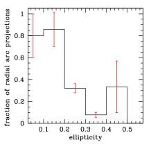
Figure 14: Left panel: ellipticities of the lensing potential for 400 different projections of the cluster cl1. The projections which give rise to both radial and tangential arcs are indicated by filled circles. Right panel: fraction of radial arc projections per ellipticity bin.

An interesting property of this cluster is that most projections characterized by small ellipticities of the lensing potential are able to produce both radial and tangential arcs. We quantify this in the right panel of Fig. 14, where we show the fraction of projections with radial and tangential arcs (and the corresponding errorbars) per ellipticity bin. We see that for ellipticities below 0.2 more than $80\%$ of the projections produce radial arcs in addition to tangential arcs. Such projections correspond to viewing the cluster nearly along its major axis.

Compared to our previous, more general approach, we now tailor the criteria for selecting radial and tangential arcs and for estimating position errors to the procedures adopted by Sand et al. The aim is to mimic the observational process as closely as possible. Firstly, we use only radial arcs lying at distances larger than $4\,h^{-1}$kpc from the cluster centre, which is the minimal distance of the radial arcs in the cluster sample used by Sand et al. Secondly, we use only those arcs arising from mergers of multiple images of the same source, i.e. arcs that in the observations would have multiple brightness peaks. These are identified in the simulations by mapping the centre of each source galaxy onto the lens plane. We use the multiple peaks along the same arc to obtain realistic measurements of the positions, $x_{c}^{t,r}$, of the tangential and of the radial critical lines and to estimate the errors $\Delta x_{c}^{t,r}$. The former are determined by finding the intermediate points between two close peaks with inverse image parity (opposite sign of the magnification). The latter are estimated by measuring the distance between the same brightness peaks. For fitting these data, we define a new $\chi^{2}_{lens}$ variable that is completely consistent with that used by Sand et al.,

$$\chi^{2}_{lens}(r_{\rm s},\rho_{\rm s},\beta) = \left[\frac{x_{c}^{t}-\hat{x}_{c}^{t}(r_{\rm s},\rho_{\rm s},\beta)}{\Delta x_{c}^{t}}\right]^{2}$$ (36)

$$+ \left[\frac{x_{c}^{r}-\hat{x}_{c}^{r}(r_{\rm s},\rho_{\rm s},\beta)}{\Delta x_{c}^{r}}\right]^{2}\;,$$

where $\hat{x}_{c}^{t,r}$ denote the expected positions of the tangential and the radial critical lines, given a set of input parameters $(r_{\rm s},\rho_{\rm s},\beta)$.

The model cluster used for this new set of simulations is not able to produce arcs which meet the selection criteria in all its projections. As a result, we can only use a subsample of them; these are identified by the filled circles in Fig. 14. The vast majority is characterised by ellipticities below $0.3$. In particular, we now have $\sim 70$ projections whose lensing potential has an ellipticity less than $0.2$.

For each projection, we fit all possible combinations of radial and tangential arcs found in the simulations that meet the selection criteria. This is done by minimising the $\chi^{2}$ variables in Eqs. 36 and 34 and by assuming axial symmetry, as was done by Sand et al. In order to perform a direct comparison with the analysis of Sand et al., we also centre the innermost bin of the simulated velocity dispersion profile on $R=0.4\,h^{-1}$kpc, and extend the measurements to $R=5\,h^{-1}$kpc with a total of four equidistant bins.

Figure 15: Mean inner slopes in different bins of the ellipticity of the lensing potential. These are estimated by fitting with axially symmetric models all the possible pairs of radial and tangential arcs produced by many projections of cluster cl1. The values of $\beta$ are normalised to the best-fit inner slope $\beta_{fit}$. The errorbars show 3$-\sigma$ statistical errors.

Each determination of $\beta$ is normalised to the best-fit inner slope $\beta_{fit}$ of cluster cl1. The estimates are divided into equidistant ellipticity bins of size $\sim 0.03$. In each bin, we calculate the mean value of the normalised inner slopes, weighting each measurement with the corresponding $\chi^{2}$. The resulting mean normalised $\beta$ is shown as a function of the ellipticity of the lensing potential in Fig. 15. The errorbars give the 3$-\sigma$ statistical errors.

The results are in good agreement with those previously discussed in Sect. 5. Firstly, changing the definition of $\chi^{2}_{lens}$, in line with that adopted by Sand et al. does not modify our conclusions either qualitatively or quantitatively. The inner slope is underestimated when the model used to fit the data is axially symmetric. Secondly, we find that it is possible to underestimate the inner slope even in cases where the lensing potential has very low ellipticity. Indeed, for ellipticities between $0$ and $0.15$, the inner slopes inferred by assuming axial symmetry are typically $10-35\%$ smaller than the true ones.

The joint probability distribution function of the inner slope of the clusters in the sample studied by Sand et al. peaks at $\beta=0.52_{-0.5}^{+0.5}$ (68% CL). Taking into account several possible systematic effects, such as anisotropy of the stellar orbits, an incorrect choice of scale radius or of the luminous mass model, this best-fit value may be shifted by $\sim 0.2$ (see the discussion on systematics in Sect. 6 of Sand et al.). Thus, we conclude that our results for axially symmetric fitting models are compatible with those of Sand et al. Our results indicate that the small values of the inner slope that they estimate from their cluster sample can be explained by the effects of the small but non-zero ellipticity of the lenses.

We also note that the joint probability distribution function found by Sand et al. is strongly conditioned by two clusters, MS2137.3-2353 and A383. Existing two-dimensional mass reconstructions of these two lenses, based on the NFW density profile, indicate that these clusters have very small scale radii ($\sim 60\,h^{-1}$kpc) (see e.g. Comerford et al., 2006). Thus, any flattenting of their density profile occurs on scales where the BCG already dominates the mass distribution. In such regions, the density profile of the dark matter mass component is likely to be very poorly constrained.

7 Summary and discussion

In this paper we have explored, using numerical simulations, the possibility of constraining the density profiles of galaxy clusters. The method, proposed by Sand et al. (2002,2004), consists of using a two component lens model, comprising a dark matter halo and a central dominant galaxy, to fit the positions of radial and tangential gravitational arcs and the velocity dispersion profile of the cluster BCG. While Sand et al. used axially symmetric models for describing the mass distribution of clusters, we have used a more general pseudo-elliptical lens model, where ellipticity is included in the lensing potential.

Using galaxy clusters obtained from cosmological N-body simulations with high mass resolution and investigating their lensing properties with ray-tracing techniques, we have created mock catalogues of radial and tangential arcs and simulated velocity dispersion profiles. We have fit the data with both the generalised pseudo-elliptical and the axially symmetric lens models. This allowed us to evaluate the reliability of the method and the impact that the ellipticity of the cluster lensing potential has on the correct estimate of the profile parameters. The projected clusters have been divided in two sub-samples: those which do not contain substructure in the inner region are classified as “regular”, while those with perturbed cores are classified as “peculiar”. By comparing the results obtained with the two sub-samples, we have studied the systematic errors due to incorrect modelling of the cluster. In our fit, the cluster density profile is assumed to be a generalised NFW profile, depending on three free parameters, namely the inner logarithmic slope $\beta$, the scale radius $r_{\rm s}$ and the characteristic density $\rho_{\rm s}$.

Our main findings can be summarised as follows:

• If a model with the correct ellipticity and orientation of the iso-contours of the cluster lensing potential is used, the inner slope of the density profile is accurately recovered, at least for those clusters which we classify as “regular”. On the other hand, the scale radius and the characteristic density are poorly constrained, because a strong degeneracy exists between these two parameters.

• When using the axially symmetric lens models to fit the data, the inner slope is generally significantly underestimated. The degree to which $\beta$ is incorrectly determined depends on the ellipticity of the cluster lensing potential, and is larger for larger ellipticities. For our clusters with ellipticities in the range $0.2-0.4$, the inner slopes resulting from axially symmetric fits are $\sim 20\%$ to $\sim 70\%$ smaller than the true values. When averaging over all “regular” clusters , we find that axially symmetric fits typically underestimate $\beta$ by $\sim 40\%$. By contrast, when the cluster ellipticities are properly taken into account, the averaged probability distribution function of the inner slopes is in good agreement with the distribution of the true inner slopes of the density profiles of the clusters in our sample.

• The fit produces incorrect results if applied to clusters whose critical regions for strong lensing are perturbed by massive substructures. i.e. for clusters which are undergoing major merger events and which we classified as “peculiar”. The shear field produced by secondary mass clumps distorts the shape of the lens critical lines and so the position of radial and tangential arcs are badly reproduced by simple lens models. In such cases a more detailed lens model is required. The effect of the substructures depends on their mass and on their location with respect to the main cluster clump. For clusters where massive substructures are located close to the critical regions, the inner slope can be both over- or underestimated. However, in some cases we are able to obtain a good measurement of the inner slope even for relatively perturbed clusters, because the perturbing substructure is too small or too distant from the cluster centre to affect the shape of the lensing potential iso-contours significantly in the region where arcs form.

• A large number of lensing simulations, obtained by projecting the same cluster in 400 different directions, have been performed with the specific aim of determining the range of ellipticities for which the assumption of axial symmetry is applicable. We verify that even for ellipticities below $0.2$, the inner slopes can be underestimated by $\sim 10-35\%$.

We conclude that using strong lensing and velocity dispersion data is potentially a very powerful method for constraining the mass distribution in the inner parts of galaxy clusters, provided that the lensing potential is accurately modelled. In particular, the impact of ellipticity cannot be neglected even for clusters which deviate from axial symmetry only moderately. The effect of substructure in the inner region of clusters also needs to be taken into account.

By neglecting the effects of ellipticity, Sand et al (2002,2004) could be led to underestimate the slope of the inner profiles of the clusters they analysed and to the conclusion that their data disagreed with the predictions of the cold dark matter model. Our analysis shows such a conclusion may be unjustified. At the same time however, it also demonstrates that the general approach pioneered by Sand et al provides a powerful means to probe the central distribution of mass in clusters.

References

- Allen, Ettori, & Fabian (2001) Allen S. W., Ettori S., Fabian A. C., 2001, MNRAS, 324, 877
- Allen, Schmidt, & Fabian (2002) Allen S. W., Schmidt R. W., Fabian A. C., 2002, MNRAS, 335, 256
- Arabadjis, Bautz, & Garmire (2002) Arabadjis J. S., Bautz M. W., Garmire G. P., 2002, ApJ, 572, 66
- Bartelmann et al. (1998) Bartelmann M., Huss A., Colberg J. M., Jenkins A., Pearce F. R., 1998, A&A, 330, 1
- Bartelmann & Meneghetti (2004) Bartelmann M., Meneghetti M., 2004, A&A, 418, 413
- Bartelmann et al. (1995) Bartelmann, M., Steinmetz, M., & Weiss, A. 1995, A&A, 297, 1
- Bernardi et al. (2007) Bernardi, M., Hyde, J.B., Sheth, R.K., Miller, C.J., & Nichol, R.C., 2007, ApJ, 133, 1741
- Bradac et al. (2004) Bradac, M., Schneider, P., Lombardi, M., & Erben, T. 2004, ArXiv Astrophysics e-prints
- Lewis, Stocke, & Buote (2002) Lewis A. D., Stocke J. T., Buote D. A., 2002, ApJ, 573, L13
- Cacciato et al. (2006) Cacciato M., Bartelmann M., Meneghetti M., Moscardini L., 2006, A&A, 458, 349C
- Comerford et al. (2006) Comerford J. M., Meneghetti M., Bartelmann M., Schirmer M., 2006, ApJ, 642, 39C
- Davis et al. (1985) Davis M., Efstathiou G., Frenk C. S., White S. D. M., 1985, ApJ, 292, 371
- Dahle, Hannestad, & Sommer-Larsen (2003) Dahle H., Hannestad S., Sommer-Larsen J., 2003, ApJ, 588, L73
- de Blok, Bosma, & McGaugh (2003) de Blok W. J. G., Bosma A., McGaugh S., 2003, MNRAS, 340, 657
- Diemand, Moore, & Stadel (2004) Diemand J., Moore B., Stadel J., 2004, MNRAS, 353, 624
- Efstathiou, Sutherland, & Maddox (1990) Efstathiou G., Sutherland W. J., Maddox S. J., 1990, Natur, 348, 705
- Ettori & Lombardi (2003) Ettori S., Lombardi M., 2003, A&A, 398, L5
- Gao et al. (2004a) Gao L., De Lucia G., White S. D. M., Jenkins A., 2004, MNRAS, 352, L1
- Gao et al. (2004b) Gao L., White S. D. M., Jenkins A., Stoehr F., Springel V., 2004, MNRAS, 355, 819
- Gavazzi et al. (2003) Gavazzi R., Fort B., Mellier Y., Pelló R., Dantel-Fort M., 2003, A&A, 403, 11
- Gavazzi (2005) Gavazzi R., 2005, A&A, 443, 793G
- Kneib et al. (2003) Kneib J.-P., et al., 2003, ApJ, 598, 804
- Gnedin et al. (2004) Gnedin O. Y., Kravtsov A. V., Klypin A. A., Nagai D., 2004, ApJ, 616, 16
- Hayashi & Navarro (2005) Hayashi E., Navarro J. F., 2005, in preparation.
- Hockney & Eastwood (1988) Hockney R. W., Eastwood J. W., 1988, csup.book,
- Jaffe (1983) Jaffe W., 1983, MNRAS, 202, 995
- Lewis, Buote, & Stocke (2003) Lewis A. D., Buote D. A., Stocke J. T., 2003, ApJ, 586, 135
- Buote & Lewis (2004) Buote D. A., Lewis A. D., 2004, ApJ, 604, 116
- Martel (1991) Martel H., 1991, ApJ, 366, 353
- Miralda-Escude (1995) Miralda-Escude J., 1995, ApJ, 438, 514
- Miralda-Escude (2002) Miralda-Escude J., 2002, ApJ, 564, 60
- Mellier (1999) Mellier Y., 1999, ARA&A, 37, 127
- Meneghetti, Bartelmann, & Moscardini (2003) Meneghetti M., Bartelmann M., Moscardini L., 2003, MNRAS, 340, 105
- Meneghetti, Bartelmann, & Moscardini (2003) Meneghetti M., Bartelmann M., Moscardini L., 2003, MNRAS, 346, 67
- Meneghetti et al. (2000) Meneghetti M., Bolzonella M., Bartelmann M., Moscardini L., Tormen G., 2000, MNRAS, 314, 338
- Meneghetti et al. (2001) Meneghetti M., Yoshida N., Bartelmann M., Moscardini L., Springel V., Tormen G., White S. D. M., 2001, MNRAS, 325, 435
- Moore et al. (1998) Moore B., Governato F., Quinn T., Stadel J., Lake G., 1998, ApJ, 499, L5
- Navarro, Eke, & Frenk (1996) Navarro J. F., Eke V. R., Frenk C. S., 1996, MNRAS, 283, L72
- Navarro, Frenk, & White (1996) Navarro J. F., Frenk C. S., White S. D. M., 1996, ApJ, 462, 563
- Navarro, Frenk, & White (1997) Navarro J. F., Frenk C. S., White S. D. M., 1997, ApJ, 490, 493
- Navarro et al. (2004) Navarro J. F., et al., 2004, MNRAS, 349, 1039
- Power et al. (2003) Power, C., Navarro, J., Jenkins, A., et al. 2003, MNRAS, 338, 14
- Pratt & Arnaud (2002) Pratt G. W., Arnaud M., 2002, A&A, 394, 375
- Pratt & Arnaud (2003) Pratt G. W., Arnaud M., 2003, A&A, 408, 1
- Sanchez et al. (2005) Sanchez A. G., Baugh C. M., Percival W. J., Peacock J. A., Padilla N. D., Cole S., Frenk C. S., Norberg P., astro-ph/0507583.
- Sand, Treu, & Ellis (2002) Sand D. J., Treu T., Ellis R. S., 2002, ApJ, 574, L129
- Sand et al. (2004) Sand D. J., Treu T., Smith G. P., Ellis R. S., 2004, ApJ, 604, 88
- Schmidt, Allen, & Fabian (2001) Schmidt R. W., Allen S. W., Fabian A. C., 2001, MNRAS, 327, 1057
- Schneider et al. (1992) Schneider, P., Ehlers, J., & Falco, E. E. 1992, Gravitational Lenses (Springer Verlag, Heidelberg)
- Simon et al. (2003) Simon J. D., Bolatto A. D., Leroy A., Blitz L., 2003, ApJ, 596, 957
- Simon et al. (2005) Simon J. D., Bolatto A. D., Leroy A., Blitz L., Gates E. L., 2005, ApJ, 621, 757
- Smith et al. (2001) Smith G. P., Kneib J.-P., Ebeling H., Czoske O., Smail I. R., 2001, ApJ, 552, 493
- Spergel et al. (2003) Spergel D. N., et al., 2003, ApJS, 148, 175
- Springel, Yoshida, & White (2001) Springel V., Yoshida N., White S. D. M., 2001, NewA, 6, 79
- Torri et al. (2004) Torri, E., Meneghetti, M., Bartelmann, M., et al. 2004, MNRAS, 349, 476
- van den Bosch & Swaters (2001) van den Bosch F. C., Swaters R. A., 2001, MNRAS, 325, 1017
- Yoshida, Sheth, & Diaferio (2001) Yoshida N., Sheth R. K., Diaferio A., 2001, MNRAS, 328, 669