Spoke Formation Under Moving Plasma Clouds

Abstract

Goertz and Morfill (1983) propose that spokes on Saturn’s rings form under radially moving plasma clouds produced by meteoroid impacts. We demonstrate that the speed at which a plasma cloud can move relative to the ring material is bounded from above by the difference between the Keplerian and corotation velocities. The radial orientation of new spokes requires radial speeds that are at least an order of magnitude faster. The model advanced by Goertz and Morfill fails this test.

1 Introduction

The nature of the “spokes” in Saturn’s rings remains a matter of speculation 25 years after their discovery by the Voyager spacecraft. A brief summary of their properties is given here; for more details see Mendis et al. (1984) and references therein.

1. Spokes are transient radial albedo features superposed on Saturn’s rings.

2. Spokes are composed of dust with a narrow size distribution centered at 0.5 micron.

3. Spokes have optical depths of about 0.01.

4. Spokes are only seen near corotation, which is where the Keplerian angular velocity of the ring particles matches the planet’s rotational angular velocity. Corotation occurs in the outer B ring.

5. Individual spokes measure about 10,000 km in radial length and 2,000 km in azimuthal width; they extend over about 10% of the ring radius.

6. Spokes are seen preferentially on the morning ansa of Saturn’s rings, and are most closely radial there.

7. Spokes fade and are distorted by differential rotation as they move from morning toward evening ansa.

8. A few observations have been interpreted as showing the birth of individual spokes within 5 minutes along their entire lengths. This timescale implies a propagation velocity of at least 20 km s^-1.

9. Spokes are only observed at small ring opening angle to the Sun (McGhee et al. 2005).

The above observations suggest that spoke formation involves the sudden lifting of a radial lane of dust grains from the surface of the rings. Their subsequent fading and distortion is compatible with the elevated dust grains moving on Keplerian orbits that intersect the ring plane half an orbital period (i.e. about 5 hours) later.

Currently the most popular model for spoke formation is that of Goertz and Morfill (1983, GM). GM propose that the formation of a spoke is initiated when a meteoroid impacts the ring and creates a dense plasma cloud. Electrons from the cloud are absorbed by the ring producing a large electric field which levitates negatively charged dust grains. The grains enter the cloud where they absorb additional electrons. Overall charge neutrality is maintained by the net positive charge of the plasma.

Because the dust grains are massive, they move on Keplerian orbits. The plasma in which they are immersed is however tied to the magnetic field lines which pass through the ionosphere of Saturn. The motion of the negatively charged dust relative to the positively charged plasma produces an azimuthal electric field that causes the plasma cloud to drift radially. GM argue that the plasma cloud will continue to levitate dust grains as it moves. According to their calculations, the plasma cloud drifts in the radial direction, away from corotation, at 20 – 70 km/s. This velocity is sufficient to account for the formation of a radial spoke of length 10,000 km within 5 minutes.

We perform a self-consistent calculation of the plasma cloud drift velocity in §2. It establishes that the drift velocity cannot exceed the difference between the local Keplerian and corotation velocities. This upper limit is of order 1 km s^-1 in the region where spokes are observed. We reveal the source of GM’s error in §3 and estimate the correct drift velocity in §4. In §5 we comment on the response of Morfill & Thomas (2005) to these issues. A short summary in §6 concludes our paper.

2 Drift of a Plasma Cloud

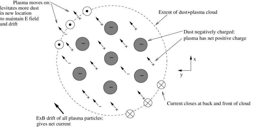
Figure 1: The dusty plasma cloud, viewed from above in the local rest frame of the ring particles.

The essence of GM’s model is illustrated in Fig. 1. The part of the ring plane at the base of the plasma cloud has a finite Hall conductivity: in the presence of an electric field in the local rest frame of the ring particles, the net positively charged plasma will drift relative to the negatively charged dust grains which are embedded within it. Away from the plasma cloud the ring plane has negligible electrical conductivity.

Overall charge neutrality of the dusty plasma implies that currents must close. Although the magnetospheric plasma maintains as equipotentials the magnetic field lines linking the ring plane to the ionosphere, it cannot carry currents across the field lines. Thus currents that flow through the base of the plasma cloud must close in Saturn’s ionosphere. In the wake of the cloud, the levitated dust rapidly combines with the positive ions that balance its charge, leaving the spoke trail behind the cloud non-conducting.

2.1 The model

We analyse a simple model that captures the relevant features of the system of a dusty plasma cloud, ionosphere, and magnetosphere. A 2D strip of material in the $xy$-plane at $z=0$ represents the dust grains (plus neutralizing ions) at the base of the plasma cloud at a given time. Infinite sheets of a different material at $z=\pm L$ take the place of the ionosphere. The magnetosphere consists of a vertical magnetic field of strength $B$ embedded in a massless plasma that maintains the field lines as equipotentials. All calculations are done in the rest frame of the strip relative to which the ionosphere moves with velocity ${\mathbf{v}}=(0,v,0)$ (see Fig. 2). Thus $x$ represents the radial direction in the rings, and $y$ is azimuthal.

We wish to determine the drift velocity of the plasma in and above the strip. This is equivalent to finding the horizontal electric field in the system since the drift velocity ${\mathbf{v}_{p}}$ measured in the same frame as $\bf{E}$ satisfies

$${\bf v}_{p}=c\frac{{\bf E}\times{\bf B}}{B^{2}}\,.$$ (1)

2.2 Finding the drift velocity

In the rest frame of a conducting sheet, the height-integrated current density ${\mathbf{J}}$ perpendicular to the magnetic field is given by

$${\mathbf{J}}=\sigma{\mathbf{E}}+\Sigma\frac{{\mathbf{B}}\times{\mathbf{E}}}{|B|},$$ (2)

where $\sigma$ and $\Sigma$ are, respectively, the height-integrated direct (Pedersen) and Hall conductivities. Because the ionosphere consists of two sheets in parallel, its effective conductivity is twice that of a single sheet.

Subscripts $s$ and $i$ are used to denote properties of the strip and ionosphere. The electric field in the rest frame of the ionosphere is related to that in the rest frame of the strip by

$$E_{xi}=E_{xs}+\frac{vB}{c}\,,\;\;E_{yi}=E_{ys}.$$ (3)

We assume, as GM implicitly did, that the currents are small enough so as not to significantly perturb the externally imposed magnetic field $B$, i.e. $4\pi J/c\ll B$. We also take $v\ll c$.

Then, using Eq. (2) for the currents in the rest frame of each conductor, and expressing current conservation by

$${\mathbf{J}_{s}}+{\mathbf{J}_{i}}=0\,,$$ (4)

we solve the resulting simultaneous equations to give

$$E_{xs}=-\frac{vB}{c}\left[\frac{\Sigma_{i}\Sigma_{t}+\sigma_{i}\sigma_{t}}{\Sigma_{t}^{2}+\sigma_{t}^{2}}\right],$$ (5)

$$E_{ys}=\frac{v|B|}{c}\left[\frac{\Sigma_{s}\sigma_{i}-\Sigma_{i}\sigma_{s}}{\Sigma_{t}^{2}+\sigma_{t}^{2}}\right],$$ (6)

where $\Sigma_{t}=\Sigma_{s}+\Sigma_{i}$ and $\sigma_{t}=\sigma_{s}+\sigma_{i}$.

The velocity ${\mathbf{v}}_{p}$ at which the plasma cloud moves then follows from Eq. (1):

$$v_{px}=v\left[\frac{\Sigma_{s}\sigma_{i}-\Sigma_{i}\sigma_{s}}{\Sigma_{t}^{2}+\sigma_{t}^{2}}\right]b,$$ (7)

$$v_{py}=v\left[\frac{\Sigma_{i}\Sigma_{t}+\sigma_{i}\sigma_{t}}{\Sigma_{t}^{2}+\sigma_{t}^{2}}\right]\,,$$ (8)

where we have introduced $b=B/|B|=\textrm{sign}(B)$.

The main message from Eqs. (7) and (8) is that $|v_{px}|,|v_{py}|<v$. This finding contradicts the result obtained by GM (i.e. $|v_{px}|=20-70\textrm{~{}km~{}s}^{-1}$), because in the region in which spokes appear, $v\lesssim 1\textrm{~{}km~{}s}^{-1}$. The reasons for this discrepancy are detailed in §3.

Another interesting limit is one in which either or both of the direct and Hall ionospheric conductivities are much larger than both components of the strip’s conductivity. In this case, $|v_{px}|\ll v$ and $v_{py}\approx v$; i.e., the plasma cloud basically corotates with the ionosphere.

3 Where GM Erred

GM neglected several terms when solving equations analogous to our Eqs. (1)–(4). The components of the height integrated currents in both the strip and ionosphere as a function of the electric fields in their respective rest frames satisfy:

$$J_{xs} = [\sigma_{s}E_{xs}]-[b\Sigma_{s}E_{ys}]$$ (9)

$$J_{ys} = [\sigma_{s}E_{ys}]+b\Sigma_{s}E_{xs}$$ (10)

$$J_{xi} = \sigma_{i}E_{xi}-[b\Sigma_{i}E_{yi}]$$ (11)

$$J_{yi} = \sigma_{i}E_{yi}+[b\Sigma_{i}E_{xi}]\,.$$ (12)

Terms left out in GM’s analysis are enclosed in square brackets. Since the strip has negligible direct conductivity, neglecting terms proportional to $\sigma_{s}$ does no harm. The Hall current in the ionosphere should be included since the Hall conductivity is comparable to the direct conductivity in the ionosphere. However, this neglect is not a large source of error. The serious omission is that of the strip’s Hall current from $J_{xs}$, as indicated in Eq. (9).

The above equations, with the bracketed terms omitted, yield the incorrect result

$$v_{px}=v\frac{\Sigma_{s}}{\sigma_{i}}b\,,$$ (13)

from which $|v_{px}|>v$ follows for $|\Sigma_{s}|>\sigma_{i}$.

Physically, GM’s error is described by their incorrect statement that “the motion of the plasma cloud does not constitute a perpendicular (to ${\mathbf{B}}$) current as the plasma cloud is charge neutral”. Because the dust grains are negatively charged the plasma must have a net positive charge. The azimuthal electric field set up by the differential motion of the plasma and the dust grains does cause the plasma to drift radially, but because the plasma is net positive, this constitutes a radial Hall current. This radial current closes in the ionosphere, and thus modifies the radial electric field in both the ionosphere and the strip. But the radial electric field is responsible for driving the azimuthal Hall current in the strip, and this modification is not taken into account in GM. They therefore incorrectly fix $v_{py}=v$, leading to a severe overestimate of $v_{px}$. All these factors are accounted for in the self-consistent calculation outlined in §2.

4 Recalculation of Drift Velocity

We recalculate the drift velocity of a plasma cloud from Eqs. (7) and (8).

The direct conductivity in the strip is very small because the dust grains have low mobility and the plasma is tied to the magnetic field lines. The Hall conductivity, which results from the ${\bf E\times B}$ drift of the positively charged plasma, is correspondingly high, of order

$$\Sigma_{s}\sim-\frac{N_{p}ec}{|B|}\,,$$ (14)

where $N_{p}e$ is the height integrated charge density of the plasma. Using the approach of GM, we estimate the height integrated charge density to be of order $10^{1}$ esu cm^-2, which gives $\Sigma_{s}\sim-10^{14}\textrm{~{}cm~{}s}^{-1}$.

Saturn’s ionospheric conductivities vary with latitude and with time, with typical dayside values of the height-integrated direct conductivity being $\sigma_{i}\simeq 10^{12}-10^{13}\textrm{~{}cm~{}s}^{-1}$, and nightside values about 100 times smaller (Cheng and Waite 1988). The Hall conductivity is about an order of magnitude smaller, e.g. for the auroral region we have $\sigma_{i}=5\times 10^{13}\textrm{~{}cm~{}s}^{-1}$ and $\Sigma_{i}=8\times 10^{12}\textrm{~{}cm~{}s}^{-1}$ (Atreya et al. 1983). The direct current is carried predominantly by protons, and the Hall current by electrons, which suffer fewer collisons per gyroperiod than the protons, so ${\bf E\times B}$-drift more freely. Collision frequencies of electrons and protons in Saturn’s ionosphere are smaller than the respective gyrofrequencies, so the Hall conductivity is smaller than the direct conductivity.

We substitute into Eqs. (7) and (8) the typical dayside values $2\sigma_{i}=1\times 10^{13}\textrm{~{}cm~{}s}^{-1}$ and $2\Sigma_{i}=1\times 10^{12}\textrm{~{}cm~{}s}^{-1}$ (the factors of two account for both hemispheres of the ionosphere, although we note that we do not expect north-south symmetry of conductivities). We then obtain

$$v_{px}=6\times 10^{-2}v,\;v_{py}=-2\times 10^{-3}v,$$ (15)

where we have used $b=-1$ as is appropriate for Saturn, and where $v\lesssim 1$ km/s. With these velocities, spokes will not form quickly or radially. The strip Hall conductivity is high enough to drag the plasma column in an almost Keplerian orbit.

5 Discussion

In response to this paper, Morfill & Thomas (2005) revisit the GM model for spoke formation. They provide further details about dust charging and plasma cloud structure. These details are however irrelevant to the criticisms raised here, and make no difference to the fact that, just as the radial electric field produces an azimuthal Hall current, an azimuthal electric field will produce a radial Hall current. These currents and electric fields must be treated self-consistently, resulting in the conclusions reached in this paper.

6 Conclusions

We have studied the physical situation in which a strip of conducting material moves between two parallel sheets of a different material, to which it is joined by perpendicular magnetic field lines (Fig. 2). The plasma on these field lines will drift in the plane of the strip, both parallel and perpendicular to the relative velocity vector. We have shown that the magnitude of this drift velocity cannot exceed that of the relative strip-sheet velocity.

Application of this limit to the most popular model for spoke formation demonstrates that the model rests upon a gross overestimate of the velocity at which a plasma cloud can drift.

7 Acknowledgments

This research was supported by NSF grant AST 00-98301. We thank J. H. Waite for information on Saturn’s ionospheric conductivity.

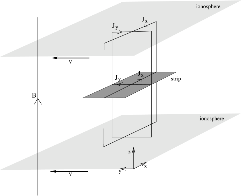
Figure 2: The ionosphere-strip configuration described in §2.1