The diffuse supernova neutrino flux, supernova rate and SN1987A

Abstract

I calculate the diffuse flux of electron antineutrinos from all supernovae using the information on the neutrino spectrum from SN1987A and the information on the rate of supernovae from direct supernova observations. The interval of flux allowed at 99% confidence level is $\sim 0.05-0.35~{}{\rm cm^{-2}s^{-1}}$ above the SuperKamiokande (SK) energy cut of 19.3 MeV. This result is at least a factor of $\sim 4$ smaller than the current SK upper limit of 1.2 ${\rm cm^{-2}s^{-1}}$, thus motivating the experimental efforts to lower the detection energy threshold or to upgrade to higher volumes. A Megaton water Cherenkov detector with $\sim 90\%$ efficiency would record $\sim 2-44$ inverse beta decay events a year depending on the energy cut.

1 Introduction

Neutrinos from core collapse supernovae are unique messengers of information on the physics of supernovae and on the properties of neutrinos. About the former, neutrinos are precious to study events that occur near the core of the star, where matter is opaque to photons: the neutronization due to electron capture, the infall phase, the formation and propagation of the shockwave and the cooling phase. Moreover, they allow to test the cosmological rate of supernova neutrino bursts and thus to probe indirectly the history of star formation. Within neutrino physics, one can learn about the hierarchy (ordering) of the neutrino mass spectrum, about the e-3 entry of the neutrino mixing matrix, about possible non-standard neutrino interactions, existence of sterile states, etc..

The experimental study of supernova neutrinos is challenging in many respects. With current and upcoming neutrino telescopes, two scenarios are possible. The first is the detection of a burst from an individual supernova which is close enough to us to produce a significant number of events in a detector. This limits the candidate stars to those within few hundreds of kiloparsecs from the Earth, where the rate of core collapse is as low as $\sim 2-3$ per century (see e.g. [1, 2]). This explains why only one neutrino signal of this type has been recorded so far, in 1987 from SN1987A [3, 4, 5]. The second possibility is to study the diffuse flux of neutrinos from all supernovae. This requires massive detectors with a difficult background rejection [6, 7] or very precise geochemical tests [8, 9]. So far, the searches for this flux have given negative results, and upper limits were put. Among them, the most stringent is given by SuperKamiokande (SK) [6] on the flux of electron antineutrinos above $E=19.3$ MeV in neutrino energy (see also the looser constraint from KamLAND in the energy interval $8.3-14.8$ MeV [7]). This limit, at 90% confidence level, is:

$$\Phi(E>19.3~{}{\rm MeV})<1.2~{}{\rm cm^{-2}s^{-1}}~{},$$ (1)

and holds for a variety of theoretical inputs [6]. The bound (1) approaches the range of theoretical predictions, and thus motivates the expectation that a positive signal may be seen in the near future, either with more statistics at SK or at the next generation Cherenkov detectors with Megaton volumes (20 times larger than SK) like UNO [10, 11], HyperKamiokande (HK) [12], and MEMPHYS [13].

When assessing the possibility of a future measurement, one should consider that predictions of the diffuse supernova neutrino flux (DSN$\nu$F) suffer large uncertainties, due to our poor knowledge of the underlying physics. In particular, there are two sources of theoretical error. One is the uncertain value of the supernova rate (SNR for brevity) as a function of the redshift. This rate can be obtained directly from supernova observations [14, 15, 16], or inferred from the star formation rate (SFR), which in turn can be extracted from the data on optical or far ultraviolet luminosity of galaxies [17, 18, 19, 20]. It can also be constrained from the metal abundances in our local universe (see e.g. the discussion in [21]). These different methods have uncertainties of various nature: statistical, systematic, or due to theoretical priors. In particular, the connection between the SFR and the SNR relies on a number of theoretical inputs, such as the minimum mass required for a star to become a supernova. These inputs are uncertain and thus contribute to the error on the SNR, and ultimately to the error on the DSN$\nu$F.

The second source of error on the DSN$\nu$F is the uncertainty on the neutrino fluxes originally produced inside a supernova. To reduce this, one can rely on the results of numerical calculations of neutrino transport. An alternative possibility is to use the only experimental information available, i.e. the spectra of the neutrino events from SN1987A, as was first proposed by Fukugita and Kawasaki [22].

Motivated by theory or by observational results, several authors have combined representative neutrino spectra with realistic models of the SNR to obtain the DSN$\nu$F [23, 24, 25, 26]. Others have investigated the connection with neutrino detection [27, 28, 29, 30, 31, 32, 33] or the possibility to constrain the SNR and the SFR using the bound (1) [22, 21]. In most of the calculations of the DSN$\nu$F available in literature the SNR is inferred from the SFR and the neutrino spectra from numerical calculations are adopted. Exceptions are ref. [22], and ref. [26], where the SNR was constrained using the metal enrichment history of the universe. In all previous works, the quoted uncertainties on the DSN$\nu$F are indicative.

In this work I develop the complementary method of Fukugita and Kawasaki. Specifically, here I analyze the SN1987A data, taking into account neutrino oscillations, to constrain the neutrino fluxes in the different flavors produced inside the star. I also perform a fit of the measurements of the SNR from direct supernova observations. This is meant to be a first step towards a combined fit of all the available data, and has a value of its own because it is free from the uncertainties that effect the SFR-SNR connection, as emphasized in [21]. Finally, I combine the results of the two analyses, and use them to find the interval of values of the DSN$\nu$F allowed at a given confidence level. This study answers the well defined question of what we can conclude on the DSN$\nu$F if we decide to rely solely on direct experimental information. If compared to the previous literature, it shows how the prediction of the DSN$\nu$F changes with a change of approach in the calculation, and this is important to provide robust guidance for experimental searches of this flux. At a more technical level, this work provides a statistically meaningful error on the DSN$\nu$F. This is relevant considering that, as the technology of neutrino telescopes advances, likely the phase of discovery of a supernova neutrino signal will be replaced by a phase of detailed analyses and the consideration of uncertainties on the DSN$\nu$F predictions will become necessary.

The text is organized as follows: after a section on generalities (Sec. 2), I present the analysis of the SN1987A data in Sec. 3, and that of the SNR measurements in Sec. 4. The combination of the two and the final results for the DSN$\nu$F are given in Sec. 5. Discussion and conclusions follow in Sec. 6.

2 Generalities

Core collapse supernovae are the only site in the universe today where the matter density is large enough to have the buildup of a thermal gas of neutrinos. Thanks to their lack of electromagnetic interaction, these neutrinos can diffuse out of the star over a time scale of few seconds, much shorter than the diffusion time of photons. This makes the neutrinos the principal channel of emission of the ${\mathcal{O}}(10^{53})$ ergs of gravitational energy that is liberated in the collapse. The energy spectrum of each flavor of neutrinos is expected to be thermal near the surface of decoupling from matter, but then it changes due to propagation effects. One of these effects is scattering. Numerical modeling indicates that, after scattering right outside the decoupling region, neutrinos of a given flavor $w$ ($w=e,\mu,\tau$) have energy spectrum [34]:

$$\frac{{d}N_{w}}{{d}E}\simeq\frac{(1+\alpha_{w})^{1+\alpha_{w}}L_{w}}{\Gamma(1+\alpha_{w}){E_{0w}}^{2}}\left(\frac{E}{{E_{0w}}}\right)^{\alpha_{w}}e^{-(1+\alpha_{w})E/{E_{0w}}},$$ (2)

where $E$ is the neutrino energy, $L_{w}$ is the (time-integrated) luminosity in the species $w$ and $E_{0w}$ is the average energy of the spectrum. The quantity $\alpha_{w}$ is a numerical parameter, $\alpha_{w}\sim 2-5$ [34]. The non-electron neutrino flavors, $\mathrel{{\nu_{\mu}}}$, $\mathrel{{\nu_{\tau}}}$, $\mathrel{{\bar{\nu}}_{\mu}}$ and $\mathrel{{\bar{\nu}}_{\tau}}$ (each of them denoted as $\nu_{x}$ from here on), interact with matter more weakly than $\mathrel{{\nu_{e}}}$ and $\mathrel{{\bar{\nu}}_{e}}$, and therefore decouple from matter in a hotter region. This implies that at decoupling $\nu_{x}$ has a harder spectrum: $E_{0x}\mathrel{\vbox{\hbox{$>$}\nointerlineskip\hbox{$\sim$}}}E_{0\bar{e}}$. Numerical calculations confirm this, but still leave open the question of how strong the inequality of energies is and of how energetic the neutrino spectra are. The data from SN1987A are not conclusive on this, as it will appear later. Indicative values of the average energies are: $E_{0\bar{e}}\sim 12-18$ MeV, $E_{0x}\sim 15-22$ MeV. Here I consider antineutrinos only, since the $\mathrel{{\bar{\nu}}_{e}}$ species dominates a detected signal in water, and the contribution of other species is negligible for both the SN1987A data and for a detection of the DSN$\nu$F.

The second important effect of propagation on neutrinos is that of flavor conversion (oscillations). Conversion occurs at matter density of $\sim 10^{3}~{}{\rm g\cdot cm^{-3}}$ or smaller (see e.g. [35]), where scattering is negligible, due to the interplay of neutrino masses, flavor mixing and coherent interaction of neutrinos with the medium [36] Thus, the flux of $\mathrel{{\bar{\nu}}_{e}}$ of energy $E$ in a detector is a linear combination of the original fluxes in the three flavors:

$$\frac{{d}N^{det}_{\bar{e}}(E)}{{d}E}=(1+z)\sum_{w=e,\mu,\tau}\frac{{d}N_{w}(E^{\prime})}{{d}E^{\prime}}P_{{\bar{w}}{\bar{e}}}(E,z)~{},$$ (3)

where I take into account the redshift $z$: here $E^{\prime}=E(1+z)$. The factor $P_{{\bar{w}}{\bar{e}}}(E,z)$ is the probability that an antineutrino produced as $\bar{\nu}_{w}$ is detected as $\mathrel{{\bar{\nu}}_{e}}$; it describes the conversion inside the star and in the Earth and depends on the neutrino mixing matrix and mass spectrum. In particular, the conversion inside the star depends on the mass hierarchy (i.e. the sign of the atmospheric mass splitting, $\Delta m^{2}_{31}$) and on the mixing angle $\theta_{13}$ (assuming the standard parameterization of the mixing matrix, see e.g. [37]). For inverted mass hierarchy ($\Delta m^{2}_{31}<0$) the propagation of antineutrinos is adiabatic if $\sin^{2}\theta_{13}\mathrel{\vbox{\hbox{$>$}\nointerlineskip\hbox{$\sim$}}}10^{-4}$ [35, 38], resulting in a complete permutation of fluxes: $P_{{\bar{\mu}}{\bar{e}}}+P_{{\bar{\tau}}{\bar{e}}}=1$. In all the other cases (normal mass hierarchy and/or smaller $\theta_{13}$) the permutation is only partial. I refer to the literature for more details [35, 38, 39].

The contribution of individual supernovae at different redshifts $z$ to the DSN$\nu$F at Earth is determined by the cosmic rate of supernovae $R_{SN}(z)$, defined as the number of supernovae in the unit of (comoving) volume in the unit time. The rate at present is $R_{SN}(0)\sim{\mathcal{O}}(10^{-4})~{}{\rm Mpc^{-3}~{}yr^{-1}}$. Observations as well as theory [40] indicate that this rate increases with the redshift, meaning that supernovae were more numerous in the past (Sec. 4).

By combining the flux from an individual supernova with the rate of supernovae one finds the flux of $\mathrel{{\bar{\nu}}_{e}}$ (differential in energy, surface and time) in a detector at Earth:

$$\Phi(E)=\frac{c}{H_{0}}\int_{0}^{z_{max}}R_{SN}(z)\frac{{d}N^{det}_{\bar{e}}(E^{\prime})}{{d}E^{\prime}}\frac{{d}z}{\sqrt{\Omega_{m}(1+z)^{3}+\Omega_{\Lambda}}}$$ (4)

(see e.g. [30]). Here $\Omega_{m}$ and $\Omega_{\Lambda}$ are the fraction of the cosmic energy density in matter and dark energy respectively; $c$ is the speed of light and $H_{0}$ is the Hubble constant.

The expression (4) is an approximation, because it does not include a number of potentially relevant – but not well known – effects. One of these is the individual variations in the neutrino fluxes emitted, from one star to another, due to different progenitor mass and type, different amount of rotation and of convection, etc.. How large these variations can be is still an open question. Experimentally, an answer will come by comparing the SN1987A data with those of a future nearby supernova. Theoretical studies are not systematic enough to give a correction to Eq. (4). They hint toward little variation in the spectral shapes of the neutrinos, with possible variations by up to a factor of two in luminosity depending on the mass of the progenitor star [41]. A second effect not included in Eq. (4) is the deviation from the continuum limit in the supernova rate, due to supernova explosions in a radius of few Megaparsecs from Earth. These could influence the number of events recorded in the space of a few years [2] and constitute an indirect motivation for studying the flux in the continuum limit: indeed, to be able to subtract the contribution of this flux from an observed signal would be important to conclude about a possible supernova event in our galactic neighborhood.

3 Neutrino flux from an individual supernova: SN1987A

As follows from Sec. 2, the DSN$\nu$F in a detector depends on two sets of parameters. The first refers to the original spectra of the neutrinos and to conversion effects, while the second describes the SNR function, $R_{SN}(z)$. In this section I discuss the constraints on the first set of variables by analyzing the SN1987A data. These constraints will be used later in the calculation of the DSN$\nu$F.

3.1 The data analysis

As input, I adopted the twelve data points from Kamiokande-II [3, 4] and the eight events from IMB [5], with their errors as published. I assumed that all these events are due to the inverse beta decay $\mathrel{{\bar{\nu}}_{e}}+p\rightarrow n+e^{+}$. The distributions of the observed positron energies at the two detectors are given in Fig. 1, together with the energies and errors of the individual events. I took the distance to SN1987A to be $d_{87}=50$ kpc, and neglected the $\sim 10\%$ error on it [42]. The effect of this uncertainty on the DSN$\nu$F is negligible compared to the much larger errors of other origin. The procedure to calculate the signal at Kamiokande-II and IMB given a set of parameters follows that of ref. [43]. The parameters subject to scan were five: two luminosities, $L_{\bar{e}},~{}L_{x}$, two average energies $E_{0\bar{e}}$, $E_{0x}$, and the mixing angle $\theta_{13}$.

Figure 1: The energy spectra of the positrons observed at K2 and IMB. The energies of the individual events with their errors are shown as well, as in ref. [56].

I have assumed $\tan^{2}\theta_{12}=0.45$, $\Delta m^{2}_{21}=8\cdot 10^{-5}~{}{\rm eV^{2}}$, as it is given by solar neutrinos and KamLAND (see e.g. [44, 45]), $|\Delta m^{2}_{31}|=2.5\cdot 10^{-3}~{}{\rm eV^{2}}$ from atmospheric neutrinos and K2K [46, 47, 48], and the inverted mass hierarchy. The choice to fix the inverted hierarchy and scan over $\theta_{13}$ includes effectively the case of normal hierarchy, since for the latter the conversion of antineutrinos is identical to that with inverted hierarchy and complete adiabaticity breaking in the higher density MSW resonance. I followed refs. [35, 38] for this and other aspects of neutrino conversion in the star and in the Earth. For definiteness, I fixed $\alpha_{\bar{e}}=\alpha_{x}=2.3$, which give a spectral shape close to Fermi-Dirac, and therefore allow a meaningful comparison with several other SN1987A data analyses. The final results for the DSN$\nu$F remain unchanged with the change of $\alpha_{\bar{e}}$ and $\alpha_{x}$.

I parameterized the density profile of the progenitor star (necessary to calculate the matter-driven flavor conversion) as $\rho(r)=4\cdot 10^{13}(10~{}{\rm Km}/r)^{3}~{}{\rm g\cdot cm^{-3}}$, with $r$ being the radial distance from the center. For simplicity, I ignored the uncertainty on $\rho(r)$, as well as the errors on the values of the solar and atmospheric oscillation parameters. The inclusion of these uncertainties has no appreciable effect on the final results for the DSN$\nu$F. I have not included late time shockwave effects [49], as their impact on a time integrated signal is negligible with respect to the large statistical errors and other uncertainties (see e.g. [28] for this particular aspect). The experimental parameters, such as efficiency curves and energy resolution functions, are as in [43], and the detection cross section was taken from [50] (Eq. (25) there).

Given the sparseness of the data, the maximum likelihood method of analysis is the most appropriate. Following Jegerlehner, Neubig and Raffelt [51], I obtain the likelihood function, ${\mathcal{L}}_{87}(E_{0\bar{e}},E_{0x},L_{\bar{e}},L_{x},$ $\sin^{2}\theta_{13})$, and the quantity $\chi^{2}_{87}$:

$$\chi^{2}_{87}\equiv-2\ln{\mathcal{L}}_{87}~{}.$$ (5)

Once the minimum of $\chi^{2}_{87}$, $\chi^{2}_{87,min}$, has been found, the five-dimensional region of parameters that are allowed at a given confidence level (C.L.) is given by:

$$\Delta\chi^{2}_{87}\equiv\chi^{2}_{87}(E_{0\bar{e}},E_{0x},L_{\bar{e}},L_{x},\sin^{2}\theta_{13})-\chi^{2}_{87,min}\leq\chi_{5}~{},$$ (6)

where $\chi_{5}=5.86,9.24,15.09$ for $68,90,99\%$ C.L.. Like in [51], here the value of $\chi^{2}_{87}$ will be given up to a constant, which is irrelevant for parameter estimation, according to Eq. (6). I emphasize that the maximum likelihood method does not involve any binning of the data [51]. Thus, the bins used in figures 1 and 2 are only for illustration and do not influence the likelihood function.

The scan was performed in the five-dimensional box given by $E_{0\bar{e}}=3-30$ MeV, $E_{0x}=3-30$ MeV, $L_{\bar{e}}=(1.5-45)\cdot 10^{52}$ ergs, $L_{x}=(1.5-45)\cdot 10^{52}$ ergs, $\sin^{2}\theta_{13}=10^{-7}-10^{-2}$. The latter interval covers all the possibilities of spectrum permutation due to conversion in the star [38]. No hierarchy of neutrino spectra was imposed a priori. Results with certain priors will be discussed briefly later.

The five-parameters analysis adopted here is statistically meaningful given the number (20 in total) of data points available. It is original, because it combines generality (the absence of theoretical priors) and great detail in the inclusion of neutrino conversion effects . It is known that a smaller number of parameters is enough to well reproduce the SN1987A data [56] and thus would probably suffice to predict the DSN$\nu$F. Still, the five-parameters method has been preferred here because, aside from the specific connection to the DSN$\nu$F, it serves a more general purpose: to give a state-of-art answer to the question of what we know on the neutrino energies and luminosities at the production site. This question is important in connection with other physics inside the supernova (neutrino transport, R-process nucleosynthesis, etc.). Another reason for the choice is that this method includes the case when the observed neutrino spectrum is strongly distorted with respect to an effective thermal distribution. This can happen if the original $\mathrel{{\bar{\nu}}_{e}}$ and $\mathrel{{\nu_{x}}}$ spectra have very different average energies and luminosities (see Sec. 3.2 and Fig. 2).

3.2 Analyzing Kamiokande and IMB individually

It is useful to consider the K2 and IMB data sets separately first. Their energy spectra are shown in Fig. 2, and their average energies are summarized in Table 1. One can see that the two spectra differ substantially. The differences are in good part due to different experimental settings (higher energy threshold for IMB, different volumes, energy resolutions and detection efficiencies). Still, on top of these technical differences, a tension exists between the two spectra . Specifically, the fact that the IMB spectrum has a maximum at about 40 MeV contrasts with the K2 signal, which is compatible with an exponentially decreasing spectrum in that energy region.

In the light of this tension, it is meaningful to study the $\chi^{2}$ functions of K2, $\chi^{2}_{K2}$, and IMB, $\chi^{2}_{IMB}$, separately to understand how each data set influences the combined function $\chi^{2}_{87}$.

As expected given the large number of fit parameters, both $\chi^{2}_{K2}$ and $\chi^{2}_{IMB}$ have many degenerate minima, that correspond to the same spectrum of events. Two of these minima are given in Table 1 for illustration. From these sets of minima, one can see that:

• The K2 observed spectrum is best reproduced by a superposition of two original spectra, one very soft, $E_{0}\sim 4-5$ MeV and the other more energetic: $E_{0}\sim 12-14$ MeV. The soft component has to have very high luminosity, $L\sim 3\cdot 10^{53}$ ergs, higher by a factor of several with respect to the hard one. In this composite spectrum, the soft part accounts for the peak of the K2 data in the lowest energy bin, $E\sim 10$ MeV, while the harder part reproduces the tail of the observed spectrum at higher energy. This is illustrated in Fig. 2. The scenario favored by the K2 data can be realized for normal hierarchy, or inverted hierarchy with small $\theta_{13}$, a soft $\mathrel{{\bar{\nu}}_{e}}$ original spectrum and a harder $\mathrel{{\nu_{x}}}$ one (the case with soft $\mathrel{{\nu_{x}}}$ and hard $\mathrel{{\bar{\nu}}_{e}}$ fits equally well, but is not theoretically motivated). One must be aware, however, that this spectrum contrasts with the theory (Sec. 2) because the soft component has too low energy and too high luminosity, comparable to the total energy output predicted for a supernova .

• The IMB data favor a purely thermal spectrum – instead than a superposition of thermal spectra – with average energy $E_{0}\sim 13-15$ MeV and luminosity $L\sim 0.5\cdot 10^{53}$ ergs, in acceptable agreement with theory. These parameters are determined by the average energy of the data and by the number of events. A thermal spectrum is favored over a composite one because of its smaller width (see e.g. [43] for a detailed discussion), that better reproduces the narrow spectrum of the IMB data. The spectral characteristics favored by IMB are realized if the mass hierarchy is inverted with adiabatic conversion (large $\theta_{13}$), for which the whole $\mathrel{{\bar{\nu}}_{e}}$ signal is due to the original $\mathrel{{\nu_{x}}}$ flux. The other cases, where the conversion is only partial, fit equally well if the original $\mathrel{{\nu_{x}}}$ and $\mathrel{{\bar{\nu}}_{e}}$ fluxes have the same spectrum or if one of them is suppressed with respect to the other one. The suppression can be due either to small luminosity or to average energy much below the IMB detection threshold ($E_{th}\sim 20$ MeV [5]). The latter point is especially important, as will be seen.

	data	best K2	best IMB	best combined	68% C.L. combined
$\sin^{2}\theta_{13}$		$10^{-7}$	$10^{-2}$	$10^{-7}$	$10^{-7}-10^{-2}$
$E_{0\bar{e}}/{\rm MeV}$		4.6	unconstrained	4.2	see Fig. 3
$E_{0x}/{\rm MeV}$		12.7	13.6	14.9	see Fig. 3
$L_{e}/{\rm 10^{53}~{}ergs}$		3.4	unconstrained	4.4	unconstrained
$L_{x}/{\rm 10^{53}~{}ergs}$		0.51	0.45	0.8	see Fig. 3
$\chi^{2}_{K2}$		42.1	54.7	43.8
$\chi^{2}_{IMB}$		49.5	39.1	40.4
$\chi^{2}_{87}$		91.6	93.8	84.2
$N_{K2}$	$12.0\pm 3.5$	12.1	14.3	14.6	7.8 - 24.2
$N_{IMB}$	$8.0\pm 2.8$	2.0	8.1	5.4	2.4 - 10.3
$\langle E\rangle_{K2}/{\rm MeV}$	$14.7\pm 1.1$	13.2	29.7	16.7	13.5 - 21.2
$\langle E\rangle_{IMB}/{\rm MeV}$	$31.9\pm 2.3$	29.7	31.2	32.6	28.4 - 38.3

Table 1: Summary of relevant quantities in the points of maximum likelihood of K2 and IMB individually, as well as in the point of maximum combined likelihood and in the 68% C.L. allowed region. The three specific points used here were chosen for illustration among the degenerate maxima of the likelihood function (minima of $\chi^{2}$). The values of $\chi^{2}$ are given up to a constant (irrelevant for parameter estimation). Where meaningful, the values given by the data are presented too (from ref. [43]).

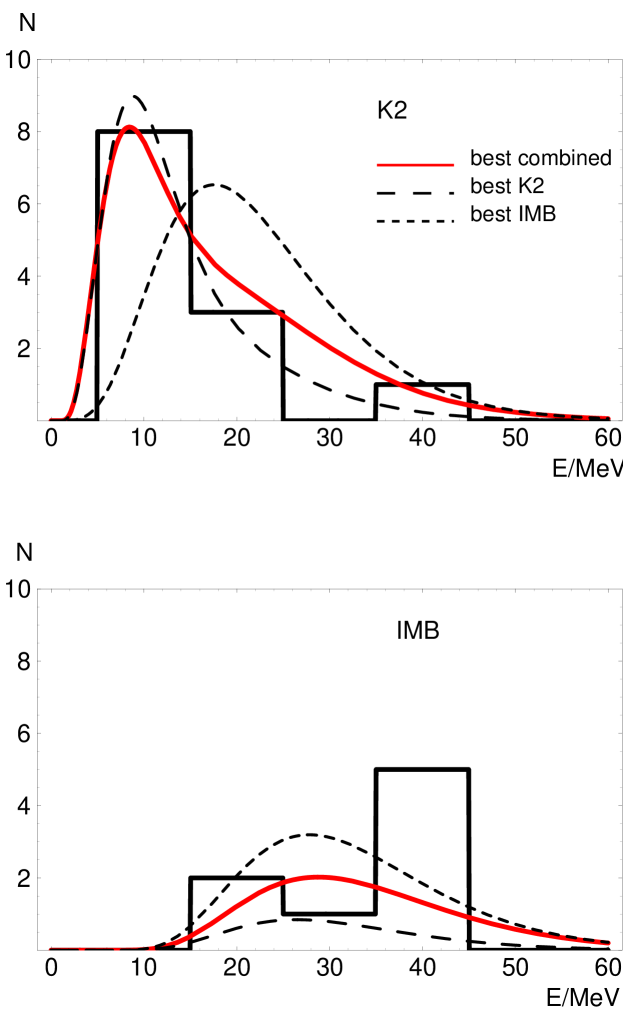
Figure 2: The observed energy spectra of events at K2 and IMB, as in Fig. 1, compared with the predicted spectra in the points of minimum $\chi^{2}$ for K2 only, IMB only and combined K2 and IMB data sets. The values of the parameters in these points are given in Table 1.

3.3 Combined analysis: results

Comparing the neutrino spectra favored by K2 and by IMB separately, one infers that a good combined fit exists. The key to see this is to observe that the average energy favored by IMB is similar to that of the hard component of the spectrum favored by K2 (see Table 1). Moreover, a very soft spectral component would affect IMB only marginally, due to threshold effects, as was mentioned in Sec. 3.2. Thus, one expects that the combination of the two data sets will favor a composite soft+hard spectrum qualitatively similar to that favored by the K2 data. The closeness to the K2-only result is motivated also by the fact that the K2 data dominate the statistics.

Some features of the $\chi^{2}_{87}$ function can be predicted as well. One expects degeneracies, even though not as extended as in the case of K2 and IMB separately. In particular, a degeneracy in $\chi^{2}_{87}$ should exists between the region with $E_{0\bar{e}}<E_{0x}$ and that with $E_{0\bar{e}}>E_{0x}$. The reason lies in the fact that, if the neutrino conversion is only partial (probability $0<P_{\bar{x}\bar{e}}<1$), the neutrino spectrum at Earth is symmetric under the transformation $P_{{\bar{e}}{\bar{e}}}{d}N_{\bar{e}}(E^{\prime})/{d}E^{\prime}\leftrightarrow(1-P_{{\bar{e}}{\bar{e}}}){d}N_{\bar{x}}(E^{\prime})/{d}E^{\prime}$ (see Eq. (3)). Such symmetry implies an approximate symmetry (broken by effects of oscillations in the Earth and by the energy dependence of $P_{{\bar{e}}{\bar{e}}}$) between the $E_{0\bar{e}}<E_{0x}$ and $E_{0\bar{e}}<E_{0x}$ portions of the parameter space.

The likelihood analysis, summarized in Table 1 and Figs. 2 and 3, confirms the intuitions. The predicted degeneracy is observed. The $\chi^{2}_{87}$ has two minima in the points $(\log(\sin^{2}\theta_{13}),E_{0\bar{e}},E_{0x},L_{\bar{e}},L_{x})=(-7,4.6~{}{\rm MeV},12.7~{}{\rm MeV},3.4\cdot 10^{53}~{}{\rm ergs},0.51\cdot 10^{53}~{}{\rm ergs})$ ($\chi^{2}_{87}=84.1$) and $(\log(\sin^{2}\theta_{13}),E_{0\bar{e}},E_{0x},L_{\bar{e}},L_{x})=(-3.6,12.5~{}{\rm MeV},5.2~{}{\rm MeV},6\cdot 10^{53}~{}{\rm ergs},1.7\cdot 10^{53}~{}{\rm ergs})$ ($\chi^{2}_{87}=84.7$). They correspond to the type of spectrum preferred by K2. Here, the same considerations done for the K2-only fit apply regards the conflict between the best fit scenario and theory. It is important to stress, however, that the $\chi^{2}_{87}$ function is very shallow, with many points having essentially the same goodness of fit as the minimum. The allowed region in the parameter space is very extended and includes theoretically motivated scenarios at 68% C.L. (Fig. 3). The region is compatible with the constraints on the neutrino spectrum put by light element synthesis during galactic chemical evolution [58, 59] (see also the related works [60, 61]), which favor rather soft muon and tau neutrino spectra: $E_{0x}\sim 15-18$ MeV [58]. A detailed comparison of those constraints with the results of this paper is not possible, however, due to the different working assumptions used here.

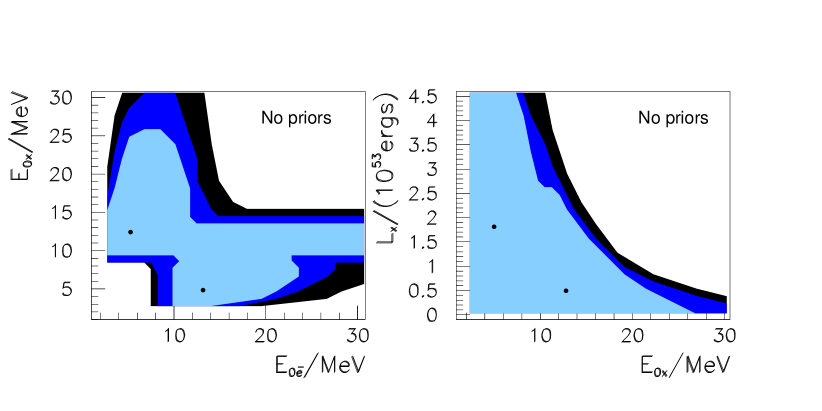
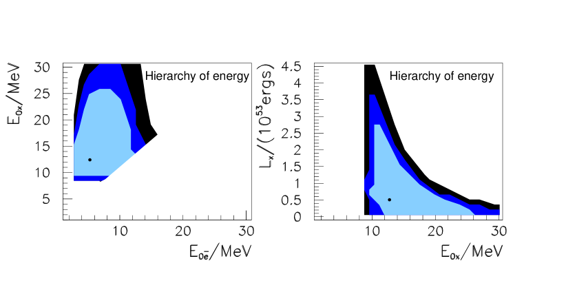
Figure 3: Projections of the 68%,90%,99% C.L. regions allowed by the SN1987A data on the planes $E_{0\bar{e}}-E_{0x}$ and $E_{0x}-L_{x}$, without any prior (upper panels) and with the hierarchy $E_{0\bar{e}}<E_{0x}$ (lower panels). The dots in each panel mark the projections of the points of maximum likelihood (see Table 1). The entire plane $E_{0\bar{e}}-L_{\bar{e}}$ (not shown) is allowed at 68% C.L..

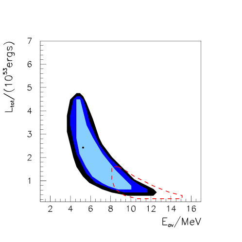
Figure 4: The best fit point and the regions allowed by the SN1987A data at 68%,90%,99% C.L. in the space of the average energy and luminosity of the $\mathrel{{\bar{\nu}}_{e}}$ flux at Earth (after conversion in the star). For comparison, I show the 99% C.L. region found in ref. [56] (dashed contour). There the same flux was described by a spectrum of the form (2).

The upper panels of Fig. 3 illustrate the details of the allowed region. There I give the projections on the $E_{0\bar{e}}-E_{0x}$ and $E_{0x}-L_{x}$ planes of the 5D allowed regions given by Eq. (6) for different confidence levels, together with the projections of the points of maximum likelihood. The figure confirms that a rather large portion of the parameter space is allowed, with better sensitivity to the $\mathrel{{\nu_{x}}}$ flux with respect to the $\mathrel{{\bar{\nu}}_{e}}$ one. Unless assumptions are made on the oscillation pattern, the $\mathrel{{\bar{\nu}}_{e}}$ flux is unconstrained, due to the possibility that the mass hierarchy be inverted with perfectly adiabatic conversion ($\sin^{2}\theta\mathrel{\vbox{\hbox{$>$}\nointerlineskip\hbox{$\sim$}}}few\cdot 10^{-4}$) inside the star. Under such conditions the original $\mathrel{{\bar{\nu}}_{e}}$ flux is completely converted into $\mathrel{{\nu_{x}}}$ and does not affect the observed $\mathrel{{\bar{\nu}}_{e}}$ signal. The $\mathrel{{\nu_{x}}}$ flux is constrained loosely: every value of $E_{0x}$ gives a good fit provided that the other parameters are suitably adjusted, and a similar statement is valid for $L_{x}$. Notice that the $\mathrel{{\nu_{x}}}$ luminosity and average energy are not constrained from below: indeed, they are allowed to be zero, in the case when the $\mathrel{{\bar{\nu}}_{e}}$ spectrum alone gives a good fit to the data. This can happen for all conversion patterns except the one with complete $\mathrel{{\bar{\nu}}_{e}}-\mathrel{{\nu_{x}}}$ permutation, and requires $E_{0\bar{e}}\sim 13-15$ MeV. In all cases, the region with $E_{0\bar{e}}\mathrel{\vbox{\hbox{$<$}\nointerlineskip\hbox{$\sim$}}}5$ MeV and $E_{0x}\mathrel{\vbox{\hbox{$<$}\nointerlineskip\hbox{$\sim$}}}5$ MeV is excluded because it gives a very soft neutrino spectrum, with a too small (or even vanishing) number of events at IMB.

If the analysis is restricted to the region motivated by the theory, $E_{0\bar{e}}<E_{0x}$ (lower panels of Fig. 3), some conclusions change: $E_{0x}$ must be larger than $\sim 10$ MeV and $E_{0\bar{e}}$ can not exceed $\sim 16$ MeV.

The Table 1 gives further details on one of the best fit points, confirming that it reproduces the data well in the number of events, $N_{K2}$ and $N_{IMB}$ and average energies, $\langle E\rangle_{K2}$ and $\langle E\rangle_{IMB}$. The goodness of the fit also appears from the superposition of the best fit spectrum with the data, in Fig. 2.

It is informative to present the results in a complementary way: by using a smaller number of variables and choosing parameters that describe the $\mathrel{{\bar{\nu}}_{e}}$ flux at Earth, instead than at the production point. Here I choose the average energy and luminosity of such flux, $E_{av}$ and $L_{tot}$. Fig. 4 shows the allowed region in the space of $E_{av}$ and $L_{tot}$, obtained after marginalizing the likelihood function over the three parameters orthogonal to these. For comparison, in the figure I also show an example of result obtained by fitting the data with two parameters only (i.e., keeping the other three parameters fixed instead than marginalizing over them). The example is taken from ref. [56] (fig. 2 there), where the $\mathrel{{\bar{\nu}}_{e}}$ flux at Earth is described by a spectrum of the form (2). The marginalized region confirms the finding of a particularly soft and luminous $\mathrel{{\bar{\nu}}_{e}}$ flux being favored by the data. The region is compatible with but more extended than the two-parameters result from ref. [56]. This reflects the fact that a five-variables parameterization includes neutrino spectra that fit the data well but are not reproduced with a smaller number of parameters. It is confirmed, therefore, that five-dimemsional and the two-dimensional methods are not equivalent.

4 The supernova rate

The cosmic rate of supernovae, $R_{SN}(z)$, can be inferred from astrophysical data in a variety of ways. Here I review two:

1. Measurements of the SNR  from observations of core collapse supernovae. This is the most direct method. To date, four measurements of the SNR have been made in this way, covering the interval of redshift $z\sim 0-0.9$ [14, 15, 16]. They are summarized in Table 2 and in Fig. 6. While the connection between the observations and the SNR is immediate, in principle, one should keep in mind that the results are affected by dust obscuration (extinction) and possible misidentification of the observed objects. These effects can be modeled theoretically and subtracted. Three of the measurements in Table 2 have been corrected in this way. The point at $z=0.26$, indicated with an empty circle in Fig. 6, is not corrected for extinction and for this reason it will not be included in the analysis here.

2. measurements of the star formation rate (SFR), $R_{SF}(z)$. From these, the SNR is found through the equation:

   $$R_{SN}(z) \simeq \frac{\int_{8M_{\odot}}^{50M_{\odot}}dm~{}\phi(m)}{\int_{0}^{125M_{\odot}}dm~{}m\phi(m)}R_{SF}(z)~{}\sim 10^{-2}M^{-1}_{\odot}R_{SF}(z)~{},$$ (7)

   (see e.g. [30]) where $\phi(m)$ is the initial mass function, decreasing roughly as a power $-2$ of the mass $m$, and $M_{\odot}$ is the mass of the Sun, $M_{\odot}\simeq 1.99\cdot 10^{30}$ Kg. The limits of integration represent the interval of mass for which a star becomes a core collapse supernova. With respect to direct searches of supernovae, this method has the advantage of higher statistics, since several measurements of the SFR are available, extending up to $z\sim 6-7$ (see e.g. [17, 18, 19] and [62] for an overview and further references). On the other hand, the SNR obtained with this approach is indirect: it is affected by a number of theoretical uncertainties through the relation (7), such as those on the initial mass function and on the interval of progenitor masses. The lower mass cut in (7) influences the normalization of the SNR  strongly. I refer to [62] for an in-depth discussion of these aspects. On top of the uncertainties mentioned, the SFR measurements are affected by extinction, like the direct supernova observations. Likely, the largest theoretical error is associated to the normalization of the SNR, however the possibility that the ratio of SFR and SNR be redshift-dependent – thus violating Eq. (7)– is not excluded. This is a possible source of error as well.

Clearly, the two methods are complementary. Their results agree in the basic facts: the SNR today is of order $R_{SN}(0)\sim 10^{-4}~{}{\rm yr^{-1}Mpc^{-3}}$. The rate increases with $z$ and is consistent with a broken power law:

$${R}_{{SN}}(z) = {R}_{{SN}}(0)(1+z)^{\beta}\quad{\rm for}\quad z<1$$ (8)

$$= {R}_{SN}(0)2^{\beta-\alpha}\,(1+z)^{\alpha}\quad{\rm for}\quad z>1~{}.$$

The values of ${R}_{{SN}}(0)$ favoured by the two approaches are somehow different, with method (2) giving a rate larger by a factor of $\sim 2-3$ with respect to method (1). This is probably a manifestation of the uncertainties that affect both methods. For example, it was checked that the discrepancy disappears if the lower mass cut in (7) is increased to $10M_{\odot}$ [62].

In this work I use method (1), motivated by its being direct and therefore more robust, and suitable for a conservative estimate of the DSN$\nu$F. For this specific application, its being limited to small resdhift is of little consequence, since the DSN$\nu$F above realistic energy thresholds is dominated by supernovae closer than $z\sim 1$ [30]. For this reason, here I fix $\alpha=0$, a value favored by the SFR data [62]. I perform a maximum likelihood analysis of the three extinction-corrected measurements of the SNR given in Table 2, to find the allowed region of the parameters $R_{SN}(0)$ and $\beta$ of Eq. (8). In the approximation of gaussian errors, I calculate the likelihood function ${\mathcal{L}}_{SNR}(R_{SN}(0),\beta)$ and $\chi^{2}_{SNR}\equiv-2\ln{\mathcal{L}_{SNR}}$.

reference	redshift $z$	$R_{SN}/(10^{-4}~{}{\rm yr^{-1}Mpc^{-3}})$
[14]	0	$0.59\pm 0.24$
[16]	0.26	$1.82^{+0.69}_{-0.56}$
[15]	0.3 (average)	$2.51^{+0.88}_{-0.75}$
[15]	0.7 (average)	$3.96^{+1.03}_{-1.06}$

Table 2: The measured supernova rate at different redshifts. The errors represent the $68\%$ confidence level intervals. The values of the redshift in the third and fourth row are averages over bins of redshift. The point at $z=0.26$ is not corrected for exctinction, while the other three points are.

The results are shown in figs. 5 and 6. The likelihood is maximal in the point $R_{SN}(0)=0.67\cdot 10^{-4}~{}{\rm yr^{-1}Mpc^{-3}}$, $\beta=3.44$, where the value of $\chi^{2}_{SNR}$ is $\chi^{2}_{SNR,min}=3.59$. Fig. 5 shows the point of maximum likelihood and the contours defined by $\chi^{2}_{SNR}-\chi^{2}_{SNR,min}=2.3,4.61,6.17$, corresponding to 68.3, 90, 95.4% confidence level (C.L.) . The results of the likelihood analysis confirm that the fit of the data with a power law curve is satisfactory. The allowed region is rather extended, with $R_{SN}(0)$ and $\beta$ varying by a factor of six and three respectively. In Fig. 6 the SNR functions allowed at given confidence level (shaded bands) and the best fit function are compared with the input measurements of Table 2. The figure also gives the SNR function found in ref. [62] using method (2), with the modified Salpeter B initial mass function (Table 2 in [62]) and the interval of progenitor masses as in Eq. (7). Confirming what already mentioned above, this curve has very similar logarithmic slope, $\beta=3.35$, but normalization higher by a factor of $\sim 2$ with respect to the best fit function found in this work.

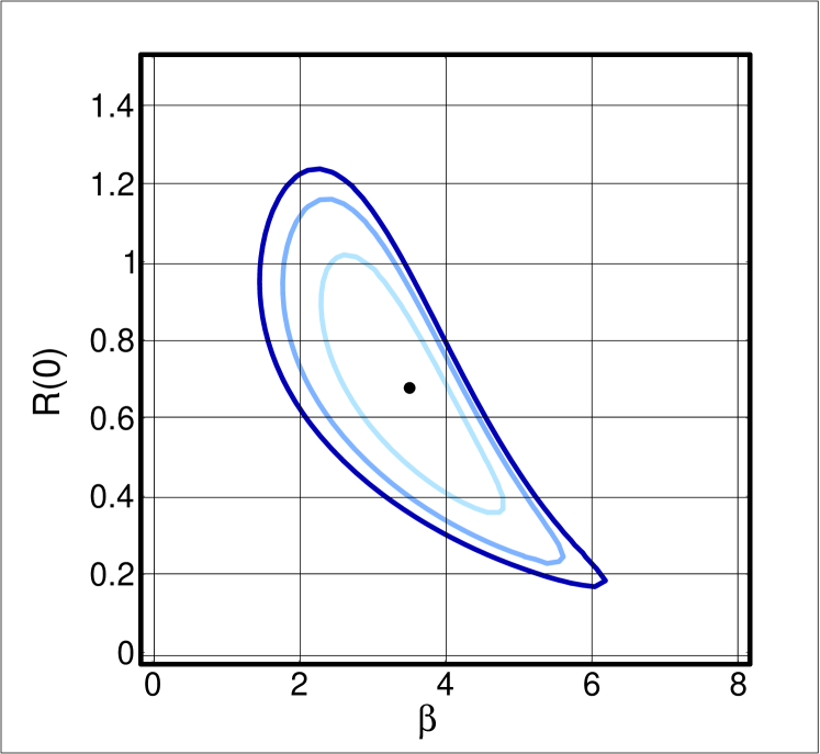
Figure 5: Best fit point and isocontours of $\chi^{2}$ in the space of the parameters describing the SNR function, $R_{SN}(z)$. These are the intercept, $R_{SN}(0)$ (in units of $10^{-4}~{}{\rm yr^{-1}~{}Mpc^{-3}}$) and the power, $\beta$. The contours refer to 68.3, 90, 95.4% C.L..

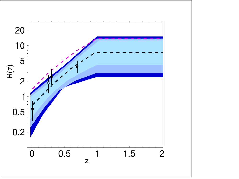
Figure 6: The SNR  (in units of $10^{-4}~{}{\rm yr^{-1}~{}Mpc^{-3}}$) as a function of the redshift, $z$. The colored (shaded) bands are the families of curves having parameters within the 68.3, 90, 95.4% C.L. contours of Fig. 5. The lower dashed line refers to the best fit parameters of my analysis. The measurements of the SNR, with $1~{}\sigma$ error bar, are shown (from Table 2). Of these, the point marked with an empty circle was not included in the analysis because it is not corrected for exctinction. The upper dashed line results from using, instead than core collapse data, the SFR data with a specific initial mass function (from ref. [62], see text).

In connection to this, one may consider performing a global analysis of the direct SNR measurements and of the SFR data together. Such analysis warrants a separate work, necessary to make the different data sets compatible with each other; this in turn requires, among other things, a careful study of the connection between SNR and SFR, and an evaluation of the different methods used by different authors in their statistical analyses and in the correction for dust obscuration. This has not been done so far and represents the next step with respect to this paper. In consideration of the uncertainties on the normalization of the SFR, I expect that the combination with the SFR data would improve the constraint on $\beta$, with only little improvement on $R_{SN}(0)$.

Studies have indicated that the $z=0$ measurement used here may underestimate the local SNR by a factor of two or so [63, 2]. In absence of a new determination of the local rate, one can only give examples of how the likelihood results would change if the $z=0$ point was higher. If I rescale this point and its error by a factor of two (three) the new point of maximum likelihood is $R_{SN}(0)=1.26\cdot 10^{-4}~{}{\rm yr^{-1}Mpc^{-3}}$, $\beta=2.21$ ($R_{SN}(0)=1.72\cdot 10^{-4}~{}{\rm yr^{-1}Mpc^{-3}}$, $\beta=1.55$), with only minor change in the value of $\chi^{2}_{SNR,min}$. As will be shown, the effect of a higher $R_{SN}(0)$ is partially compensated by that of a smaller $\beta$, so that the impact of this change on the DSN$\nu$F is only of tens of per cent.

5 Diffuse neutrino flux

5.1 The calculation

In the framework adopted here, the DSN$\nu$F depends on seven parameters: five describing the neutrino flux (two average energies, two luminosities and one mixing angle) and two describing the SNR (the rate at $z=0$ and the power, $\beta$). To calculate the diffuse flux and the uncertainty on it, it is necessary to combine the information from both the SN1987A and the SNR  data sets consistently.

I perform this combination as follows:

• I obtain the total likelihood of the neutrino and SNR data together, ${\mathcal{L}}_{tot}$. Since the two sets of data are uncorrelated, this is done by simply multiplying the two individual likelihoods. The combined $\chi^{2}$ is the sum of the two pieces: $\chi^{2}=\chi^{2}_{87}+\chi^{2}_{SNR}$.

• Using Eq. (4) I compute the likelihood for the $\mathrel{{\bar{\nu}}_{e}}$ diffuse flux in a detector, $\Phi$, by marginalizing ${\mathcal{L}}_{tot}$ with respect to all the six quantities orthogonal to $\Phi$. If the likelihood function is close to a gaussian near its maximum, for a given $\Phi$ the marginalized $\chi^{2}$ – called $\chi^{2}_{\Phi}$ from here on – is well approximated by the global $\chi^{2}$ minimized with respect to the other six variables. Here I adopt this approximation, widely used in data analysis literature (see [64] for an example).

• I use $\chi^{2}_{\Phi}$ to find the best value of $\Phi$, defined as the one that minimizes $\chi^{2}_{\Phi}$, and the 99% C.L. interval for it, defined by the difference $\chi^{2}_{\Phi}-\chi^{2}_{\Phi,min}=6.65$.

Results are given for three cuts in the neutrino energy: $E>19.3,11.3,5.3$ MeV. The first corresponds to the threshold applied in the search of the DSN$\nu$F at SK [6], while the second represents a potential improvement that SK could achieve with the proposed Gadolinium addition [65]. The last cut, $E>5.3$ MeV, is the technical limit given by the photomultipliers distribution in the SK tank and would apply only in the – currently unfeasible – case of complete background subtraction. It should be stressed that with such low threshold the DSN$\nu$F starts to have a non-negligible contribution (about $\sim 50\%$ [30]) from supernovae at $z>1$, and thus it depends on the value of the power $\alpha$ in Eq. (8). Here I used $\alpha=0$, therefore the results of this work for the lowest threshold have indicative character only; they could change by several tens of per cent for different values of $\alpha$.

The effects of neutrino flavor conversion inside the star are included. I calculated the effects of oscillations inside the Earth, using a realistic matter density profile [66], and in the assumption of isotropic DSN$\nu$F. I find that these oscillations affect the DSN$\nu$F by less than $\sim 10\%$, and therefore I neglect them for simplicity.

The same procedure of marginalization discussed for the flux can be done for the number of events in a detector. Here I do the calculation for SK and the inverse beta decay events: $\mathrel{{\bar{\nu}}_{e}}+p\rightarrow n+e^{+}$. This is by far the dominant signal in water, which justifies neglecting other reactions. I took the fiducial volume of SK of 22.5 kilotons and detection efficiency of $\simeq 93\%$ above $\sim 7$ MeV [3, 51]. In reality, the efficiency depends on the specific experimental cuts. In the case of the published SK analysis the efficiency is 47% (79%) below (above) 34 MeV [67]. Thus, considering the exponential decay of the flux with the energy, the rates given here would have to be rescaled down by roughly a factor of 2 to be applicable to the current SK setup.

5.2 Results

The results for the flux and numbers of events are presented in Table 3 and Fig. 7.

For the current SK threshold of $19.3$ MeV, the $\mathrel{{\bar{\nu}}_{e}}$ flux in a detector is of the order of $\sim 10^{-1}~{}{\rm cm^{-2}s^{-1}}$. The value of maximum likelihood is $\Phi=0.15~{}{\rm cm^{-2}s^{-1}}$ and is obtained with the parameters that minimize both $\chi^{2}_{87}$ and $\chi^{2}_{SNR}$, Secs. 3 and 4. With 99% C.L., the flux must be larger than $\sim 0.05~{}{\rm cm^{-2}s^{-1}}$ and can not exceed $0.35~{}{\rm cm^{-2}s^{-1}}$, almost a factor of 4 below the SK limit. The event rate is below 0.7 events/year. The width of the 99% interval is about a factor of 7-8 both in the flux and event rate.

The flux increases by almost one order of magnitude if the threshold is lowered to 11.3 MeV. This is explained by the exponential decay of the flux with energy. The event rate instead increases more moderately with the lowering of the threshold. This is because the detection cross section is proportional to the square of the energy, $\sigma\propto E^{2}$, and therefore the spectrum of the observed positrons decays less rapidly than the neutrino spectrum. From Table 3 it appears that for threshold at 11.3 MeV or lower the goal of one event/year is possible, but not guaranteed.

To expect at least one event/year with 99% C.L. a larger detector than SK is necessary. A volume of water 2.5 times the volume of SK would be sufficient for the lowest threshold of 5.3 MeV, while with the current SK threshold a detector $\sim 10$ times larger is required. This may become a reality with the next generation Megaton detectors. With a fiducial volume 20 times larger than SK, these detectors would register $\sim 2-14$ events/year for the higher threshold, with a maximum of $\sim 44$ events/year with detection above 5.3 MeV.

	$E>19.3~{}{\rm MeV}$	$E>11.3~{}{\rm MeV}$	$E>5.3~{}{\rm MeV}$
	$\Phi/({\rm cm^{-2}s^{-1}})$	$\Phi/({\rm cm^{-2}s^{-1}})$	$\Phi/({\rm cm^{-2}s^{-1}})$
	$\left[N/{\rm yr^{-1}}\right]$	$\left[N/{\rm yr^{-1}}\right]$	$\left[N/{\rm yr^{-1}}\right]$
best	0.15	0.93	9.4
	$\left[0.28\right]$	$\left[0.73\right]$	$\left[1.1\right]$
68% C.L.	0.12 - 0.21	0.64 - 1.19	6.4 - 13.5
	$\left[0.19-0.41\right]$	$\left[0.51-0.85\right]$	$\left[0.77-1.43\right]$
90% C.L.	0.08 - 0.27	0.50 - 1.39	4.9 - 16.7
	$\left[0.14-0.52\right]$	$\left[0.40-1.23\right]$	$\left[0.62-1.72\right]$
99% C.L.	0.05 - 0.35	0.33 - 2.1	3.2 - 22.6
	$\left[0.09-0.7\right]$	$\left[0.27-1.6\right]$	$\left[0.43-2.2\right]$

Table 3: The predicted flux of $\mathrel{{\bar{\nu}}_{e}}$ in a detector in the point of maximum likelihood and in the intervals of 68, 90, 99% C.L. for different energy thresholds. The numbers in brackets have the same meaning, but for the rates of $\mathrel{{\bar{\nu}}_{e}}+p\rightarrow n+e^{+}$ events at SuperKamiokande for $\sim 93\%$ detection efficiency (see text).

What is the contribution of the individual sources of error to the total uncertainty on the DSN$\nu$For event rate? Fig. 7 answers this question for the event rate. For the three thresholds, the figure shows the error bars obtained by marginalizing the likelihood over a subset of parameters while keeping the others fixed at their best fit values. It appears that the error bar from the SNR (with fixed neutrino parameters) is smaller than the one due to the neutrino spectra (e.g. fixed SNR). The first is about a factor of 3 wide, while for the second the width is a factor of 4-7 depending on the threshold. Notice that this width is larger for higher threshold, reflecting the larger uncertainty in the high energy tail of the SN1987A data with respect to their full spectrum.

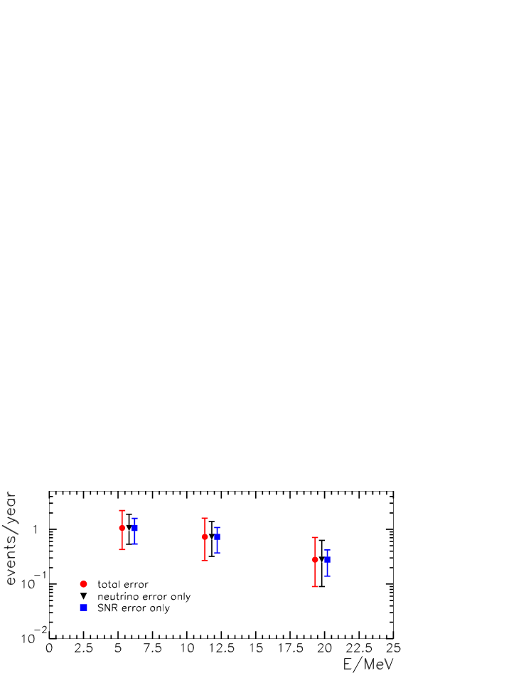
Figure 7: The number of $\mathrel{{\bar{\nu}}_{e}}+p\rightarrow n+e^{+}$ events per year at SuperKamiokande as a function of the energy threshold $E_{th}$ (horizontal axis). Results are given for $E_{th}=5.3,11.3,19.3$ MeV in neutrino energy. For each of these, three cases are shown (shifted in energy for visual convenience): (i) total error, from the marginalization of the likelihood function in the whole parameter space, (ii) error from the neutrino spectrum only, obtained by marginalization with the supernova rate function fixed at its best fit point, (iii) error from the supernova rate only, obtained by keeping the neutrino parameters fixed at the best fit values. The markers give the values in the best fit point, while the bars represent the 99% C.L. interval (“error”).

Let me now discuss the validity of the results and possible generalizations. A relevant question is how the interval of values of the DSN$\nu$F depends on the details of the analysis of the SN1987A data, and, in particular, on possible priors on the neutrino parameters. I checked that the results have little dependence on those. For example, the interval for the flux above 19.3 MeV (see Table 3) is unchanged if I impose (simultaneously) the constraints: $10~{}{\rm MeV}<E_{0\bar{e}}<20~{}{\rm MeV}$, $E_{0\bar{e}}<E_{x}$ and $0.5<L_{\bar{e}}/L_{x}<2$. This is explained with the parameter space being largely degenerate, so that a restricted portion of it still covers almost all the physically different possibilities. For the same reasons the results are also practically insensitive to different parameterizations of the original fluxes (e.g., different $\alpha_{\bar{e}}$ and/or $\alpha_{x}$).

The analysis here does not include systematic errors. Still, here I briefly discuss how the prediction of the DSN$\nu$F would change if some of the inputs turned out to be systematically wrong and were corrected. Let us consider the event in which $R_{SN}(0)$ is higher than what used here (see discussion in Sec. 4). With $R_{SN}(0)$ increased by a factor of two (three) the maximum likelihood value of the flux is $\Phi=0.20~{}{\rm cm^{-2}s^{-1}}$ ($\Phi=0.23~{}{\rm cm^{-2}s^{-1}}$) above the current SK threshold of $19.3$ MeV. This is at most a $\sim 50\%$ increase with respect to the result in Table 3. Another example refers to the poorly known normalization of the SNR. Specifically, my results could become a factor of two higher if it is confirmed that normalization of the SNR is two times higher as favored by the SFR measurements (Sec. 4 and Fig. 6). A combined fit of the supernova data and SFR measurements would reduce the uncertainty on the slope $\beta$ and therefore the total error on the DSN$\nu$F. To check how this error would change, I performed the same calculation outlined in this section with $\beta$ fixed at its best fit value, $\beta=3.44$, which happens to be nearly the same both in the SNR  and in the SFR data analyses (Sec. 4). I find that the results for the DSN$\nu$F do not change appreciably, due to the large degeneracies between different sets of parameters.

Besides technical details, it has to be stressed that the results given here are valid if the SN1987A neutrino flux is typical and thus represents a generic output of a core collapse supernova. This question will be answered by data from a future galactic supernova. At the moment, recent calculations show that the main observational features of SN1987A are reproduced by the standard neutrino-driven explosion mechanism, disfavoring possible anomalies in the SN1987A event [68].

6 Discussion and conclusions

Let me summarize this work. I have calculated the $\mathrel{{\bar{\nu}}_{e}}$ component of the DSN$\nu$F in a detector, using the information on the neutrino spectra from SN1987A and the information on the supernova rate from direct observations of core collapse supernovae. I calculated the likelihood functions for the SN1987A data and for the supernova rate measurements, and marginalized the combined likelihood to find the interval of DSN$\nu$F allowed at a given confidence level.

The SN1987A data favor a composite neutrino spectrum, meaning that a scenario with inverted mass hierarchy and $\sin^{2}\theta_{13}\mathrel{\vbox{\hbox{$>$}\nointerlineskip\hbox{$\sim$}}}10^{-4}$ is disfavored (in agreement with refs. [52, 53]). The best fit spectrum reproduces both the K2 and IMB data well, even if IMB alone favors a thermal spectrum over a composite one. It is characterized by a very soft and very luminous component, with parameters in contrast with general theoretical arguments and with numerical simulations. The allowed region of the parameter space, however, is very extended and includes more natural scenarios at 68% C.L..

The supernova rate measurements allow a present rate of about $(0.2-1.2)\cdot 10^{-4}~{}{\rm Mpc^{-3}~{}yr^{-1}}$ and a power of increase with $z$ of about 2 - 6 . Also in this case a large region of parameters is allowed. The function that best fits the data has similar power, $\beta\sim 3$, but different normalization (about a factor of two smaller) with respect to what is inferred using data on the star formation rate and the proportionality of this rate to the supernova rate.

The results for the DSN$\nu$F ($\mathrel{{\bar{\nu}}_{e}}$ component) show that the flux above the current SK threshold is likely to be about one order of magnitude below the current upper limit of $1.2~{}{\rm cm^{-2}s^{-1}}$, and is smaller than this limit by a factor of $\sim 4$ with 99% confidence. This factor of 4 is the minimal improvement that SK should achieve if the energy threshold remains the same. Any lowering of the threshold would significantly enhance the possibility to detect the DSN$\nu$F. Still, however, if my prediction is correct, a Megaton detector would be necessary to expect a detection with very high confidence.

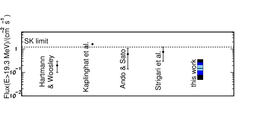
Figure 8: The results of different authors (from left to right: refs. [25], [26] (upper bound only), [31, 30], [29] and this work) for the flux of $\mathrel{{\bar{\nu}}_{e}}$ above a threshold of 19.3 MeV (in neutrino energy). For this work the colored (shaded) bands correspond to 68%, 90% and 99% confidence levels, with the central like marking the maximum likelihood value. The SK limit is shown as well (dashed line).

How does this work compare to others in the field? Fig. 8 answers this question, by presenting the results of different papers [25, 26, 31, 30, 29] for the $\mathrel{{\bar{\nu}}_{e}}$ diffuse flux above $19.3$ MeV, with the interval of uncertainty associated to it. The authors quoted in the figure are only a small sample of all those that have calculated the DSN$\nu$F; they were chosen for illustration purpose and because their results can be directly compared to each other’s and to mine. Each of them used neutrino spectra from a number of numerical simulations, and inferred the supernova rate from the star formation rate. They also gave a tentative uncertainty on their result, associated with the lack of consensus on numerical codes and with the error on the star formation rate. The error bars in the figure, as well as the central points, do not have a statistical meaning except for the result of this paper, where the shaded areas represent the intervals allowed at 68%, 90% and 99% C.L. and the central line marks the maximum likelihood value.

From the figure it appears that the interval of flux calculated here overlaps with the prediction of other authors within the error, but extends to lower values. In particular, it is the only calculation which allows a flux smaller than $\sim 0.1~{}{\rm cm^{-2}s^{-1}}$. The differences between my results and the larger flux – close to the SK limit – allowed by Strigari et al. [29] and by Ando and Sato [31, 30], are due to the different inputs used by these authors: a factor of about two higher SNR (see discussion in Sec. 4) and larger neutrino flux at high energy, due to the harder neutrino spectra used, with $E_{0x}$ up to $\sim 24$ MeV. These spectra are motivated by numerical calculations of neutrino transport, but are known to be at best marginally compatible with the SN1987A data [51, 53, 54], a fact that this paper confirms. Hartmann and Woosley [25] used a supernova rate function similar to that of Strigari et al. and of Ando and Sato, together with softer neutrino spectrum: a thermal spectrum with temperature of $\sim$ 4 MeV. This explains their finding a lower flux with respect to other authors. The result by Kaplinghat et al. [26] is a conservative upper bound obtained with a unoscillated neutrino spectrum and the maximum SNR compatible with metal enrichment history.

The comparison with the previous literature shows that this work is complementary to others. It is especially useful because it gives an idea of how the predicted DSN$\nu$F can change with a change of the method of calculation or of the inputs. This should be encouraging to work to improve our knowledge of the inputs, in particular of the neutrino spectra and of the normalization of the SNR. This paper also makes the point that the flux may be smaller than generally expected, thus supporting the case for a next generation of neutrino detectors with larger volumes and/or lower energy thresholds.

References

- [1] N. Arnaud et al., Astropart. Phys. 21, 201 (2004).
- [2] S. Ando, J. F. Beacom and H. Yuksel, Phys. Rev. Lett. 95, 171101 (2005).
- [3] K. Hirata et al., Phys. Rev. Lett. 58, 1490 (1987).
- [4] K. S. Hirata et al., Phys. Rev. D38, 448 (1988).
- [5] R. M. Bionta et al., Phys. Rev. Lett. 58, 1494 (1987).
- [6] M. Malek et al., Phys. Rev. Lett. 90, 061101 (2003).
- [7] K. Eguchi et al., Phys. Rev. Lett. 92, 071301 (2004).
- [8] W. C. Haxton and C. W. Johnson, Nature 333, 325 (1988).
- [9] J. N. Bahcall, Nature 333, 301 (1988).
- [10] C. K. Jung (1999), hep-ex/0005046.
- [11] R. J. Wilkes (2005), hep-ex/0507097.
- [12] K. Nakamura, Int. J. Mod. Phys. A18, 4053 (2003).
- [13] L. Mosca, Nucl. Phys. Proc. Suppl. 138, 203 (2005).
- [14] E. Cappellaro et al., Astron. and Astrophys. 351, 459 (1999).
- [15] T. Dahlen et al., Astrophys. J. 613, 189 (2004).
- [16] E. Cappellaro et al., Astron. and Astrophys. 430, 83 (2005).
- [17] S. Cole et al., Mon. Not. Roy. Astron. Soc. 326, 255 (2001).
- [18] K. Glazebrook et al., Astrophys. J. 587, 55 (2003).
- [19] I. K. Baldry and K. Glazebrook, Astrophys. J. 593, 258 (2003).
- [20] D. Schiminovich et al., Astrophys. J. 619, L47 (2005).
- [21] L. E. Strigari, et al., JCAP 0504, 017 (2005).
- [22] M. Fukugita and M. Kawasaki, Mon. Not. Roy. Astron. Soc. 340, L7 (2003).
- [23] T. Totani, K. Sato and Y. Yoshii, Astrophys. J. 460, 303 (1996).
- [24] R. A. Malaney, Astropart. Phys. 7, 125 (1997).
- [25] D. H. Hartmann and S. E. Woosley, Astropart. Phys. 7, 137 (1997).
- [26] M. Kaplinghat, G. Steigman, and T. P. Walker, Phys. Rev. D62, 043001 (2000).
- [27] S. Ando, K. Sato and T. Totani, Astropart. Phys. 18 (2003) 307.
- [28] S. Ando and K. Sato, Phys. Lett. B559, 113 (2003).
- [29] L. E. Strigari, M. Kaplinghat, G. Steigman, and T. P. Walker, JCAP 0403, 007 (2004).
- [30] S. Ando and K. Sato, New J. Phys. 6, 170 (2004).
- [31] S. Ando, Astrophys. J. 607, 20 (2004).
- [32] A. G. Cocco, A. Ereditato, G. Fiorillo, G. Mangano and V. Pettorino, JCAP 0412, 002 (2004).
- [33] J. F. Beacom and L. E. Strigari, hep-ph/0508202.
- [34] M. T. Keil, G. G. Raffelt, and H.-T. Janka, Astrophys. J. 590, 971 (2003).
- [35] A. S. Dighe and A. Y. Smirnov, Phys. Rev. D62, 033007 (2000).
- [36] S. P. Mikheev and A. Y. Smirnov, Sov. Phys. JETP 64 (1986) 4 [Zh. Eksp. Teor. Fiz. 91 (1986) 7].
- [37] P. I. Krastev and S. T. Petcov, Phys. Lett. B205, 84 (1988).
- [38] C. Lunardini and A. Y. Smirnov, JCAP 0306, 009 (2003).
- [39] C. Lunardini and A. Y. Smirnov, Nucl. Phys. B616, 307 (2001.
- [40] L. Hernquist and V. Springel, Mon. Not. Roy. Astron. Soc. 341, 1253 (2003).
- [41] T. A. Thompson, A. Burrows, and P. A. Pinto, Astrophys. J. 592, 434, (2003).
- [42] R. C. Mitchell et al., Astrophys. J., 574, 293, 2002
- [43] C. Lunardini and A. Y. Smirnov, Astropart. Phys. 21, 703, (2004).
- [44] B. Aharmim et al.,(2005), nucl-ex/0502021.
- [45] T. Araki et al., Phys. Rev. Lett. 94, 081801 (2005).
- [46] Y. Fukuda et al., Phys. Rev. Lett. 81, 1562 (1998).
- [47] Y. Ashie et al., Phys. Rev. Lett. 93, 101801 (2004).
- [48] E. Aliu et al., Phys. Rev. Lett. 94, 081802 (2005).
- [49] R. C. Schirato, G. M. Fuller, (2002), astro-ph/0205390.
- [50] A. Strumia and F. Vissani, Phys. Lett. B 564, 42 (2003).
- [51] B. Jegerlehner, F. Neubig, and G. Raffelt, Phys. Rev. D54, 1194 (1996).
- [52] C. Lunardini and A. Y. Smirnov, Phys. Rev. D63, 073009 (2001.
- [53] H. Minakata and H. Nunokawa, Phys. Lett. B504, 301 (2001).
- [54] M. Kachelriess, R. Tomas and J. W. F. Valle, JHEP 0101, 030 (2001).
- [55] V. Barger, D. Marfatia and B. P. Wood, Phys. Lett. B 532, 19 (2002).
- [56] A. Mirizzi and G. G. Raffelt, astro-ph/0508612.
- [57] J. M. LoSecco, Phys. Rev. D 39, 1013 (1989).
- [58] T. Yoshida, T. Kajino and D. H. Hartmann, Phys. Rev. Lett. 94, 231101 (2005).
- [59] T. Yoshida, T. Kajino, H. Yokomakura, K. Kimura, A. Takamura and D. H. Hartmann, astro-ph/0602195.
- [60] S. E. Woosley and W. C. Haxton, Nature 334, 45 (1988).
- [61] W. C. Haxton, arXiv:nucl-th/9712049.
- [62] A. M. Hopkins and J. F. Beacom, astro-ph/0601463.
- [63] F. Mannucci et al., Astron. Astrophys. 401, 519 (2003).
- [64] M. Maltoni, T. Schwetz, M. A. Tortola and J. W. F. Valle, New J. Phys. 6, 122 (2004)
- [65] J. F. Beacom and M. R. Vagins, Phys. Rev. Lett. 93, 171101 (2004).
- [66] A. M. Dziewonski and S. T. Anderson, Phys. Earth Planet Interiors 25, 297 (1981).
- [67] M. S. Malek, PhD Thesis, State University of New York at Stony Brook, Aug. 2003, available at http://www-sk.icrr.u-tokyo.ac.jp/sk/pub/.
- [68] K. Kifonidis, T. Plewa, L. Scheck, H. T. Janka and E. Mueller, astro-ph/0511369.