Cosmology with Weak Lensing Surveys

Abstract

Weak lensing - Cosmology: methods - Statistical Weak gravitational lensing is responsible for the shearing and magnification of the images of high-redshift sources due to the presence of intervening mass. Since the lensing effects arise from deflections of the light rays due to fluctuations of the gravitational potential, they can be directly related to the underlying density field of the large-scale structures. Weak gravitational surveys are complimentary to both galaxy surveys and cosmic microwave background observations as they probe unbiased non-linear matter power spectra at medium redshift. Ongoing CMB experiments such as WMAP and future Planck satellite mission will measure the standard cosmological parameters with unprecedented accuracy. The focus of attention will then shift to understanding the nature of dark matter and vacuum energy: several recent studies suggest that lensing is the best method for constraining the dark energy equation of state. During the next 5 year period ongoing and future weak lensing surveys such as the Joint Dark Energy Mission (JDEM, e.g. SNAP) or the Large-aperture Synoptic Survey Telescope (LSST) will play a major role in advancing our understanding of the universe in this direction. In this review article we describe various aspects of probing the matter power spectrum and the bispectrum and other related statistics with weak lensing surveys. This can be used to probe the background dynamics of the universe as well as the nature of dark matter and dark energy.

1 Introduction

Gravitational lensing refers to the deflection of light from distant sources by the gravitational force arising from massive bodies present along the line of sight. Such an effect was already raised by Newton in 1704. Indeed, as derived in textbooks on Newtonian mechanics a particle starting at velocity $v$ at large distance from a spherical body of mass $M$ is deflected by an angle $\alpha_{N}=2GM/rv^{2}$, where $r$ is the impact parameter and we assumed that $\alpha_{N}$ is small. Setting $v=c$ one obtains the “Newtonian” value for the deflection of light, as calculated by Cavendish around 1784. As is well known, General Relativity yields twice the Newtonian value, $\alpha_{GR}=2\alpha_{N}$, as obtained by Einstein (1915). The agreement of this prediction with the deflection of light from distant stars by the sun measured during the solar eclipse of 1919 (Dyson, Eddington & Davidson 1920) was a great success for Einstein’s theory and brought General Relativity to the general attention (the eclipse allows one to detect stars with a line of sight which comes close to the sun).

In a similar fashion, light rays emitted by a distant galaxy are deflected by the matter distribution along the line of sight toward the observer. This creates a distortion of the image of this galaxy, which is both sheared and amplified (or attenuated). While the gravitational lensing effect due to a rare massive object like a cluster of galaxies can be very strong and lead to multiple images, the distortion associated with typical density fluctuations is rather modest (of the order of $1\%$). Besides, galaxies are not exactly spherical. Therefore, one needs to average over many galaxies and cross-correlate their observed ellipticity in order to extract a meaningfull signal and this field of investigation is called “statistical weak gravitational lensing”. Thus, the aim of “weak lensing surveys” is to obtain the images of distant galaxies over a whole region on the sky in order to estimate the coherent shear over large angular scales due to the large scale structures of the universe. This allows us to derive information on the structure and dynamics of the universe from the statistical deformation of the images of distant galaxies (for more detailed reviews or articles see for instance Miralda-Escude 1991, Bartelmann & Schneider 2001, Mellier 1999, Refregier 2003).

In the last few years many studies have managed to detect cosmological shear in random patches of the sky (Bacon, Refregier & Ellis 2000; Bacon et al. 2003; Brown et al. 2003; Hamana et al. 2003; Hämmerle et al. 2002; Hoekstra, Yee & Gladders 2002a; Hoekstra et al. 2002a; Jarvis et al. 2002; Kaiser, Wilson & Luppino 2000; Maoli et al. 2001; Refregier, Rhodes & Groth 2002; Rhodes, Refregier & Groth 2001; van Waerbeke et al. 2000; van Waerbeke et al. 2001a; van Waerbeke et al. 2002; Wittman et al. 2000). While early studies were primarily concerned with the detection of a non-zero weak lensing signal, present weak lensing studies are already putting constraints on cosmological parameters such as the matter density parameter $\Omega_{m}$ and the normalisation $\sigma_{8}$ of the power-spectrum of matter density fluctuations. These works also help to break parameter degeneracies when used along with other cosmological probes such as Cosmic Microwave Background (CMBR) observations. In combination with galaxy redshift surveys they can be used to study the bias associated with various galaxies which will be useful for galaxy formation scenarios thereby providing much needed clues to the galaxy formation processes. In this article we review the recent progress that has been made and various prospects of future weak lensing surveys.

2 Using weak gravitational lensing effects for cosmology

2.1 Theory

Until very recently most of the information about the power spectrum of cosmological density perturbations was obtained from large scale galaxy surveys and Cosmic Microwave Background Radiation observations. However, galaxy surveys only probe the clustering of luminous matter while CMBR observations measure the power spectrum at a very early linear stage. Weak lensing studies fill in the gap by giving us a direct handle on the cosmological power spectrum at a medium redshift in an unbiased way, from linear to non-linear scales. As recalled in the introduction, light rays emitted by a distant object are deflected because of the inhomogeneites of the matter distribution along the line of sight. This implies that a source located at the angular position ${\bf\theta}$ on the sky is actually observed at the angular location ${\bf\theta}+\delta{\bf\theta}$ given by the symmetric shear matrix (Schneider, Ehlers & Falco 1992; Jain, Seljak & White 2000):

$$\psi_{ij}=\frac{\partial\delta\theta_{i}}{\partial\theta_{j}}=\left(\begin{array}[]{cc}\kappa+\gamma_{1}&\gamma_{2}\\ \gamma_{2}&\kappa-\gamma_{1}\end{array}\right)=2\int_{0}^{\chi_{s}}{\rm d}\chi\frac{{\cal D}(\chi){\cal D}(\chi_{s}-\chi)}{{\cal D}(\chi_{s})}\partial_{i}\partial_{j}\phi(\chi),$$ (1)

where we assumed distortions are small. Here $\chi$ is the radial comoving distance, ${\cal D}$ is the angular distance and the subscript $s$ refers to the source redshift, while $\phi$ is the perturbed gravitational potential (i.e. the source term to Poisson’s equation is the perturbed density $\rho-{\overline{\rho}}$ where ${\overline{\rho}}$ is the mean density of the universe). Thus, eq.(1) clearly shows how the deflection angles $\delta{\bf\theta}$ are related to the matter distribution along the line of sight. Of course, in practice we cannot measure the deflections $\delta{\bf\theta}$ themselves (since usually we do not know the actual positions ${\bf\theta}$) but we can measure the distortions $\psi_{ij}$ (assuming we know the shape of the source). Thus, the convergence $\kappa$ describes isotropic distortions of images (contractions or dilatations) while the shear ${\bf\gamma}=(\gamma_{1},\gamma_{2})$ describes anisotropic distortions. Since galaxies are not spherical we need to average the observed ellipticities of many galaxies over a given region on the sky to obtain the coherent weak lensing shear over this area (or its low order moments) associated with large scale structures.

2.2 From galaxy ellipticities to weak lensing shear

In order to measure the shear $(\gamma_{1},\gamma_{2})$ from the shape of galaxies one usually computes the second moments $I_{ij}$ of the galaxy surface brightness which can be combined to yield its observed ellipticity ${\bf e}_{\rm obs}$ (Kaiser, Squires & Broadhurst 1995):

$$I_{ij}=\int{\rm d}^{2}\theta\;\;\theta_{i}\theta_{j}I({\bf\theta})W({\bf\theta}),\hskip 14.22636pt{\bf e}_{\rm obs}=\left(\frac{I_{11}-I_{22}}{I_{11}+I_{22}},\frac{2I_{12}}{I_{11}+I_{22}}\right).$$ (2)

The window function $W({\bf\theta})$ is centered on the galaxy and suppresses the noise from other parts of the sky. If there were no observational errors the observed ellipticity ${\bf e}_{\rm obs}$ would be related to the actual galaxy ellipticity by ${\bf e}$ by: ${\bf e}_{\rm obs}={\bf e}+{\bf\gamma}$ in the linear regime (small lensing distortions). Then, assuming that galaxy ellipticities are uncorrelated over large distances we can recover the coherent weak lensing shear ${\bf\gamma}$ by summing over many sources. Note that in doing so we must also take into account the redshift distribution of the galaxies.

In practice, we must first remove the observational noise from ${\bf e}_{\rm obs}$. Since weak lensing distortions are only of the order of a few percents the various stages of data reduction need to be performed with extreme care. First, it is desirable to have a homogeneous depth over the field and as small a seeing as possible. Besides, it is advantageous to have a wide survey which contains many uncorrelated cells (since we wish to perform a statistical analysis). Next, after flat fielding (to remove sensitivity differences between pixels) one maps the images from “detector coordinates” to actual astronomical coordinates taking into account telescope distortion (for instance by using a set of reference stars and modeling the detector distortion by a low-order polynomial). Then, one needs to correct for the asymmetry and smearing of the point-spread function (PSF), which describes the response of the imaging system to an object consisting of a perfect point. This distortion may be due to atmospheric turbulence, guiding errors and telescope optics. This can be corrected by measuring the shape of the stars present in the field of view, which ought to be spherical and can act as point sources for this purpose. Note that in general the PSF can vary with time and needs to be modeled individually for each image. See Kaiser et al. (1999) for a detailed description of image processing.

Elaborate methods have been developed to tackle these issues. The most commonly used technique of Kaiser, Squires & Broadhurst (KSB, 1995) is based on the measurement of the quadrupole moment of the galaxy surface brightness (see eq.(2)) and it treats the PSF convolution analytically to first order. It was later generalised by several authors (Luppino & Kaiser 1997; Hoekstra et al. 1998). Recent studies have thoroughly tested KSB techniques and found them to be sufficient for present surveys (e.g. Erben et al. 1991 and Bacon et al. 2001). However, a higher level of accuracy will be needed for future generations of surveys. Many improvements and alternatives were studied in the recent past to deal with these issues by modifying or extending KSB (Kaiser 2000; Rhodes, Refregier & Groth 2000), fitting observed galaxy shapes with analytical models (Kuijken 1999) or decomposing galaxy shapes over orthogonal basis functions (Bernstein & Jarvis 2002; Refregier & Bacon 2003).

Note that weak lensing effects can also be measured through the induced magnification associated with the convergence $\kappa$. This changes the flux received from a distant source, its observed size and the number counts of objects.

2.3 Numerical simulations

Figure 1: Left panel: The blue elongated disks represent observed images of background galaxies. The dark matter filaments from numerical simulations which were used to simulate the survey are also plotted to show alignemnets of ellipticites of observed galaxies with underlying filamentary structures (Figure courtesy: Stephane Colombi). Right panel: Simulated shear field (short solid lines) and convergence field (background intensity) are shown (Figure courtesy: Patrick Simon) .

Once the data analysis has allowed one to obtain a shear map from a weak lensing survey, one can use it to put constraints on cosmology by comparing the observational data with predictions associated with different cosmological models. On large scales where the density contrast is small ($|\delta|\ll 1$ with $\delta=(\rho-{\overline{\rho}})/{\overline{\rho}}$ where ${\overline{\rho}}$ is the mean density of the universe) one can use an analytical perturbative approach to obtain the properties of weak lensing (Bernardeau, van Waerbeke & Mellier 1997). However, at small non-linear scales there is no rigorous analytical method to derive the statistics of the density contrast $\delta$. Therefore, one needs to use numerical simulations to make the contact between observations and the relevant cosmological parameters which describe the universe. To do so, one first builds a numerical simulation of the growth of large scale structures in the universe through gravitational instability for a given set of cosmological parameters. This gives a map of the density contrast and of the gravitational potential along a line of sight up to high redshift (one actually piles up several simulation boxes up to the source redshift). Then, one can follow the propagation of light through the simulation boxes (ray tracing technique, Blandford et al. 1991; Jain, Seljak & White 2000; Premadi et al. 2001; Wambsganss, Cen & Ostriker 1998) or integrate the shear matrix along the line of sight (Barber et al. 2000; Hamana, Martel & Futamase 2000). Finally, by averaging over many lines of sight one can obtain the statistical properties of weak lensing effects for a given set of cosmological parameters. By performing many simulations for a whole range of cosmologies and comparing their results with observations one can constrain these cosmological parameters. In practice, in order to break degeneracies between various parameters one combines weak lensing surveys with other cosmological probes (CMBR observations, cluster statistics, etc.) to obtain best constraints. Note that such a procedure assumes that the actual universe belongs to the class of models described by these cosmological parameters. In particular, one usually assumes a “cold-dark matter” (CDM) scenario (most of the matter is in the form of an unknown cold and collisionless component, which is necessary to explain many astronomical observations like the rotation curves of spiral galaxies) where non-linear objects (like galaxies) and large scale structures (filaments, voids,etc.) build up through the amplification by gravitational instability of small initial Gaussian density fluctuations, while the whole universe follows a “big-bang” dynamics described by the Friedmann-Robertson-Walker metric (Peebles 1993). The agreement of many observational tests with the predictions derived from such scenarios strongly suggests this global picture is indeed correct (until we find a discrepancy which cannot be reconciled) and observational measurements can be further used to obtain the values of cosmological parameters like the mean matter density in the universe.

3 Weak lensing statistics

3.1 Power spectrum

From eq.(1) we can see that the means $\langle\kappa\rangle$ and $\langle{\bf\gamma}\rangle$ vanish (since $\langle\delta\rangle=0$ whence $\langle\phi\rangle=0$). Therefore, the lowest-order statistics we can measure are second-order moments like $\langle\kappa^{2}\rangle$. In particular, the power spectrum $P_{\kappa}(s)$ of the weak lensing convergence, defined in two-dimensional Fourier space by $\langle\kappa({\bf s})\kappa({\bf s^{\prime}})^{*}\rangle=\delta_{D}({\bf s}-{\bf s^{\prime}})P_{\kappa}(s)$, is related to the power spectrum $P_{3D}$ of the three-dimensional density contrast $\delta$, by (Kaiser 1998):

$$P_{\kappa}(s)=\frac{9\Omega_{m}^{2}}{4}\frac{H_{0}^{4}}{c^{4}}\int_{0}^{\infty}\frac{{\rm d}\chi}{a^{2}}\;P_{3D}\left(\frac{s}{{\cal D}};z\right)\left[\int_{z}^{\infty}{\rm d}z_{s}\;n(z_{s})\frac{{\cal D}(\chi_{s}-\chi)}{{\cal D}(\chi_{s})}\right]^{2}.$$ (3)

Here we used the small-angle approximation. The notations are the same as in eq.(1), the redshift $z$ corresponds to the radial distance $\chi$ while $n(z_{s})$ is the galaxy redshift distribution normalized to unity. We noted $c$ the speed of light, $H_{0}$ the present value of the Hubble constant and $\Omega_{m}$ the matter density parameter. From eq.(1) one can check that the power spectrum of the shear ${\bf\gamma}$ is equal to $P_{\kappa}(s)$ (thus $\langle\kappa^{2}\rangle=\langle|{\bf\gamma}|^{2}\rangle$). In practice, one does not measure the power spectrum $P_{\kappa}(s)$ itself but the variance of the shear smoothed with a suitable filter. Thus, one can consider the smoothed convergence, shear components and the aperture mass $M_{\rm ap}$ (Schneider et al. 1998a) defined by:

$$\kappa_{s}=\int{\rm d}^{2}\theta\;U({\bf\theta})\kappa({\bf\theta}),\;\;\gamma_{is}=\int{\rm d}^{2}\theta\;U({\bf\theta})\gamma_{i}({\bf\theta}),\;\;M_{\rm ap}=\int{\rm d}^{2}\theta\;Q({\bf\theta})\gamma_{t}({\bf\theta}),$$ (4)

where $U({\bf\theta})$ is a top-hat of size $\theta_{s}$ while $Q({\bf\theta})$ is a compensated filter (of zero mean) and $\gamma_{t}$ is the tangential shear (with respect to the window center). The advantage of the compensated quantity $M_{\rm ap}$ is that it provides a pass-band filter which directly probes the convergence power at wavenumber $s\sim 1/\theta_{s}$. Indeed, since the filter $Q({\bf\theta})$ has a zero mean (i.e. $\int{\rm d}^{2}\theta\;Q({\bf\theta})=0$) the contribution from wavelengths much larger than $\theta_{s}$ is suppressed, which is not the case for the observables $\kappa_{s}$ and $\gamma_{is}$ defined with the top-hat filter $U$. The drawback is that the variance $\langle M_{\rm ap}^{2}\rangle$ is smaller than $\langle\kappa_{s}^{2}\rangle=2\langle\gamma_{is}^{2}\rangle$. Another property of the aperture mass $M_{\rm ap}$ is that it can be expressed both in terms of the shear, as in eq.(4), or in terms of the convergence $\kappa$ (Schneider 1996). Of course, the variance of all these observables can be written in terms of the power spectrum $P_{\kappa}(s)$.

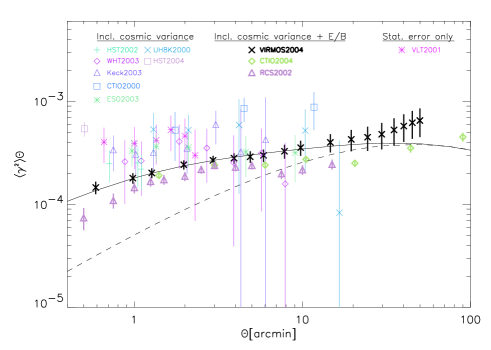
Figure 2: A compilation of results from various surveys. The figure shows $\langle|\gamma|^{2}\rangle$ times the radius of the smoothing scale $\theta$ as a function of smoothing angular scale. The solid line is the best fit model, and the dashed line shows the linear prediction ($\Omega_{m}=0.3$, $\Omega_{\Lambda}=0.7$, $\sigma_{8}=0.83$ and source redshift $z_{s}=0.9$). The three thick symbols show the observations where an Electric/Magnetic mode separation was carried out, the thin symbols show measurements without such separation. It is interesting to see that all measurements with no separation predict a larger $\sigma_{8}$. The RCS and CTIO2004 survey results are from low redshift ($z_{s}=0.6$) shallow surveys. These measurements were rescaled in order to have an equivalent source redshift of $z_{s}=0.9$ (to match others). Figure courtesy Ludovic Van Waerbeke.

Then, one could divide the survey area on the sky into numerous patches of radius $\theta_{s}$ and perform the average of $M_{\rm ap}^{2}$ (for instance) over all cells. However, this method is not well suited to real weak lensing surveys which have a complex geometry with many holes of various sizes, as one needs to remove the areas contaminated by bright stars or observational defects. This makes it impracticable to draw a circular filter across the data. Hence, one usually defines shear two-point correlations, such as $\xi_{t}=\langle\gamma_{t}\gamma_{t}\rangle$ and $\xi_{r}=\langle\gamma_{r}\gamma_{r}\rangle$ from the tangential and radial components $\gamma_{t}$ and $\gamma_{r}$ of the shear (the cross-correlation $\langle\gamma_{t}\gamma_{r}\rangle$ vanishes by symmetry), see Schneider, van Waerbeke & Mellier (2002). These two-point correlations are measured by summing the shear products over all galaxy pairs separated by some angle ${\bf\theta}$. This bypasses the problem raised by the numerous holes present in the survey. Next, the variance of the shear or of the aperture mass can be expressed as integrals over $\xi_{t}$ and $\xi_{r}$ (Crittenden et al. 2002; Schneider, van Waerbeke & Mellier 2002). Alternatively, one can study the shear two-point correlations themselves.

As in electromagnetism, the tensor field ${\bf\gamma}$ can be decomposed into an electric ($E$ mode, i.e. gradient) component and a magnetic ($B$ mode, i.e. curl) component. However, since weak lensing effects are produced by a scalar field (the gravitational potential $\phi$) the $B$ mode is zero. Therefore, any detection of the $B$ mode in the data signals the presence of systematics or other effects not related to weak lensing like intrinsic galaxy alignements. It can be shown that the aperture mass $M_{\rm ap}$ given in eq.(4) only selects the $E$ mode, while the same quantity measured after all galaxies have been rotated by 45 degrees (noted for instance $M_{\times}$) selects the $B$ mode (Crittenden et al. 2002; Schneider, van Waerbeke & Mellier 2002). Therefore, by computing the variances $\langle M_{\rm ap}^{2}\rangle$ and $\langle M_{\times}^{2}\rangle$ one can estimate the amount of contamination to the weak lensing signal. Although present surveys find a non-zero $B$ mode it is sufficiently smaller than the $E$ mode to support the detection of a real weak lensing signal due to large scale structures. Unfortunately, it is not clear how the $B$ mode can be substracted from the $E$ mode to improve the accuracy of the measurements. This remains an important issue for weak lensing surveys.

By varying the smoothing angle $\theta_{s}$ or the pair separation $\theta$ one can constrain the shape of the convergence power spectrum $P_{\kappa}(s)$ and of the underlying matter power spectrum $P_{3D}(k)$ over the range probed by the survey, as measured by the usual parameter $\Gamma$. On the other hand, as can be seen in eq.(3) the amplitude of the weak lensing signal measures a combination of the matter density parameter $\Omega_{m}$ and of the normalization of the matter power spectrum $P_{3D}$ (usually noted $\sigma_{8}$). The dependence on other cosmological parameters is much smaller but one must pay attention to the rather strong dependence on the redshift of the sources.

After early failed searches for weak lensing signals which include studies mainly using photometric plates (Kristian 1967; Valdes, Jarvis & Tyson 1983), a first attempt with CCD (Mould et al. 1994) only derived an upper limit. However Villumsen (1995) using the same data reported a detection, and a few years later Schneider et al. (1998b) reported detection of weak lensing. Nevertheless, the sky coverage of these studies was probably too small. After the initial discovery within a short period of time four groups independently confirmed detection of cosmic shear in random patches of the sky (Bacon, Refregier & Ellis 2000; Kaiser, Wilson & Luppino 2000; van Waerbeke et al. 2000; Witman et al. 2000). It is interesting to note that all of these initial observations were done using 4m-class telescope. Since then there has been an explosion of shear measurements coming from various observational teams from ground based observations (Bacon et al. 2003; Brown et al. 2003; Hamana et al. 2003; Hoekstra et al. 2002; Hoekstra, Yee & Gladders 2002; Jarvis et al. 2002; Maoli et al. 2001; van Waerbeke et al. 2001a; van Waerbeke et al. 2002) as well as from space using the Hubble Space Telescope (see e.g. Hämmerle et al. 2002; Rhodes, Refregier & Groth 2001). Figure 2 shows a compilation of present results from various surveys. Although there is a clear detection and the various experiments agree with the theoretical expectations, there is still a some dispersion between different surveys. In particular, it appears that the separation between $E$ modes and $B$ modes needs to be considered with care.

A more ambitious goal than measuring a few cosmological parameters like $(\Omega_{m},\sigma_{8},\Gamma)$ is to use weak lensing surveys to reconstruct the matter power spectrum $P_{3D}$ itself, by inverting eq.(3). This is not an easy task because the integration along the line of sight implies that a whole range of physical three dimensional wavenumbers $k$ contribute to a given two dimensional wavenumber $s$. Another problem is that the evolution with redshift $z$ of the matter power spectrum $P_{3D}(k;z)$ in eq.(3) only factorizes as $P_{3D}(k;z)=D_{+}(z)P_{L}(k)$ in the linear regime (which in principles allows one to recover the function of one variable $P_{L}(k)$ from $P_{\kappa}(s)$). In the non-linear regime this factorization is no longer valid and one needs to work with the function of two variables $P_{3D}(k;z)$. In practice one may circumvent this problem by using a mapping from the linear prediction $D_{+}(z)P_{L}(k)$ onto the non-linear power spectrum (or by neglecting the departures from linear growth) but this procedure introduces some modeling associated with this mapping (or some approximation). Alternatively, one may restrict the reconstruction to very large linear scales. An estimate of the two dimensional converge power spectrum was obtained in Pen et al. (2002) and Brown et al. (2003) while Pen et al. (2003a) derived the three dimensional matter density power spectrum.

3.2 Non-Gaussianities

To break the degeneracy between the parameters $\Omega_{m}$ and $\sigma_{8}$ present in two-point statistics one can combine weak lensing observations with other cosmological probes (like CMBR) or consider higher order moments of weak lensing observables. Indeed, even if the initial conditions are Gaussian, since the dynamics is non-linear (this is an unstable self-gravitating expanding system) non-Gaussianities develop and in the non-linear regime the density field becomes strongly non-Gaussian. This can be seen from the constraints $\langle\delta\rangle=0$ and $\delta\geq-1$ (because the matter density $\rho$ is positive) which implie that in the highly non-linear regime ($\langle\delta^{2}\rangle\gg 1$) the probability distribution of the density contrast $\delta$ must be far from Gaussian. In the quasi-linear regime where a perturbative approach is valid (with Gaussian initial conditions) one can show that the skewness $S_{3}=\langle\kappa_{s}^{3}\rangle/\langle\kappa_{s}^{2}\rangle^{2}$ is independent of the density power spectrum normalization $\sigma_{8}$ (the same property is valid for other observables like $M_{\rm ap}$ which are linear over the matter density field). Therefore, by measuring the second and third order moments of the convergence or of the aperture mass at large angular scales one can obtain a constraint on $\Omega_{m}$ (Bernardeau, van Waerbeke & Mellier 1997). Alternatively, from the skewness of weak lensing observables one can derive the skewness of the matter density field in the linear regime and check that the scenario of the growth of large scale structures through gravitational instability from initial Gaussian conditions is valid.

Again, because of the numerous holes within the survey area one first computes shear three-point correlations (called the bispectrum in Fourier space) by summing over galaxy triplets and next writes $\langle M_{\rm ap}^{3}\rangle$ as an integral over these three-point correlations. Applying this method to the Virmos-Descart data Pen et al. (2003b) were able to detect $S_{3}$ and to infer an upper bound $\Omega_{m}<0.5$ by comparison with simulations. Alternatively, one can study the shear three-point correlation itself, averaged over some angular scale. This can be optimised by identifying typical shear patterns (such as the flow of the shear vector ${\bf\gamma}$ around a galaxy pair) in order to select the three point product which yields the larger signal (recall that $\gamma$ has two components which offers many choices). Bernardeau et al. (2002) obtained in this fashion the first detection of non-Gaussianity in a weak lensing survey. Next, one could measure higher order moments of weak lensing observables. Note that for the shear components odd order moments vanish by symmetry so that one needs to consider the fourth-order moment to go beyond the variance (Takada & Jain 2002). However, higher order moments are increasingly noisy (Valageas, Munshi & Barber 2005) so that it has not been possible to go beyond the skewness yet.

In practice, most of the angular range probed by weak lensing surveys is actually in the transition domain from the linear to highly non-linear regimes (from $10^{\prime}$ down to $1^{\prime}$). Therefore, it is important to have a reliable prediction for these mildly and highly non-linear scales, once the cosmology and the initial conditions are specified. Since there is no rigorous analytical framework to investigate this regime numerical simulations play a key role to obtain the non-linear evolution of the matter power spectrum and of higher order statistics (Peacock & Dodds 1996; Smith et al. 2003). Based on these simulation results it is possible to build analytical models which can describe the low order moments of weak lensing observables or their full probability distribution. This can be done through a hierarchical ansatz where all higher-order density correlations are expressed in terms of the two-point correlation (Barber, Munshi & Valageas 2004; Valageas, Munshi & Barber 2005). Then, the probability distribution of weak lensing observables can be directly written in terms of the probability distribution of the matter density. In some cases the mere existence of this relationship allows one to discriminate between analytical models for the density field which are very similar (Munshi, Valageas & Barber 2004). Alternatively, one can use a halo model where the matter distribution is described as a collection of halos (Cooray & Sheth 2002) and the low order moments of weak lensing observables can be derived by averaging over the statistics of these halos (Takada & Jain 2003a,b). On the other hand, one can use weak lensing to constrain halo properties and to detect substructures (Dolney, Jain & Takada 2004).

3.3 Weak lensing probe of astrophysics at small scales

Since weak lensing surveys directly probe the matter distribution in the universe, they can be used together with galaxy surveys to estimate the bias of galaxies and the matter-galaxy cross-correlation. Present generation surveys are already proving useful in this direction (Simon et al. 2004). Future weak lensing surveys will have a direct impact on galaxy formation scenarios by probing the bias associated with various galaxy types and its evolution with redshift $z_{s}$.

4 Problems to overcome

Weak lensing surveys are only beginning to address cosmological questions like the value of cosmological parameters. In order to exploit gravitational lensing effects for cosmological purposes with a good accurvay we still need to improve our control of various sources of errors. We list below a few of these issues.

Intrinsic galaxy alignment. Weak lensing measurements can be contaminated by a possible intrinsic alignment of galaxy ellipticites, which could be induced by tidal fields (see Heavens 2001). Theoretical estimates of such an effect have been performed using numerical (Jing 2002; Croft & Metzler 2000; Heavens, Refregier & Heymans 2000) and analytical techniques (Catalan, Kamionkowski & Blandford 20001; Crittenden et al. 2001, 2002; Lee & Pen 2001; Mackey, White & Kamionkowski 2002). Measurements of intrinsic ellipticity correlation of galaxies have also been attempted (Pen, Lee & Seljak 2000; Brown et al. 2002). At present there is no clear agreement among various analytical predictions regarding the amplitude of this effect, although one can safely expect that shallower surveys should be more affected than deeper surveys. To suppress this possible source of errors in future surveys one will use photometric redshifts to select galaxies which are separated in redshift space. However, in a recent study Hirata & Seljak (2004) have shown that even the galaxy intrinsic ellipticity and the shear field can be correlated which would make things further complicated.

Redshift distribution. Weak lensing effects depend on the source redshift which needs to be known with a good accuracy in order to obtain tight constraints on cosmology. This is a difficult task because of the depth of weak lensing surveys. Moreover, any dependence of the source redshift distribution on the direction on the sky could affect the comparison of observations with theory. Over the course of next few years, photometric redshift surveys (e.g. COMBO17 ) are going to be increasingly prevalent. On the other hand, if the survey has a broad source redshift distribution, background sources can be lensed by foreground galaxies or by matter density peaks correlated with foreground sources. This effect yields additional terms to the weak lensing signal which must be taken into account (Bernardeau 1998a; Hamana et al. 2002).

PSF correction. The most serious issue (for the observational part) is the distortion induced by the PSF. At present the KSB method allows an accuracy of a few percent. In order to reach higher precision one needs to develop more efficient techniques. Space telescopes avoid the atmospheric turbulence and show a more stable PSF but they still require a significant correction.

Non-linear evolution. Most of the angular scales measured by weak lensing surveys ($<10^{\prime}$) probe the non-linear regime of gravitational clustering. Since no analytical methods are available, one needs to use numerical simulations to obtain theoretical predictions which can be compared with weak lensing observations (van Waerbeke et al. 2001b). Current simulations only provide an accuracy of the order of $10\%$ for two-point statistics while higher order statistics are increasingly difficult to obtain. Recent works such as Smith et al. (2003) already show an improvement over previous estimates but the development of more powerful simulations remains necessary.

Numerical simulations. Simulation techniques also need to be generalised and improved upon to quantify the corrections due to many realistic details such as source-lens coupling, source clustering and redshift distribution. Contributions from the finite size of the surveys and intrinsic noise can be investigated in great details to optimise returns from future surveys. The construction of such mock catalogues will pave the way for analytical modelling of various realistic systematics.

5 Prospects

Although CMBR observations together with other probes like SNIa experiments and cluster statistics have already provided impressive information on some key cosmological issues, weak lensing surveys are a promising tool for cosmological purposes. First, used in combination with other observations like CMBR missions they can help break degeneracies between cosmological parameters and they can tighten the constraints on models. Second, they offer a unique method to probe the matter distribution on quasi-linear to non-linear scales which cannot be done by other techniques. We list below a few of the goals of future surveys.

Power spectrum reconstruction. Using the redshift position of the source together with the weak lensing signal itself one can study the evolution with redshift of the matter distribution. It may even be possible to map the three dimensional matter distribution (Hu & Keton 2002; Massey et al. 2004; Taylor 2001).

Cosmological parameters. The measured cosmic signals from small weak lensing surveys can be used to provide constraints on the cosmological parameters $\Omega_{m},\sigma_{8}$ and $\Gamma$ (the source redshift distribution also plays a very important role). A much bigger survey with much higher sky coverage allows to constrain many more cosmological parameters (Hu & Tegmark 1999), see also Tereno et al. (2005) for a recent joint analysis of weak lensing surveys with current WMAP-1 year and CBI data employing Monte Carlo Markov Chain calculation of a seven parameter model, which is more realistic than previously employed Fisher matrix based analysis. A principal component analysis which probes various parameter degeneracies is also presented. Next generation surveys will be independently able to probe such issues without having to assume a specific structure formation scenarios with a primordial power law spectrum. They will also constrain the evolution of the dark energy and test quintessence models (Benabed & van Waerbeke 2004; Hu & Jain 2004). In particular, lensing tomography (i.e. binning galaxy sources in redshift space) can prove useful to tighten the constraints on cosmology (Hu 1999; Takada & Jain 2004).

Primordial non-Gaussianities. Results from future surveys will also be very useful in constraining primordial non-Gaussianity predicted by some early universe theories. Generalised theories of gravity can have very different predictions regarding gravity induced non-Gaussianites as compared to GR, which can also be probed using future data. A joint analysis of power spectrum and bi-spectrum from weak lensing surveys thus will provide a very powerful way to constrain, not only cosmological parameters, but early universe theories and alternative theories of gravitation (see also Schmid, Uzan & Riazuelo 2005). Thus, in a recent work Bernardeau (2004) has studied the possibility of constraining higher-dimensional gravity from cosmic shear three-point correlation function.

Future surveys. The constraints on cosmology brought by weak lensing measurements will gradually improve as ongoing surveys are fully exploited, such as the CFHT (van Waerbeke, Mellier & Hoekstra 2005), the Deep Lens Survey (Wittmann et al. 2002), the SDSS (Sheldon et al. 2004). Accurate measures of cosmological parameters and tests of various cosmological scenarios will be possible with future missions, such as the CFHT Legacy Surveys (Tereno et al. 2005), the Visible and Infrared Survey Telescope for Astronomy or VISTA (Taylor et al. 2003), the Large aperture Synoptic Survey Telescope or LSST (Tyson et al. 2002a,b), novel Panoramic Survey Telescope and Rapid Response System or Pan-STARRS (Kaiser, Tonry & Luppino 2000), Supernova Acceleration Probe satellite or SNAP (Perlmutter et al. 2003) and Advanced Camera for Surveys (ACS) on HST. Ground based and space-based observations have a complimentary role to play in near future. While space based observations can provide a stable PSF and hence a reduced level of systematics ground based observations can survey a larger fraction of the sky. However, a high level of degeneracy among various lensing observables implies that only a small number of independent linear combinations of them can be extracted from future surveys. On the other hand, even smaller surveys will be very helpful in improving cosmological constraints when analysed jointly with external data-sets such as data from all-sky cosmic microwave background surveys (Hu & Tegmark 1999).

Weak lensing of background galaxy samples is limited only to a low source redshift($z_{s}\approx 2$). However as pointed out by various authors (e.g. Bernardeau 1997, 1998b; Cooray & Kesden 2003; Hirata & Seljak 2003; Seljak 1996; van Waerbeke, Bernardeau & Benabed 2000; Zaldarriaga & Seljak 1999) weak lensing of CMBR can be used to study the matter clustering all the way up to recombination era. It was also realised thanks to these studies that distinct non-Gaussian signal left due to lensing can actually be used to reconstruct the foreground mass distribution. With forthcoming high resolution CMB missions such as Planck Surveyor such a program will be made feasible.

Possibilities of weak lensing studies using radio surveys such as FIRST have also been studied (Kamionkowski et al. 1997; Refregier et al. 1998). Upcoming radio surveys such as Low Frequency Array or LOFAR and Square Kilometer Array (SKA) will provide unique opportunity in this direction (see e.g. Schneider 1999).

6 Conclusions

Next generation of cosmic shear surveys with MEGACAM at CFHT or VISTA at Paranal or even space based panoramic cameras will improve by order of magnitude in detail and precision. This will eventually lead to projected mass reconstruction, similar to APM galaxy surveys. By allowing measurement of higher order correlation functions thanks to huge sky coverage and low shot noise, it will break the degeneracy between cosmological parameters such as $\sigma_{8}$ and $\Omega_{m}$. Using priors from external data set such as recent all sky CMB experiments, weak lensing experiments can already put strong constraints on extended set of cosmological parameters such as the shape parameter $\Gamma$ of power spectrum or the primordial spectral slope $n_{s}$ and running of the spectral index. As surveys get bigger probing larger angular scales will be easier and as these scales are free from non-linearites they will be very useful to probe the background cosmological dynamics. With photometric redshifts it will also be possible to make 3D dark matter maps. On a longer timescales very large surveys will start probing scales larger than $10$ degrees which will eventually permit us to constraint $\Omega_{\Lambda}$ or any quintessence fields. While at large angular scale weak lensing measurements will increasingly focus on cosmological dynamics and nature of dark energy, small angular scale measurements will give us clues to the clustering of baryons relative to dark matter distributions. This will be possible by comparing weak lensing maps against galaxy surveys.

- [1]
- [2] Bacon D.J., Refregier A., Ellis R., 2000, MNRAS 318, 625
- [3] Bacon D.J., Refregier A., Clowe D., Ellis R., 2001, MNRAS 325, 1065
- [4] Bacon D.J., Massey R., Refregier A., Ellis R., 2003, MNRAS 344, 673
- [5] Barber A.J., Munshi D., Valageas P., 2004, MNRAS 347, 667
- [6] Barber A.J., Thomas P.A., Couchman H.M.P., Fluke C.J., 2000, MNRAS 319, 267
- [7] Bartelmann M., Schneider P., 2001, Phys.Rept. 340, 291
- [8] Benabed K., van Waerbeke L., 2004, Phys. Rev. D 70, 123515
- [9] Bernardeau F., 1997, Astron. Astrophys. 324, 15
- [10] Bernardeau F., 1998a, Astron. Astrophys. 338, 375
- [11] Bernardeau F., 1998b, Astron. Astrophys. 338, 375
- [12] Bernardeau F., 2005, submitted to PRL, astro-ph/0409224
- [13] Bernardeau F., van Waerbeke L., Mellier Y., 1997, Astron. Astrophys. 322, 1
- [14] Bernardeau F., Mellier Y., van Waerbeke L., 2002, Astron. Astrophys. 389, L28
- [15] Bernstein G.M., Jarvis M., 2002, A. J. 123, 583
- [16] Blandford R.D., Saust A.B., Brainerd T.G., Villumsen J.V., 1991, MNRAS 251, 600
- [17] Brown M.L., Taylor A.N., Hambly N.C., Dye S., 2002, MNRAS 333, 501
- [18] Brown M., Taylor A.N., Bacon D.J., Gray M.E., Dye S., Meisenheimer K., Wolf C., 2003, MNRAS 341, 100
- [19] Catalan P., Kamionkowksi M., Blandford R., 2001, MNRAS 320, 7
- [20] Cooray A., Kesden M., 2003, New Astron. 8, 231
- [21] Cooray A., Sheth R., 2002, Phys. Rept. 372, 1
- [22] Crittenden R., Natarajan P., Pen U.-L., Theuns T., 2001, Ap. J. 559, 552
- [23] Crittenden R., Natarajan P., Pen U.-L., Theuns T., 2002, Ap. J. 568, 20
- [24] Croft R.A.C., Metzler C.A., 2000, Ap. J. 545, 561
- [25] Dolney D., Jain B., Takada M., 2004, MNRAS 352, 1019
- [26] Dyson F.W., Eddington A.S., Davidson C., 1920, Phil. Trans. Roy. Soc. 220A, 291
- [27] Einstein A., 1915, Sitzungber. preuss. Akad. Wiss., 831
- [28] Erben T., van Waerbeke L., Bertin E., Mellier Y., Schneider P., 2001, Astron. Astrophys. 366, 717
- [29] Hamana T., Martel H., Futamase T., 2000, Ap. J. 529, 56
- [30] Hamana T., Colombi S., Thion A., Devriendt J., Mellier Y., Bernardeau F., 2002, MNRAS 330, 365
- [31] Hamana T., Miyazaki S., Shimasaku K., Furusawa H., Doi M., et al., 2003, Ap.J. 597, 98
- [32] Hämmerle H., Miralles J.M., Schneider P., Erben T., Fosbury R.A., 2002, Astron. Astrophys. 385, 743
- [33] Heavens A.F., 2001. Intrinsic Galaxy Alignments and Weak Gravitational Lensing, Yale Worksh. Shapes Galaxies Haloes, May. astro-ph/0109063
- [34] Heavens A., Refregier A., Heymans C., 2000, MNRAS 319, 649
- [35] Hirata C.M., Seljak U., 2003, Phys. Rev. D 67, 043001
- [36] Hirata C.M., Seljak U., 2004, Phys. Rev. D 70, 063526
- [37] Hoekstra H., Franx M., Kuijken K., Squires G., 1998, Ap. J. 504, 636
- [38] Hoekstra H., Yee H.K.C., Gladders M,. 2002, Ap. J. 577, 595
- [39] Hoekstra H., Yee H.K.C., Gladders M., Felipe Barrientos L., Hall P.B., Infante L., 2002, Ap. J. 572, 55
- [40] Hu W., 1999, Ap. J. 522, L21
- [41] Hu W., Tegmark M., 1999, Ap. J. 514, L65
- [42] Hu W., Keeton C.R., 2002, Phys. Rev. D 66, 063506
- [43] Hu W., Jain B., 2004, Phys. Rev. D 70, 043009
- [44] Jain B., Seljak U., White S.D.M., 2000, Ap. J. 530, 547
- [45] Jarvis M., Bernstein G.M., Fisher P., Smith D., Jain B., Tyson J.A., Wittman D., 2002,Ap. J. 125, 1014
- [46] Jing Y.P., 2002, MNRAS 335, L89
- [47] Kaiser N., 1998, Ap. J. 498, 26
- [48] Kaiser N., 2000, Ap. J. 537, 555
- [49] Kaiser N., Squires G., Broadhurst T., 1995, Ap. J. 449, 460 (KSB)
- [50] Kaiser N., Tonry J.L., Luppino G.A., 2000, PASP 112, 768 Pan-STARRS homepage http://pan-starrs.ifa.hawaii.edu/
- [51] Kaiser N., Wilson G., Luppino G., Dahle H., 1999, astro-ph/9907229
- [52] Kaiser N., Wilson G., Luppino G.A., 2000, astro-ph/0003338
- [53] Kamionkoski M., Babul A., Cress C.M., Refregier A., 1998, MNRAS 301, 1064
- [54] Kristian J., 1967, Ap. J. 147, 864
- [55] Kuijken K., 1999, Astron. Astrophys. 352, 355
- [56] Lee J., Pen U.-L., 2001, Ap. J. 555, 106
- [57] Luppino G.A., Kaiser N., 1997, Ap. J. 475, 20
- [58] Mackey J., White M., Kamionkowksi M., 2002, MNRAS 332, 788
- [59] Maoli R., van Waerbeke L., Mellier Y., Schneider P., Jain B., et al., 2001, Astron. Astrophys. 368, 766
- [60] Massey R., Rhodes J., Refregier A., et al., 2004, Astron. J. 127, 3089
- [61] Mellier Y., 1999, Ann.Rev.Astron.Astrophys. 37, 127
- [62] Mould J., Blandford R., Villumsen J., Brainerd T., Smail I., 1994, MNRAS 271, 31
- [63] Miralda-Escude J., 1991, ApJ, 380, 1
- [64] Munshi D., Valageas P., Barber A., 2004, MNRAS 350, 77
- [65] Newton I., 1704, Opticks, 1st edn, London, Smith & Walford
- [66] Peacock J.A., Dodds S.J. 1996, MNRAS 280, L19
- [67] Peebles P.J.E., 1993, Principles of physical cosmology, Princeton university press, Princeton
- [68] Pen U.-L., Lee J., Seljak U., 2000, Ap. J. 543, L107
- [69] Pen U.-L., van Waerbeke L., Mellier Y., 2002, Ap. J. 567, 31
- [70] Pen U.-L., Lu T., van Waerbeke L., Mellier Y., 2003a, MNRAS 346, 994
- [71] Pen U.-L., Zhang T., van Waerbeke L., Mellier Y., Zhang P., Dubinski J., 2003b, Ap. J. 592, 664
- [72] Perlmutter, et al., 2003, SNAP Home Page http://snap.lbl.gov
- [73] Premadi P., Martel H., Matzner R., Futamase T., 2001, Ap. J. Suppl. 135, 7
- [74] Refregier A., 2003, Ann.Rev.Astron.Astrophys. 41, 645
- [75] Refregier A., Bacon D.J., 2003, MNRAS 338, 48
- [76] Refregier A., Brown S.T., Kamionkowski M., Helfand D.J., Cress C.M., et al., 1998, Wide Field Surveys in Cosmology. Proc. XIVth IAP Meet., ed. Y Mellier, S Colombi. Paris. astro-ph/9810025
- [77] Refregier A., Rhodes J., Groth E., 2002, Ap. J. 572, L131
- [78] Rhodes J., Refregier A., Groth E., 2000, Ap. J. 536, 79
- [79] Rhodes J., Refregier A., Groth E., 2001, Ap. J. 552, L85
- [80] Schmid C., Uzan J.-P., Riazuelo A., 2005, astro-ph/0412120
- [81] Schneider P., 1996, MNRAS 283, 837
- [82] Schneider P., 1999, Proc. Perspec. Radio Astron., April, Amsterdam. astro-ph/9907146
- [83] Schneider P., Ehlers J., Falco E.E., 1992, Gravitational lenses, Berlin, Springer-Verlag
- [84] Schneider P., van Waerbeke L., Jain B., Kruse G., 1998a, MNRAS 296, 873
- [85] Schneider P., van Waerbeke L., Mellier Y., Jain B., Seitz S., Fort B., 1998b, Astron. Astrophys. 333, 767
- [86] Schneider P., van Waerbeke L., Mellier Y., 2002, Astron. Astrophys. 389, 729
- [87] Seljak U., 1996, Ap. J. 463, 1
- [88] Sheldon E.S., Johnston D.E., Frieman J.A., et al., 2004, Astron. J. 127, 2544
- [89] Simon P., Schneider P., Erben T., Schirmer M., Wolf C., Meisenheimer K., 2004, astro-ph/0412139
- [90] Smith R.E., Peacock J.A., Jenkins A., White S.D.M., Frenk C.S., et al., 2003, MNRAS 341, 1311
- [91] Takada M., Jain B., 2002, MNRAS 337, 875
- [92] Takada M., Jain B., 2003a, MNRAS 340, 580
- [93] Takada M., Jain B., 2003b, MNRAS 344, 857
- [94] Takada M., Jain B., 2004, MNRAS 348, 897
- [95] Taylor A., 2001, astro-ph/0111605
- [96] Taylor A., et al., 2003, in preparation VISTA Home Page. http://www.vista.ac.uk
- [97] Tereno I., Dore O., van Waerbeke L., Mellier Y., 2005, Astron. Astrophys. 429, 383
- [98] Tyson J.A., Wittman D., Hennawi J.F., Spergel D.N., 2002a, Proc. 5th Int. UCLA Symp. Sources Detect. Dark Matter, Feb., Marina del Rey, ed. D Cline. astro-ph/0209632
- [99] Tyson J.A., & the LSST collaboration 2002b, Proc. SPIE Int.Soc.Opt.Eng. 4836, 10-20, astro-ph/0302102. LSST Home Page http://lsst.org
- [100] Valageas P., Munshi D., Barber A., 2005, MNRAS 356, 386
- [101] Valdes F., Jarvis J.F., Tyson J.A., 1983, Ap. J. 271, 431
- [102] van Waerbeke L., Bernardeau F., Benabed K., 2000, Ap. J. 540, 14
- [103] van Waerbeke L., Mellier Y., Erben T., Cuillandre J.C., Bernardeau F., et al., 2000, Astron. Astrophys. 358, 30
- [104] van Waerbeke L., Mellier Y., Radovich M., Bertin E., Dantel-Fort M., et al., 2001a, Astron. Astrophys. 374, 757
- [105] van Waerbeke L., Hamana T., Scoccimarro R., Colombi S., Bernardeau F., 2001b, MNRAS 322, 918
- [106] van Waerbeke L., Mellier Y., Pelló R., Pen U.-L., McCracken H.J., Jain B., 2002, Astron. Astrophys. 393, 369
- [107] van Waerbeke L., Mellier Y., Hoekstra H., 2005, Astron. Astrophys. 429, 75
- [108] Villumsen J., 1995, astro-ph/9507007
- [109] Wambsganss J., Cen R., Ostriker J.P., 1998, Ap. J. 494, 29
- [110] Wittman D.M., Tyson J., Kirkman D., Dell’Antonio I., Bernstein G., 2000, Nature 405, 143
- [111] Wittman D.M., Tyson J.A., Dell’Antonio I.P., Becker A.C., Margoniner V.E., et al., 2002, Proc. SPIE 4836 v.2., astro-ph/0210118
- [112] Zaldarriaga M., Seljak U., 1999, Phys. Rev. D 59, 123507
- [113]