Squeezing the window on isocurvature modes with the Lyman-$\alpha$ forest

Abstract

Various recent studies proved that cosmological models with a significant contribution from cold dark matter isocurvature perturbations are still compatible with most recent data on cosmic microwave background anisotropies and on the shape of the galaxy power spectrum, provided that one allows for a very blue spectrum of primordial entropy fluctuations ($n_{\rm iso}>2$). However, such models predict an excess of matter fluctuations on small scales, typically below $40\,h^{-1}\mathrm{Mpc}$. We show that the proper inclusion of high-resolution high signal-to-noise Lyman-$\alpha$ forest data excludes most of these models. The upper bound on the isocurvature fraction $\alpha=f_{\rm iso}^{2}/(1+f_{\rm iso}^{2})$, defined at the pivot scale $k_{0}=0.05$ Mpc^-1, is pushed down to $\alpha<0.4$, while $n_{\rm iso}=1.9\pm 1.0$ (95% confidence limits). We also study the bounds on curvaton models characterized by maximal correlation between curvature and isocurvature modes, and a unique spectral tilt for both. We find that $f_{\rm iso}<0.05$ (95% c.l.) in that case. For double inflation models with two massive inflatons coupled only gravitationally, the mass ratio should obey $R<3$ (95% c.l.).

I Introduction

With the most recent measurements of the cosmic microwave background (CMB) anisotropies and large scale structures (LSS) of the universe as well as various other astronomical observations, it is now possible to have a clear and consistent picture of the history and content of the universe since nucleosynthesis. In particular, it is well established that the cosmological perturbations which gave rise to the CMB anisotropies and the LSS of the universe were inflationary, with a close to scale-invariant Harrison-Zeldovich spectrum. Moreover, the CMB and LSS data allow to test the paradigm of adiabaticity of the cosmological perturbations and hence the precise nature of the mechanism which has generated them.

The simplest realizations of the inflationary paradigm predict an approximately scale invariant spectrum of adiabatic (AD) and Gaussian curvature fluctuations, whose amplitude remains constant outside the horizon, and therefore allows cosmologists to probe directly the physics of inflation from current CMB and LSS observations. However, this is not the only possibility. Models of inflation with more than one field generically predict that, together with the adiabatic component, there should also be entropy, or isocurvature perturbations Linde:1985yf ; Polarski:1994rz ; Garcia-Bellido:1995qq ; Gordon:2000hv ; Wands:2002bn ; Finelli:2000ya , associated with fluctuations in number density between different components of the plasma before photon decoupling, with a possible statistical correlation between the adiabatic and isocurvature modes Langlois:1999dw . Baryon isocurvature (BI) perturbations and cold dark matter isocurvature (CDI) perturbations were proposed long ago Efstathiou:1986 as an alternative to adiabatic perturbations. These BI and CDI modes are qualitatively similar, since they are related by a simple rescaling factor $\Omega_{\rm B}^{2}/\Omega_{\rm cdm}^{2}$, or $\Omega_{\rm B}/\Omega_{\rm cdm}$ for the cross-correlation: thus, by studying the case of mixed AD + CDI modes, one implicitly includes the case of AD + BI, for which the allowed isocurvature fraction is larger roughly by the above factor evaluated near the maximum likelihood model. A few years ago, two other modes, neutrino isocurvature density (NID) and velocity (NIV) perturbations, have been added to the list Bucher:1999re . Moreover, isocurvature perturbations have been advocated in order to explain the high redshift of reionization claimed by the WMAP team  zaroubisilk .

Note, however, that in the case all fields thermalize at reheating, no isocurvature mode will survive Weinberg . The simplest assumption for generating observable CDI perturbations is that one of the inflaton fields remains uncoupled from the rest of the plasma between inflation and its decay into CDM particles. Since baryons and neutrinos are usually assumed to be in thermal equilibrium in the early Universe, it is more difficult to build realistic models for the generation of BI, NID and NIV modes than for CDI - but some possibilities still exist, based on non-zero conserved quantities and chemical potentials (see e.g. Weinberg ; LUW ; Gordon:2003hw ).

Moreover, it is well known that entropy perturbations seed curvature perturbations outside the horizon Polarski:1994rz ; Garcia-Bellido:1995qq ; Gordon:2000hv , so that it is possible that a significant component of the observed adiabatic mode could be maximally correlated with an isocurvature mode. Such models are generically called curvaton models Enqvist:2001zp ; Lyth:2001nq ; Moroi:2001ct ; LUW , and are now widely studied as an alternative to the standard paradigm. Furthermore, isocurvature modes typically induce non-Gaussian signatures in the spectrum of primordial perturbations Bartolo:2004if .

In the last few years, various models with a correlated mixture of adiabatic and isocurvature perturbations have been tested by several authors, with different combinations of data sets and theoretical priors. A crucial difference between these analyses lies in the assumptions concerning the scale-dependence of the various modes. Some groups assumed for simplicity that the adiabatic and isocurvature mode shared exactly the same scale-dependence Bucher:1999re ; Trotta:2001yw ; Moodley , but enriched the analysis by considering the full mixtures of several modes at a time (AD, CDI, NID, NIV). Other groups concentrated on the (correlated) mixture of two modes only (AD+CDI in Valiviita:2003ty ; Beltran:2004uv ; Kurki-Suonio:2004mn , AD+NID and AD+NIV in Beltran:2004uv ), with a different power law for the three components (adiabatic, isocurvature and cross-correlation), as expected in the general case. Finally, an intermediate approach consists in studying the mixture of two modes with a scale-independent mixing angle, i.e., only two tilts Amendola:2001ni ; Peiris ; Crotty:2003aa ; Ferrer:2004nv ; Parkinson . In addition to these references, some groups studied the case of the curvaton scenario, which requires some specific analyses Gordon:2002gv ; Gordon:2003hw ; Ferrer:2004nv ; Lazarides:2004we since it involves a maximal correlation/anti-correlation and a unique spectral index for the adiabatic and isocurvature modes. Furthermore, two groups have quantified the need for isocurvature modes through a Bayesian Evidence computation on the basis of current CMB and galaxy power spectrum data, reaching somewhat different conclusions due to a different choice of priors Beltran:2005xd ; Trotta:2005ar .

In this work, we are particularly interested in mixed models with AD+CDI modes and three different tilts, for which it was shown in Refs. Beltran:2004uv and Kurki-Suonio:2004mn that a significant fraction of isocurvature perturbations is still allowed. This sounds surprising at first sight, since the isocurvature mode is known for suppressing small-scale CMB anisotropies. This is true indeed for a scale-invariant spectrum of primordial isocurvature fluctuations, but not in general: a significant isocurvature contribution with a very blue tilt ($n_{\rm iso}\sim 3$) can contribute to CMB anistropies even on small scales, and can be compatible to some extent with the CMB temperature and temperature-polarization spectra, in spite of the small shift induced in the scale of the acoustic peaks. These models predict generically an excess of matter fluctuations on small scales. Using the shape and amplitude of the linear power spectrum derived from galaxy surveys at wavenumbers $k<0.15\,h/$Mpc, one can exclude such an excess for wavelengths $\lambda=2\pi/k$ larger than $40\,h^{-1}$ Mpc. The main goal of this work is to push the constraints down by making use of Lyman-$\alpha$ forest data, which probe large-scale structure at redshift $z\sim(2-3)$ and on scales $(1-40)\,h^{-1}\mathrm{Mpc}$, in the mildly non-linear regime. Therefore, in any comparison between Lyman-$\alpha$ observations and linear theoretical predictions, it is necessary to take into account the non-linear evolution with N-body or hydrodynamical simulations.

Usually, these simulations are carried under the assumption of adiabaticity. However, it is not difficult to generalize them to the case of mixed adiabatic plus isocurvature models. During matter domination, the perturbations seeded by each of the two modes are indistinguishable: the only difference lies in their scale-dependence, but not in their nature or time–evolution. So, a given mixed model is entirely specified by a single matter transfer function, defined for instance soon after the time of equality. Therefore, the Lyman-$\alpha$ forest data can be safely applied to non-adiabatic models provided that one takes into account the fact that the matter transfer function has more freedom than in the purely adiabatic case. In the following analysis, we will carefully take this point into account.

We will use here the linear matter power spectrum inferred from two large samples of quasar (QSO) absorption spectra kim04 ; croft using state–of–the–art hydrodynamical simulations vhs combined with cosmic microwave background data from the WMAP satellite WMAP ; as well as from the small-scale temperature anisotropy probed by VSA VSA , CBI CBI and ACBAR ACBAR ; from the matter power spectrum measured by the 2-degree-Field Galaxy Redshift Survey (2dFGRS) 2dFGRS and the Sloan Digital Sky Survey (SDSS) SDSS ; and finally from the recent type Ia Supernova (SN) compilation of Ref. Riess2004 . We note that the cosmological parameters recovered from the data sets used in this paper are in good agreement with subsequent studies made by the SDSS collaboration using a different data set and a very different theoretical modelling (mcdonald2 ; seljaketal04 ; vwh ; vh ; vielandjulien05 ). This demonstrates that the analysis of the Lyman-$\alpha$ forest QSO spectra is robust and that many systematic uncertainties involved in the measurement are now better understood than a few years ago.

The plan of the paper is as follows. In section II we describe the notations we used for the isocurvature sector. In section III we introduce the Lyman-$\alpha$ data that we are employing. In section IV we discuss the general bounds on our full AD+CDI parameter space from Lyman-$\alpha$, CMB, LSS and SN data using a Bayesian likelihood analysis. We also check explicitly with a hydrodynamical simulation the robustness of our Lyman-$\alpha$ data-fitting procedure, and we address the subtle issue of the role of parametrizations and priors on the isocurvature bounds and in the interpretations of our results. We also discuss the specific curvaton models with maximal anticorrelation and equal tilts for both adiabatic and isocurvature modes, as well as bounds on double inflation models. In section V we draw our conclusions.

II Mixed adiabatic/isocurvature models

II.1 Primordial spectra

For the theoretical analysis, we will use the notation and some of the approximations of Ref. Beltran:2004uv . During inflation, more than one scalar field could evolve sufficiently slowly that their quantum fluctuations perturbed the metric on scales larger than the Hubble scale during inflation. These perturbations will later give rise to one adiabatic mode and several isocurvature modes. We will restrict ourselves here to the situation where there are only two fields, $\phi_{1}$ and $\phi_{2}$, and thus only one isocurvature and one adiabatic mode. Introducing more fields would complicate the inflationary model and even then, it would be rather unlikely that more than one isocurvature mode contributes to the observed cosmological perturbations.

Therefore, the two-point correlation function or power spectra of both adiabatic and isocurvature perturbations, as well as their cross-correlation, can be parametrized with three power laws, i.e. three amplitudes and three spectral indices,

$$\Delta_{\cal R}^{2}(k)\! \equiv \!{k^{3}\over 2\pi^{2}}\langle{\cal R}_{\rm rad}^{2}\rangle={k_{0}^{3}\over 2\pi^{2}}A^{2}\left({k\over k_{0}}\right)^{n_{\rm ad}-1}\,,$$

$$\Delta_{\cal S}^{2}(k)\! \equiv \!{k^{3}\over 2\pi^{2}}\langle{\cal S}_{\rm rad}^{2}\rangle={k_{0}^{3}\over 2\pi^{2}}B^{2}\left({k\over k_{0}}\right)^{n_{\rm iso}-1}\,,$$ (1)

$$\Delta_{{\cal R}{\cal S}}^{2}(k)\! \equiv \!{k^{3}\over 2\pi^{2}}\langle{\cal R}_{\rm rad}{\cal S}_{\rm rad}\rangle\,$$

$$= {k_{0}^{3}\over 2\pi^{2}}A\,B\,\cos\Delta_{k_{0}}\left({k\over k_{0}}\right)^{n_{\rm cor}+{1\over 2}(n_{\rm ad}+n_{\rm iso})-1}\,.$$

Here, ${\cal R}$ stands for the curvature perturbation, and ${\cal S}=(\delta_{\rm cdm}-3\delta_{\gamma}/4)$ for the CDI perturbation. Both are evaluated during radiation domination and on super-Hubble scales. We also introduced an arbitrary pivot scale $k_{0}$, at which the amplitude parameters are defined through $A=\langle{\cal R}_{\rm rad}^{2}\rangle^{1/2}$ and $B=\langle{\cal S}_{\rm rad}^{2}\rangle^{1/2}$. In addition to the fact that curvature and entropy perturbations are generally correlated at the end of inflation, some extra correlation can be generated later by the partial conversion of isocurvature into adiabatic perturbations. The correlation angle $\Delta(k)$ is in general a function of $k$, and in the above definitions, we approximated $\cos\Delta(k)$ by a power law with amplitude $\cos\Delta_{k_{0}}$ and tilt $n_{\rm cor}$. So, we assumed implicitly that the inequality

$$\left|\cos\Delta_{k_{0}}\right|\left({k\over k_{0}}\right)^{n_{\rm cor}}\leq 1$$ (2)

holds over all relevant scales. We will enforce this condition in the following analysis.

II.2 CMB anisotropy power spectra

The angular power spectrum of temperature and polarization anisotropies seen in the CMB today can be obtained from the radiation transfer functions for adiabatic and isocurvature perturbations, $\Theta_{l}^{\rm ad}(k)$ and $\Theta_{l}^{\rm iso}(k)$, computed from the initial conditions $({\cal R}_{\rm rad}(k),{\cal S}_{\rm rad}(k))=(1,0)$ and $(0,1)$, respectively, and convolved with the initial power spectra,

$$C_{l}^{\rm ad}\! \equiv \,\int{dk\over k}\,\left[\Theta_{l}^{\rm ad}(k)\right]^{2}\,\left({k\over k_{0}}\right)^{n_{\rm ad}-1}\,,$$

$$C_{l}^{\rm iso}\! \equiv \,\int{dk\over k}\,\left[\Theta_{l}^{\rm iso}(k)\right]^{2}\,\left({k\over k_{0}}\right)^{n_{\rm iso}-1}\,,$$

$$C_{l}^{\rm cor}\! \equiv \,\int{dk\over k}\,\Theta_{l}^{\rm ad}(k)\,\Theta_{l}^{\rm iso}(k)\,\left({k\over k_{0}}\right)^{n_{\rm cor}+{1\over 2}(n_{\rm ad}+n_{\rm iso})-1}\,,$$

Then, the total angular power spectrum reads

$$C_{l}=A^{2}\,C_{l}^{\rm ad}+B^{2}\,C_{l}^{\rm iso}+2\,A\,B\,\cos\Delta_{k_{0}}\,C_{l}^{\rm cor}\,.$$ (3)

In many works (see for instance Amendola:2001ni ; Peiris ), the following parametrization is employed:

$$C_{l}=A^{2}[C_{l}^{\rm ad}+f_{\rm iso}^{2}\,C_{l}^{\rm iso}+2f_{\rm iso}\,\cos\Delta_{k_{0}}\,C_{l}^{\rm cor}]\,,$$ (4)

where $f_{\rm iso}=B/A$ represents the entropy to curvature perturbation ratio during the radiation era at $k=k_{0}$. We will use here a slightly different notation, used before by other groups Crotty:2003aa ; Langlois:1999dw ; Stompor:1995py :

$$C_{l}=(A^{2}+B^{2})\left[(1-\alpha)\,C_{l}^{\rm ad}+\alpha\,C_{l}^{\rm iso}+2\beta\,\sqrt{\alpha(1-\alpha)}\,C_{l}^{\rm cor}\right]\,,$$ (5)

where $\alpha=B^{2}/(A^{2}+B^{2})$ represents the isocurvature fraction at $k_{0}$, and runs from purely adiabatic ($\alpha=0$) to purely isocurvature ($\alpha=1$), while $\beta$ defines the correlation coefficient at $k_{0}$, with $\beta=+1(-1)$ corresponding to maximally correlated(anticorrelated) modes. There is an obvious relation between both parametrizations:

$$\alpha=f_{\rm iso}^{2}/(1+f_{\rm iso}^{2})\,,\hskip 28.45274pt\beta=\cos\Delta_{k_{0}}\,.$$ (6)

This notation has the advantage that the full parameter space of $(\alpha,\ 2\beta\sqrt{\alpha(1-\alpha)})$ is contained within an ellipse. The North and South rims correspond to fully correlated ($\beta=+1$) and fully anticorrelated ($\beta=-1$) perturbations, with the equator corresponding to uncorrelated perturbations ($\beta=0$). The East and West correspond to purely isocurvature and purely adiabatic perturbations, respectively. Any other point within the ellipse is an arbitrary admixture of adiabatic and isocurvature modes.

We should emphasize that the three amplitude parameters $(A^{2}+B^{2})$, $\alpha$ and $\beta$ are defined at $k=k_{0}$, and that comparing bounds from various papers is straightforward only when the pivot scale is the same. For instance, in the simple case where $n_{\rm ad}=n_{\rm iso}$, $\alpha$ is independent of $k_{0}$, but this is not the case for $\beta$: if $n_{\rm cor}>0$, points within the $(\alpha,\ 2\beta\sqrt{\alpha(1-\alpha)})$ ellipse are shifted vertically toward the edges of the ellipse when one increases $k_{0}$ and shifted toward the horizontal $\beta=0$ line when one decreases $k_{0}$. When $n_{\rm ad}\neq n_{\rm iso}$, both $\alpha$ and $\beta$ depend on the pivot scale. In addition, by changing the prior on the amplitudes, a shift in the pivot scale affects the $n_{\rm iso}$ likelihood quite dramatically Kurki-Suonio:2004mn . Throughout this paper, we will use $k_{0}=0.05$ Mpc^-1, which is the most frequent choice in the literature. This value corresponds roughly to the multipole number $l_{0}\sim 400$. Therefore, the ratio $C_{400}^{\rm iso}/C_{400}^{\rm ad}$ is roughly independent of the tilt values. For cosmological parameters close to the best-fit $\Lambda$CDM model, one finds $C_{400}^{\rm iso}/C_{400}^{\rm ad}\sim 0.01$. The smallness of this number comes from the fact that $\Theta_{l}^{\rm iso}(k)$ is strongly suppressed with respect to $\Theta_{l}^{\rm ad}(k)$ for large wavenumbers. Indeed, the metric perturbations induced by isocurvature perturbations remain small during radiation domination: so, for small scales entering early inside the Hubble radius, the amplitude of the photon acoustic oscillations is also small (as can be seen via its transfer function). As a consequence, even if during radiation domination one has ${\cal S}_{\rm rad}(k_{0})\sim{\cal R}_{\rm rad}(k_{0})$ (corresponding to $f_{\rm iso}\sim 1$ or $\alpha\sim 0.5$) the isocurvature mode contributes only to 1% of the observed anisotropy near $l_{0}$. Of course, if $n_{\rm iso}$ is very different from $n_{\rm ad}$, there could still be a large isocurvature contribution at either larger or smaller scales.

II.3 Matter power spectrum

Since in the following we will focus on the constraints induced on mixed AD+CDI models by the Lyman-$\alpha$ data, let us give a few details on the shape of the linear matter power spectrum

$$P(k)=(A^{2}+B^{2}) [(1-\alpha)\,P^{\rm ad}(k)+\alpha\,P^{\rm iso}(k)$$ (7)

$$+2\beta\sqrt{\alpha(1-\alpha)}\,P^{\rm cor}(k)]\,.$$

Here $P^{\rm ad}$ and $P^{\rm iso}$ are computed from the initial conditions $({\cal R}_{\rm rad}(k),{\cal S}_{\rm rad}(k))=(1,0)$ and $(0,1)$ respectively, exactly like $\Theta_{l}^{\rm ad}(k)$ and $\Theta_{l}^{\rm iso}(k)$, and the cross-correlated term is simply given by

$$P^{\rm cor}(k)=-(k/k_{0})^{n_{\rm cor}}[P^{\rm ad}(k)P^{\rm iso}(k)]^{{1\over 2}},$$ (8)

where the minus sign comes from the fact that with our definition of ${\cal S}$, a positive correlation $\langle{\cal R}_{\rm rad}{\cal S}_{\rm rad}\rangle>0$ in the early Universe implies a reduction of the matter power spectrum today, and vice-versa.

In the limit $k\gg k_{eq}$, where $k_{eq}$ corresponds to modes crossing the Hubble length at the time of equality, it is well known (see e.g. PK_analytic ) that the power spectra obey, to first approximation,

$$P^{\rm ad}(k) \propto (k/k_{0})^{n_{\rm ad}-4}\ln(k/k_{eq})^{2}\,,$$ (9)

$$P^{\rm iso}(k) \propto (k/k_{0})^{n_{\rm iso}-4}\,,$$ (10)

which shows that for $n_{\rm iso}\simeq n_{\rm ad}$ the isocurvature contribution to the small-scale power spectrum is generically much redder than the adiabatic one. The relative amplitude depends on the cosmological parameters. In the vicinity of the concordance $\Lambda$CDM model, one finds $P^{\rm iso}(k_{0})/P^{\rm ad}(k_{0})\sim 4\times 10^{-3}$ for CDI. So, like for CMB anisotropies, we see that even when ${\cal S}_{\rm rad}(k_{0})\sim{\cal R}_{\rm rad}(k_{0})$ in the early universe (i.e. $f_{\rm iso}\sim 1$ or $\alpha\sim 0.5$), the isocurvature contribution to the currently observed power spectrum is only of the per cent order, at least near the pivot scale. However, for large $n_{\rm iso}$, the contribution may be large on small scales.

Indeed, a large portion of the parameter region allowed by previous studies corresponds to a significant isocurvature fraction $\alpha>0.1$ and to a very blue tilt $n_{\rm iso}>1.5$. In this case, the matter power spectrum is affected or even dominated by the non-adiabatic contribution on small scales (typically for wavenumbers $k>0.1\,h/$Mpc). We illustrate this behavior on Fig. 1 for a particular set of AD+CDI models with two different values of the isocurvature tilt, $n_{\rm iso}=3$ or $n_{\rm iso}=2.2$, and many possible values of $(\alpha,\beta)$. The impact of the non-adiabatic contribution consists either in a smooth change of the effective slope on small scales, or more radically in a sharp feature (a pronounced break or a dip). The second situation can occur on relevant scales for large positive $\beta$, and of course large enough values of $\alpha$ and $n_{\rm iso}$.

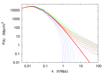
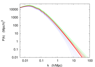
Figure 1: (Left) Matter power spectrum for a family of mixed AD+CDI models, with all parameter fixed except $\alpha$ and $\beta$ (the global normalization also varies in order to mantain a fixed amplitude on large scales). In particular, in all models we kept $n_{\rm ad}=0.95$, $n_{\rm iso}=3$ and $n_{\rm cor}=0$. The thick line stands for the pure adiabatic case ($\alpha=0$). The thin solid (red) lines show uncorrelated models ($\beta=0$) with $\alpha=0.1,0.2,0.3,0.4,0.5,0.6$. The lower blue (upper green) dashed lines show the maximally correlated models with $\beta=1$ (anti-correlated with $\beta=-1$) for the same values of $\alpha$. (Right) Same as the left plot, but with $n_{\rm iso}$ reduced to $2.2$.

III Probing the matter power spectrum with the Lyman-$\alpha$ forest in QSO absorption spectra

It is well established by analytical calculation and hydrodynamical simulations that the Lyman-$\alpha$ forest blueward of the Lyman-$\alpha$ emission line in QSO spectra is produced by the inhomogeneous distribution of a warm ($\sim 10^{4}$ K) and photoionized intergalactic medium (IGM) along the line of sight. The opacity fluctuations in the spectra arise from fluctuations in the matter density and trace the gravitational clustering of the matter distribution in the quasi-linear regime bi . The Lyman-$\alpha$ forest has thus been used extensively as a probe of the matter power spectrum on comoving scales of $(1-40)\,h^{-1}$Mpc bi ; croft ; vhs ; mcdonald2 .

The Lyman-$\alpha$ optical depth in velocity space $u$ (km/s) is related to the neutral hydrogen distribution in real space as (see e.g. Ref. hgz ):

$$\tau(u)={\sigma_{0,\alpha}~{}c\over H(z)}\int_{-\infty}^{\infty}dy\,n_{\rm HI}(y)~{}{\cal V}\left[u-y-v_{\parallel}(y),\,b(y)\right]dy\;,$$ (11)

where $\sigma_{0,\alpha}=4.45\times 10^{-18}$ cm² is the hydrogen Ly$\alpha$ cross-section, $y$ is the real-space coordinate (in km s^-1), ${\cal V}$ is the standard Voigt profile normalized in real-space, $b=(2k_{B}T/mc^{2})^{1/2}$ is the velocity dispersion in units of $c$, $H(z)$ the Hubble parameter, $n_{\rm HI}$ is the local density of neutral hydrogen and $v_{\parallel}$ is the peculiar velocity along the line-of-sight. The density of neutral hydrogen can be obtained by solving the photoionization equilibrium equation (see e.g. katz ). The neutral hydrogen in the IGM responsible for the Lyman-$\alpha$ forest absorptions is highly ionized due to the metagalactic ultraviolet (UV) background radiation produced by stars and QSOs at high redshift. This optically thin gas in photoionization equilibrium produces a Lyman-$\alpha$ optical depth of order unity.

The balance between the photoionization heating by the UV background and adiabatic cooling by the expansion of the universe drives most of the gas with $\delta_{b}<10$, which dominates the Lyman-$\alpha$ opacity, onto a power-law density relation $T=T_{0}\,(1+\delta_{b})^{\gamma-1}$, where the parameters $T_{0}$ and $\gamma$ depend on the reionization history and spectral shape of the UV background and $\delta_{b}$ is the local gas overdensity ($1+\delta_{b}=\rho_{b}/\bar{\rho}_{b}$).

The relevant physical processes can be readily modelled in hydrodynamical simulations. The physics of a photoionized IGM that traces the dark matter distribution is, however, sufficiently simple that considerable insight can be gained from analytical modeling of the IGM opacity based on the so called Fluctuating Gunn Peterson Approximation neglecting the effect of peculiar velocities and the thermal broadening fgpa . The Fluctuating Gunn Peterson Approximation makes use of the power-law temperature density relation and describes the relation between Lyman-$\alpha$ opacity and gas density (see rauch ; croft ) along a given line of sight as follows,

$$\tau(z)\propto(1+\delta_{b}(z))^{2}\,T^{-0.7}(z)={\cal A}(z)\,(1+\delta_{b}(z))^{\beta}\,,$$ (12)

$${\cal A}(z)=0.433\left(\frac{1+z}{3.5}\right)^{6}\left(\frac{\Omega_{b}h^{2}}{0.02}\right)^{2}\left(\frac{T_{0}}{6000\;{\rm K}}\right)^{-0.7}\times$$

$$\hskip 17.07164pt\left(\frac{h}{0.65}\right)^{-1}\left(\frac{H(z)/H_{0}}{3.68}\right)^{-1}\left(\frac{\Gamma_{\rm HI}}{1.5\times 10^{-12}\;{\rm s}^{-1}}\right)^{-1}\,,$$

where $\beta\equiv 2-0.7\,(\gamma-1)$ in the range $1.6-1.8$, $\Gamma_{\rm HI}$ the HI photoionization rate, $H_{0}=h\,100$ km/s/Mpc the Hubble parameter at redshift zero. For a quantitative analysis, however, full hydrodynamical simulations, which properly simulate the non-linear evolution of the IGM and its thermal state, are needed.

Equations (11) and (12) show how the observed flux $F=\exp{(-\tau)}$ depends on the underlying local gas density $\rho_{b}$, which in turn is simply related to the dark matter density, at least at large scales where the baryonic pressure can be neglected gh . Statistical properties of the flux distribution, such as the flux power spectrum, are thus closely related to the statistical properties of the underlying matter density field.

III.1 The data: from the quasar spectra to the flux power spectrum

The power spectrum of the observed flux in high-resolution Lyman-$\alpha$ forest data provides meaningful constraints on the dark matter power spectrum on scales of $0.003\,{\rm s/km}<k<0.03\,{\rm s/km}$, roughly corresponding to scales of $(1-40)\,h^{-1}$Mpc (somewhat dependent on the cosmological model). At larger scales the errors due to uncertainties in fitting a continuum (i.e. in removing the long wavelength dependence of the spectrum emitted by each QSO) become very large while at smaller scales the contribution of metal absorption systems becomes dominant (see e.g. kim04 ; mcdonald ). In this paper, we will use the dark matter power spectrum that Viel, Haehnelt & Springel vhs (VHS) inferred from the flux power spectra of the Croft et al. croft (C02) sample and the LUQAS sample of high-resolution Lyman-$\alpha$ forest data luqas . The C02 sample consists of 30 Keck high resolution HIRES spectra and 23 Keck low resolution LRIS spectra and has a median redshift of $z=2.72$. The LUQAS sample contains 27 spectra taken with the UVES spectrograph and has a median redshift of $z=2.125$. The resolution of the spectra is 6 km/s, 8 km/s and 130 km/s for the UVES, HIRES and LRIS spectra, respectively. The S/N per resolution element is typically 30-50. Damped and sub-damped Lyman-$\alpha$ systems have been removed from the LUQAS sample and their impact on the flux power spectrum has been quantified by croft . Estimates for the errors introduced by continuum fitting, the presence of metal lines in the forest region and strong absorptions systems have also been made mcdonald ; croft ; hui ; kim04 .

III.2 From the flux power spectrum to the linear matter power spectrum

VHS have used numerical simulation to calibrate the relation between flux power spectrum and linear dark matter power spectrum with a method proposed by C02 and improved by gnedham and VHS. A set of hydrodynamical simulations for a coarse grid of the relevant parameters is used to find a model that provides a reasonable but not exact fit to the observed flux power spectrum. Then, it is assumed that the differences between the model and the observed linear power spectrum depend linearly on the matter power spectrum.

The hydrodynamical simulations are used to determine a bias function between flux and matter power spectrum: $P_{F}(k)=b_{F}^{2}(k)\;P(k)$, on the range of scales of interest. In this way the linear matter power spectrum can be recovered with reasonable computational resources. This method has been found to be robust provided the systematic uncertainties are properly taken into account vhs ; gnedham . Running hydrodynamical simulations for a fine grid of all the relevant parameters is unfortunately computationally prohibitive (see discussion in vh on a possible attempt to overcome this problem).

We have seen in section II.3 that the isocurvature mode contribution can create distortions in the small-scale linear matter power spectrum. Of course, this extra freedom was not taken into account in the definition of the grid of models in VHS. In principle, we should run simulations for a new grid with extra parameters ($\alpha$, $\beta$, $n_{\rm iso}$, $n_{\rm cor}$). Alternatively, we can carry a tentative analysis with the same function $b_{F}(k)$ and the same error bars as in the pure adiabatic case, and check the validity of our results a posteriori. The idea is simply to select a marginally excluded model with the largest possible deviation from adiabaticity in the matter power spectrum. For this model, we run a new hydrodynamical simulation and we compare $P_{F}(k)/P(k)$ with the function $b_{F}^{2}(k)$ used in the analysis. In case of good agreement, the results will be validated. We expect this agreement to be fairly good on large scales, but deviations should appear on small scales, because of the different non-linear evolution.

The use of state-of-the-art hydrodynamical simulations is a significant improvement compared to previous studies which used numerical simulation of dark matter only croft . We use the parallel TreeSPH code GADGET-II volker in its TreePM mode which speeds up the calculation of long-range gravitational forces considerably. The simulations are performed with periodic boundary conditions with an equal number of dark matter and gas particles. Radiative cooling and heating processes are followed using an implementation similar to katz for a primordial mix of hydrogen and helium. The UV background is given by haardt . To maximise the speed of the simulation a simplified criterion of star formation has been applied: all the gas at overdensities larger than 1000 times the mean overdensity is turned into stars vhs . The simulations were run on cosmos, a 152 Gb shared memory Altix 3700 with 152 CPUs hosted at the Department of Applied Mathematics and Theoretical Physics (Cambridge).

III.3 Systematics Errors

There is a number of systematic uncertainties and statistical errors which affect the inferred power spectrum and an extensive discussion can be found in croft ; gnedham ; vhs ; vh . VHS estimated the uncertainty of the overall rms fluctuation amplitude of matter fluctuation to be 14.5 % with a wide range of different factors contributing.

We present here a brief summary. The effective optical depth, $\tau_{\rm eff}=-\ln\langle F\rangle$ which is essential for the calibration procedure has to be determined separately from the absorption spectra. As discussed in VHS, there is a considerable spread in the measurement of the effective optical depth in the literature. Determinations from low-resolution low S/N spectra give systematically higher values than high-resolution high S/N spectra. However, there is little doubt that the lower values from high-resolution high S/N spectra are appropriate and the range suggested in VHS leads to a 8% uncertainty in the rms fluctuation amplitude of the matter density field (see Table 5 in VHS). Other uncertainties are the slope and normalization of the temperature-density relation of the absorbing gas which is usually parametrised as $T=T_{0}\,(1+\delta_{b})^{\gamma-1}$. $T_{0}$ and $\gamma$ together contribute up to 5% to the error of the inferred fluctuation amplitude. VHS further estimated that uncertainties due to the C02 method (due to fitting the observed flux power spectrum with a bias function which is extracted at a slightly different redshift than the observations) contribute about 5%. They further assigned a 5 % uncertainty to the somewhat uncertain effect of galactic winds and finally an 8% uncertainty due the numerical simulations (codes used by different groups give somewhat different results). Summed in quadrature, all these errors led to the estimate of the overall uncertainty of 14.5% in the rms fluctuation amplitude of the matter density field.

For our analysis we use the inferred DM power spectrum in the range $0.003\,{\rm s/km}<k<0.03\,{\rm s/km}$ as given in Table 4 of VHS. (Note that, as in  vielandjulien05 we have reduced the power spectrum values by 7% to mimick a temperature-density relation with $\gamma=1.3$, the middle of the plausible range for $\gamma$ temperature ).

Unfortunately at smaller scales the systematic errors become prohibitively large mainly due to the large contribution of metal absorption lines to the flux power spectrum (see Fig. 3 of Ref. vhs ) and due to the much larger sensitivity of the flux power spectrum to the thermal state of the gas at these scales.

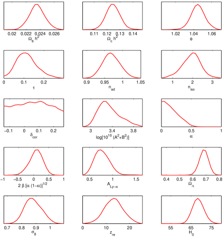
Figure 2: Likelihood for the AD+CDI model, using all our data set. The first eleven parameters are independent, while the last four are related parameters (with non-flat priors).

parameter	$1\sigma$ C.L.
$\Omega_{b}h^{2}$	0.0235 $\pm$ 0.0011
$\Omega_{c}h^{2}$	0.125 $\pm$ 0.005
$\theta$	1.045 $\pm$ 0.008
$\tau$	0.11 $\pm$ 0.05
$n_{\rm ad}$	0.97 $\pm$ 0.02
$n_{\rm iso}$	1.9 $\pm$ 0.5
$\delta_{\rm cor}$	within prior range
$\log[10^{10}(A^{2}+B^{2})]$	3.3 $\pm$ 0.2
$\alpha$	$<0.20$
$2\beta[\alpha(1-\alpha)]^{1/2}$	0.1 $\pm$ 0.2
$A_{{\rm Ly}-\alpha}$	0.8 $\pm$ 0.2
$\Omega_{\Lambda}$	0.68 $\pm$ 0.03
$\sigma_{8}$	0.88 $\pm$ 0.06
$z_{\rm re}$	13 $\pm$ 4
$H_{0}$	69 $\pm$ 3

Table 1: $1\sigma$ confidence limits for the AD+CDI model, using all our data set, for the eleven basis parameters with flat priors, and below, for related parameters.

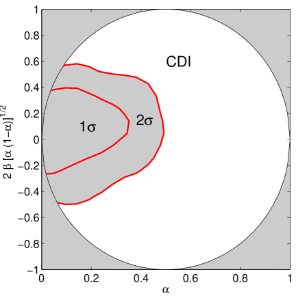
Figure 3: Two-dimensional likelihood for the amplitude of the isocurvature mode and of the cross-correlation component, near the pivot scale. We adopted a flat prior within the ellipse (which appears here as a circle) in which these parameters are defined.

IV Fitting the data

IV.1 Parameter basis and priors

Any AD+CDI model is described by the usual six parameters of the $\Lambda$CDM model, plus four parameters for the isocurvature sector (two amplitudes and two tilts). Like in most of the literature, we define the amplitudes parameters at the pivot scale $k_{0}=0.05\,$Mpc^-1. For the isocurvature fraction, we could decide to impose a flat prior on $f_{\rm iso}$, or $\alpha$, or any function of them; different choices are not equivalent, in general. We will come back to the dependence of the final result on the choice of priors in section IV.5. Meanwhile, we chose a specific set of parameters which appear linearly in the expression of the observable power spectra, $\alpha$ and $2\beta\sqrt{\alpha(1-\alpha)}$, and that we believe are physically relevant. As already mentioned, these two parameter are defined within an ellipse, in which we assume a flat prior. Furthermore, we must take into account the inequality

$$\left|\cos\Delta\right|=\left|\beta\right|\left({k\over k_{0}}\right)^{n_{\rm cor}}\leq 1$$ (13)

which should hold at least over the scales probed by the data, i.e. typically between $k_{\rm min}=4\times 10^{-5}$Mpc^-1 and $k_{\rm max}=2\,$Mpc^-1. This is achieved by introducing a new parameter $\delta_{\rm cor}\equiv n_{\rm cor}/\ln|\beta|^{-1}$, with a flat prior within the range $-0.14<\delta_{\rm cor}<0.27$. In summary, our basis parameters with flat priors consists of:

• the baryon density, $\omega_{\rm b}=\Omega_{\rm b}h^{2}$,

• the cold dark matter density, $\omega_{c}=\Omega_{c}h^{2}$,

• the ratio $\theta$ of the sound horizon to the angular diameter distance multiplied by 100,

• the optical depth to reionization, $\tau$,

• the adiabatic tilt, $n_{\rm ad}$,

• the isocurvature tilt, $n_{\rm iso}$,

• the parameter related to the tilt of the cross-correlation angle, $\delta_{\rm cor}\in[-0.14,0.27]$,

• the overall normalization, $\ln[10^{10}(A^{2}+B^{2})]$,

• the isocurvature fraction, $\alpha$,

• the cross-correlation amplitude, $2\beta\sqrt{\alpha(1-\alpha)}$.

In addition, there are three independent parameters related to observations: the Lyman-$\alpha$ calibration parameter $A_{{\rm Ly}-\alpha}$ defined in vwh , on which we impose the same Gaussian prior $A_{{\rm Ly}-\alpha}=1.0\pm 0.29$; and the two bias parameters associated to the 2dF and SDSS data with flat priors. Our full parameter space is therefore 13-dimensional.

IV.2 Results

We compute the marginalized Bayesian likelihood of each parameter with a Monte Carlo Markov Chain method, using the public code CosmoMC cosmomc . The results are displayed in Fig. 2 and Table 1 (after marginalization over the 2dF and SDSS bias parameters). The data favors purely adiabatic models, but remains compatible with an isocurvature fraction $\alpha<0.40$ at the 2$\sigma$ (95%) confidence level (CL), with a tilt $n_{\rm iso}=1.9\pm 1.0$ ($2\sigma$ CL). The one-dimensional likelihoods for $\alpha$, $2\beta\sqrt{\alpha(1-\alpha)}$ must be interpreted with care: the fact that these parameters are defined within an ellipse implies that there is more parameter space available near $\alpha=0.5$ and $2\beta\sqrt{\alpha(1-\alpha)}=0$. More interesting are the two-dimensional likelihood contours for $(\alpha,\,2\beta\sqrt{\alpha(1-\alpha)})$ displayed in Fig. 3, since in this representation the prior is really flat inside the ellipse. From this figure, it is clear that the data prefers an uncorrelated isocurvature contribution. The flatness of the $\delta_{\rm cor}$ likelihood shows that the data give no indication on the tilt of the cross-correlation angle.

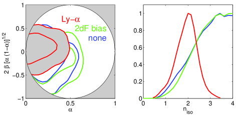
Figure 4: Likelihood of the isocurvature-related parameters, for the three combinations of data sets described in section IV.3: “Lyman-$\alpha$” (red), “2dF bias prior” (green) and “none” (blue). (Left) Marginalized 1$\sigma$ and 2$\sigma$ confidence levels in the $(\alpha,2\beta[\alpha(1-\alpha)]^{1/2})$ space. (Right) Marginalized probability distribution for $n_{\rm iso}$.

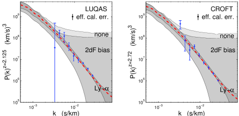
Figure 5: Favored ranges for the matter power spectrum $P(k)$ in the three runs “Lyman-$\alpha$” (dark), “2dF bias prior” (medium) and “none” (light), compared with our Lyman-$\alpha$ data, from the LUQAS quasar spectra (left) and from the re-analyzed Croft et al. spectra (right). The bands represent the envelope of all the matter power spectra in the Markov chains (after eliminating models with the worse likelihood). Each power spectrum has been computed at the median redshift of the data and re-expressed in units of km/s. In addition to the statistical errors, the data points share an overall effective calibration error, whose standard deviation is displayed in the top right corners. For the run including the Lyman-$\alpha$ data, each power spectrum has been divided by the value of the calibration parameter. The red dashed curves show the particular power spectrum discussed in section IV.4.

IV.3 Specific impact of the Ly-$\alpha$ data

The Lyman-$\alpha$ forest provides a powerful indication on both the amplitude and the shape of the matter power spectrum for $k>0.01$ s/km, i.e. roughly larger than $1h/$Mpc. In order to illustrate the importance of this data set in our results, we repeat the same analysis without Lyman-$\alpha$ data. In this case, there are two options: we can either use the 2dF and SDSS galaxy power spectrum data as a constraint only on the shape of the matter power spectrum, as already done in the previous analysis of section IV.2; or introduce a bias prior derived e.g. from the third and fourth-order galaxy correlation function of the 2dF catalogue 2dFGRS ; Verde2003 , in order to keep an information on the amplitude of the matter power spectrum.

For these three cases, that we call “Lyman-$\alpha$”, “2dFbias prior” and “none”, the 2$\sigma$ upper bound on $\alpha$ are respectively equal to 0.4, 0.5 and 0.5. The likelihoods for the most interesting parameters are displayed in Fig. 4. As expected, the Lyman-$\alpha$ data set is significanty more powerful than the 2dF bias prior for cutting out models with large $\alpha$, and even more clearly, with large $n_{\rm iso}$ or large anticorrelation, as can be seen in Fig. 4. It is important to note that without these data, all results depend on our arbitrary prior $n_{\rm iso}<4$: values far beyond this upper bound could still be compatible with the data, as also found in Ref. Kurki-Suonio:2004mn when using the same pivot scale. In the presence of the Lyman-$\alpha$ data, we get a robust upper bound on $n_{\rm iso}$, and none of our priors play a role in the final results, with the exception of the well-motivated $\delta_{\rm cor}$ prior.

The impact of the Lyman-$\alpha$ data can be understood visually from Fig. 5. After running each case, we consider the collection of all matter power spectra in our Markhov chains (except models with a bad posterior likelihood ${\cal L}<{\cal L}_{\rm max}/5$). The gray bands in Fig. 5 correspond to the envelope of all these $P(k)$’s, compared to the Lyman-$\alpha$ data points. As expected, when the Lyman-$\alpha$ is not used, the band gets very wide above the wavenumber $k\sim 0.2~{}h/$Mpc$~{}\sim 2\times 10^{-3}\,$s/km (note that for models with $n_{\rm iso}=4$, the small-scale power spectrum is asymptotically flat). The role of the bias prior is marginal: it simply favors models with the lowest global normalization, but without affecting the isocurvature fraction and tilt. Using the Lyman-$\alpha$ data, we can exclude any break in the power spectrum on scales $k\leq 3~{}h/$Mpc$~{}\sim~{}3\times 10^{-2}\,$s/km. This results in much stronger constraints for the parameters $(\alpha,\beta,n_{\rm iso})$, as can be seen from Fig. 4.

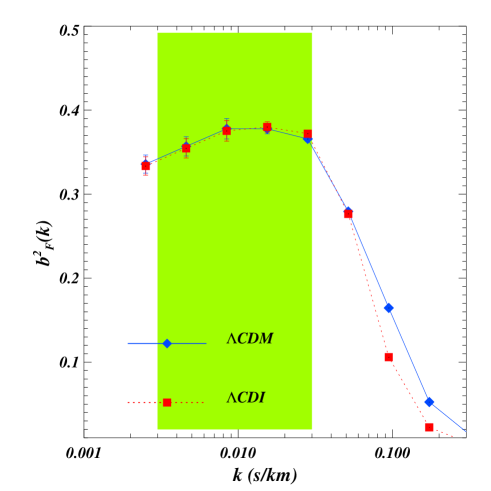
Figure 6: The ratio $b_{F}(k)^{2}\equiv P_{\rm flux}(k)/P_{\rm matter}(k)$ at $z=2.75$, computed from the hydrodynamical simulations as the ratio of the flux power spectrum (averaged over 1000 line-of-sights) over the input linear matter power spectrum. The solid blue curve shows the result for an adiabatic $\Lambda$CDM close to the best-fit model, while the dashed red curve was obtained from the “most extreme AD+CDI mixed model” defined in section IV.4 and here labelled as $\Lambda$CDI. The green band shows the region in which the Lyman-$\alpha$ data is used in the present analysis.

IV.4 Checking the validity of the Ly-$\alpha$ data fitting procedure

We apply the strategy described in section III.2 in order to check the validity of our Lyman-$\alpha$ data fitting procedure. We take the large number of samples contained in our Markov chains, and eliminate all models with a likelihood smaller than ${\cal L}_{\rm max}/10$ (in terms of effective $\chi^{2}$, this corresponds to $\Delta\chi^{2}=\chi^{2}-\chi_{\rm min}^{2}>20$). We then select the model with the largest value of $\alpha$, which represents the strongest deviation from the purely adiabatic model. The corresponding matter power spectrum is plotted in Fig. 5 and has a break around $k\sim 5~{}h/$Mpc$~{}\sim 5\times 10^{-2}\,$s/km. Above this wavenumber, the slope of the power spectrum is given by eq. (10) with $n_{\rm iso}=2.7$. For this “extreme” model, we perform a hydrodynamical simulation as described in section III.2, and compare the bias function $b_{F}(k)$ with that assumed throughout the analysis. As shown in Fig.6, in the range $0.003<k<0.3\,$km/s probed by the data, the difference between the two functions is very small with respect to the statistical errors on the data. We conclude that in the present context, our Lyman-$\alpha$ data fitting procedure is robust, and does not introduce an error in the 1$\sigma$ or 2$\sigma$ bounds derived for each parameter of the AD+CDI mixed model.

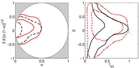
Figure 7: Two-dimensional 68% and 95% confidence limits for the CDI mode amplitude and cross-correlation angle (evaluated at the pivot scale). The two plots show the results of two independent runs with different parameter basis and priors. On the left (solid red curves), the parameters are $(\alpha,\,2\beta\sqrt{\alpha(1-\alpha)})$, with a flat prior within the ellipse. On the right (solid black lines), the parameters are $(f_{\rm iso},\cos\Delta)$, related to the previous parameters through eqs.(6), with a flat prior within the square. The dashed curves show for comparison the likelihood contours obtained for one parameter set, assuming a flat prior on the other parameter set.

IV.5 The role of parametrization and priors

The fact of choosing a top-hat prior in the $(\alpha,\,2\beta\sqrt{\alpha(1-\alpha)})$ parameter space is rather arbitrary. Other groups prefer to take top-hat priors on $f_{\rm iso}$, defined in Eq.(6), and $\cos\Delta=\beta$. Due to the non-linear transformation between the two basis, they are clearly not equivalent in terms of priors (see the discussion of this point in Trotta:2005ar , in the context of Bayesian Evidence calculation for adiabatic versus mixed models).

We checked this issue explicitly with an independent run based on the $(f_{\rm iso},\cos\Delta)$ basis. The results are summarized in Fig. 7. As expected from the Jacobian, the $(f_{\rm iso},\cos\Delta)$ option gives more weight to models with a small isocurvature fraction. For instance, the run with a flat prior on $f_{\rm iso}$ gives a 1$\sigma$ bound $f_{\rm iso}<0.26$, while that with a flat prior on $\alpha$ gives $f_{\rm iso}<0.66$. However, at the 2$\sigma$ level, the relative difference is small ($f_{\rm iso}<0.75$ versus $f_{\rm iso}<0.87$) because the Jacobian is asymptotically flat.

In principle, in Bayesian analysis, the choice of parameter basis and priors should reflect one’s knowledge on the model before comparision with the data. However, in the absence of a unique underlying physical model motivating the presence of isocurvature modes, different scientists might put foward different choices of prior. This intrinsic freedom in Bayesian analyses should always be kept in mind when quoting bounds, especially for parameters which represent physical ingredients not strictly needed by the data, which is the case here for the isocurvature sector parameters (for other parameters such that the data picks up a narrow allowed region, a change of priors won’t affect the bounds very much). However, even for the isocurvature parameters discussed here, it is reassuring to see from our analysis that the 2$\sigma$ contours obtained from the the two runs and compared in Fig. 7 are roughly in agreement.

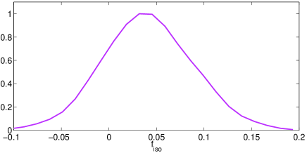
Figure 8: Likelihood for $f_{\rm iso}$ in the curvaton model.

IV.6 The curvaton model

In this section we derive bounds on the specific case of curvaton models. The curvaton hypothesis is an ingenuous way to generate the observed curvature perturbation from a field (the curvaton) different from that which drives inflation (the inflaton) Lyth:2001nq . In practice there is not much difference in the phenomenological signatures left in the CMB and LSS compared to an ordinary inflationary model. However, there are a few cases in which it is possible to leave a “residual” isocurvature component, together with the dominant curvature contribution. More specifically, in the curvaton models in which the curvaton field is responsible for the CDM component of matter, there are various possibilities depending on the time of creation of CDM versus the decay of the curvaton field. In all these cases, the curvature and isocurvature perturbations are related to the gauge invariant Bardeen variable $\zeta$ as

$${\cal S}=3(\zeta_{\rm cdm}-\zeta)\,,$$ (14)

$${\cal R}=-\zeta\,.$$ (15)

Let us classify here the different cases: 1) when CDM-creation occurs before the curvaton decays and the fraction $r$ of the total energy density in the curvaton field at the time of its decay is negligible. Then ${\cal S}=-3\zeta=3{\cal R}$, which corresponds to $f_{\rm iso}=3$ ($\alpha=0.9$), and $\beta=+1$ (maximally correlated), with $n_{\rm iso}=n_{\rm ad}$; 2) when CDM-creation occurs before the curvaton decays but the fraction $r$ at decay is important. This case requires specific model input and in principle can have any value of $f_{\rm iso}$ and $\beta$, while $n_{\rm iso}=n_{\rm ad}$; 3) when CDM-creation occurs at the decay of the curvaton and the fraction $r<1$. In this case, $\zeta_{\rm cdm}=\zeta/r$ and thus ${\cal S}=3(r^{-1}-1)\zeta=3(1-1/r){\cal R}$, which corresponds to $f_{\rm iso}=3(1-1/r)$, i.e. $\beta=-1$ (maximally anticorrelated) and $n_{\rm iso}=n_{\rm ad}$; 4) when CDM-creation occurs after the curvaton decay. Then there is only one thermal fluid in equilibrium, $\zeta_{\rm cdm}=\zeta$, and there is no way to generate an isocurvature perturbation, ${\cal S}=0$.

Since case 1) is already excluded at many sigma, and case 2) is essentially identical (except for $n_{\rm iso}=n_{\rm ad}$) to our generic analysis, we will concentrate on case 3) of a maximally anticorrelated mixture of isocurvature and adiabatic modes with equal tilts and $\delta_{\rm cor}=0$. Our results are summarized in Fig. 8, which shows the likelihood distribution for the generic curvaton model. We have used $n_{\rm ad}=n_{\rm iso}$, $\delta_{\rm cor}=0$, and $\beta=\pm 1$, which is equivalent to $\beta=1$ and $f_{\rm iso}$ positive or negative: $f_{\rm iso}>0$ corresponds to $\beta=1$, or positive correlation between ${\cal R}_{\rm rad}$ and ${\cal S}_{\rm rad}$, i.e. suppression of power in $P(k)$ and in the large-scale CMB temperature spectrum; while $f_{\rm iso}<0$ corresponds to the opposite anti-correlated case.

We find $f_{\rm iso}=0.04\pm 0.09$ at the 2$\sigma$-level, which implies $r>0.98$ at the same CL. In our opinion, such a stringent constraint on the fraction of energy density in the curvaton at decay calls for a tremendous finetuning (there is no physical reason to expect that the curvaton should decay precisely when it is starting to dominate the total energy density of the universe, within 2%), which makes the curvaton hypothesis in its most attractive scenario very unlikely.

IV.7 The double inflation model

Another chance to generate an observable isocurvature signature is through the possible presence of two scalar fields driving inflation Polarski:1994rz ; double . The simplest case at hand is that of two massive fields coupled only gravitationally:

$$\mathcal{L}=\frac{1}{2}(\phi_{h;\mu}\phi_{h}^{;\mu}-m_{h}^{2}\phi^{2}_{h})+\frac{1}{2}(\phi_{l;\mu}\phi_{l}^{;\mu}-m_{l}^{2}\phi^{2}_{l})~{},$$ (16)

where $m_{h}$ and $m_{l}$ are the masses of the heavy and light fields respectively.

We assume slow-roll conditions during inflation, and use the number of e-folds till the end of inflation $s=-\ln(a/a_{\rm end})$ to parametrize the fields as:

$$\phi_{h}^{2}=\frac{s}{2\pi G}\sin^{2}\theta;~{}\phi_{l}^{2}=\frac{s}{2\pi G}\cos^{2}\theta~{},$$ (17)

Using the field and Friedmann equations, we can solve for the rate of expansion during inflation:

$$H^{2}(s)\simeq\frac{2}{3}s\cdot m_{l}^{2}[1+(R^{2}-1)\sin^{2}\theta]~{},$$ (18)

where $R=m_{h}/m_{l}$, and find the number of e-folds as a function of $\theta$:

$$s(\theta)=s_{0}\frac{(\sin\theta)^{2/(R^{2}-1)}}{(\cos\theta)^{2R^{2}/(R^{2}-1)}}~{}.$$ (19)

The perturbed Einstein equations can be solved for long wavelength modes in the longitudinal gauge. Assuming that the heavy field decays into CDM whereas the ligth field produces other species, we find the magnitudes of the curvature and entropy perturbation at horizon crossing. During radiation domination and for super-Hubble modes, this gives:

$${\cal R}_{\rm rad}(k) = -\sqrt{\frac{4\pi G}{k^{3}}}H_{k}s_{k}^{1/2}\Big{(}\sin\theta_{k}\,e_{h}({\bf k})+\cos\theta_{k}\,e_{l}({\bf k})\Big{)}\,$$

$${\cal S}_{\rm rad}(k) = \sqrt{\frac{4\pi G}{k^{3}}}H_{k}s_{k}^{-1/2}\left({e_{h}({\bf k})\over\sin\theta_{k}}-{R^{2}\,e_{l}({\bf k})\over\cos\theta_{k}}\right)\,$$ (20)

where $e_{i}({\bf{k}})$ are gaussian random fields associated with the quantum fluctuations of the fields, and the subindex $k$ implies the value of the corresponding quantity at horizon crossing during inflation. One typically expects $s_{k}\simeq 60$. It can be seen from (II.1) that the correlation power spectrum has no scale dependence, and thus, for this model $n_{\rm cor}=0$, while the adiabatic and isocurvature tilts have expressions

$$n_{\rm ad} = 1-{2\over s_{k}}+{(R^{2}-1)\tan^{2}\theta\over 2s_{k}(1+R^{2}\tan^{2}\theta)^{2}}\,,$$ (21)

$$n_{\rm iso} = 1-{(R^{2}-1)(R^{2}\tan^{4}\theta-1)(1+\tan^{2}\theta)\over s_{k}(1+R^{2}\tan^{2}\theta)^{2}(1+R^{4}\tan^{2}\theta)}\,,$$ (22)

whose values, for $s_{k}=60$, are typically $n_{\rm ad}=0.97$ and $n_{\rm iso}$ in the range $[0.97,0.90]$ for $R\in[1,4]$. Since $n_{\rm iso}>0.93$ at 95% c.l., models with large values of $R$ are ruled out.

It was shown in Beltran:2004uv that a relationship beteween $\alpha$ and $\beta$ can be found. It can be simply expressed as a straight line in our parameter space:

$$2\beta\sqrt{\alpha(1-\alpha)}=\frac{2(R^{2}-1)}{s_{k}}(1-\alpha)\,.$$ (23)

On the other hand, for these models, the parameters $\alpha$ and $\beta$ have minimum and maximum values respectively, which only depend on the ratio $R$ and the number of e-folds $s_{k}$,

$$\alpha_{\rm min} = {(R^{2}+1)^{2}\over s_{k}^{2}+(R^{2}+1)^{2}}\,,$$ (24)

$$\beta_{\rm max} = {R^{2}-1\over R^{2}+1}\,,$$ (25)

$$\left.2\beta\sqrt{\alpha(1-\alpha)}\right|_{\rm max} = {2s_{k}(R^{2}-1)\over s_{k}^{2}+(R^{2}+1)^{2}}\,.$$ (26)

Using the results of section IV.2, we find that the inclusion of the Lyman-$\alpha$ data significantly improves the previous bound on R to $R<3$ at 95% c.l. This bound comes mainly from a combination of bounds on $2\beta\sqrt{\alpha(1-\alpha)}$ and $n_{\rm iso}$.

We did not find necessary to generate a $n_{\rm cor}=0$ sampling for this model. In our results, the parameter $\delta_{\rm cor}$ has a flat distribution and thus is unconstrained. We therefore expect similar results when fixing it to zero.

V Conclusions

In addition to CMB, LSS and SNIa data, we used some recent Lyman-$\alpha$ forest data to further constrain the bounds on possible CDM-isocurvature primordial fluctuations. We find that the systematics induced $-$ in particular, those associated with the recovery of the linear dark matter power spectrum from the flux power spectrum $-$ are greatly compensated by the valuable information on the small-scale matter power spectrum provided by the Lyman-$\alpha$ data.

Before summarizing our results, it is worth mentioning that when we omit the Lyman-$\alpha$ forest data our bounds agree very well with those of Ref. Kurki-Suonio:2004mn . The authors of Kurki-Suonio:2004mn work with a pivot scale $k_{0}=0.02~{}$Mpc^-1, but they also show how their results are modified when they take $k_{0}=0.05~{}$Mpc^-1 like in the present paper: in that case the agreement with us is particularly good. The comparison of our results with the WMAP analysis from Ref. Peiris is more puzzling: using or not some Lyman-$\alpha$ data, they always find much stronger bounds on $f_{\rm iso}$ than us. It is true that we have one more free parameter $\delta_{\rm cor}$, and that we do not introduce a prior on the 2dF bias; however, even when we fix $\delta_{\rm cor}=0$ and introduce such a prior, our $f_{\rm iso}$ bound remains much weaker. So far, private communications with the WMAP team did not allow us to understand the origin of the discrepancy.

Using all our data set, we find at the 95% confidence level, an isocurvature fraction $\alpha<0.4$, a cross-correlation amplitude $2\beta\sqrt{\alpha(1-\alpha)}=0.1\pm 0.4$, and an isocurvature tilt $n_{\rm iso}=1.9\pm 1.0$. The tilt of the correlation angle remains unconstrained. If we switch to the basis used for instance in Ref. Peiris we find $f_{\rm iso}<0.75$ at 95% c.l.

In the case of a curvaton scenario where CDM-creation occurs at the decay of the curvaton – a case in which the adiabatic and isocurvature modes are maximally anti-correlated, $\beta=-1$, and $n_{\rm ad}=n_{\rm iso}$ – we find $f_{\rm iso}<0.05$, still at the 95% confidence level. This requires that the fraction $r$ of the total density in the curvaton field at that time be fine-tuned between 0.98 and one. Finally, if we assume a double-inflation model with two massive inflatons coupled only gravitationally, such that the heaviest field decays into CDM, while the lightest one into standard model particles, we find that the mass ratio should obey $R<3$ (95% c.l.).

References

- (1) A. D. Linde, Phys. Lett. B 158, 375 (1985); L. A. Kofman and A. D. Linde, Nucl. Phys. B 282, 555 (1987); S. Mollerach, Phys. Lett. B 242, 158 (1990); A. D. Linde and V. Mukhanov, Phys. Rev. D 56, 535 (1997); M. Kawasaki, N. Sugiyama and T. Yanagida, Phys. Rev. D 54, 2442 (1996); P. J. E. Peebles, Astrophys. J. 510, 523 (1999).
- (2) D. Polarski and A. A. Starobinsky, Phys. Rev. D 50, 6123 (1994); M. Sasaki and E. D. Stewart, Prog. Theor. Phys. 95, 71 (1996); M. Sasaki and T. Tanaka, Prog. Theor. Phys. 99, 763 (1998).
- (3) J. García-Bellido and D. Wands, Phys. Rev. D 53, 5437 (1996); 52, 6739 (1995).
- (4) C. Gordon, D. Wands, B. A. Bassett and R. Maartens, Phys. Rev. D 63, 023506 (2001); N. Bartolo, S. Matarrese and A. Riotto, Phys. Rev. D 64, 123504 (2001).
- (5) D. Wands, N. Bartolo, S. Matarrese and A. Riotto, Phys. Rev. D 66, 043520 (2002).
- (6) F. Finelli and R. H. Brandenberger, Phys. Rev. D 62, 083502 (2000); F. Di Marco, F. Finelli and R. Brandenberger, Phys. Rev. D 67, 063512 (2003).
- (7) D. Langlois, Phys. Rev. D 59, 123512 (1999); D. Langlois and A. Riazuelo, Phys. Rev. D 62, 043504 (2000).
- (8) G. Efstathiou and J. R. Bond, Mon. Not. R. Astron. Soc. A 218, 103 (1986); 227, 33 (1987); P. J. E. Peebles, Nature 327, 210 (1987). H. Kodama and M. Sasaki, Int. J. Mod. Phys. A 1, 265 (1986); 2, 491 (1987); S. Mollerach, Phys. Rev. D 42, 313 (1990).
- (9) M. Bucher, K. Moodley and N. Turok, Phys. Rev. D 62, 083508 (2000); Phys. Rev. Lett. 87, 191301 (2001).
- (10) N. Sugiyama, S. Zaroubi, J. Silk Mon. Not. Roy. Astron. Soc. 354, 543 (2004).
- (11) S. Weinberg, Phys. Rev. D 70, 083522 (2004).
- (12) D. H. Lyth, C. Ungarelli and D. Wands, Phys. Rev. D 67, 023503 (2003).
- (13) C. Gordon and K. A. Malik, Phys. Rev. D 69, 063508 (2004).
- (14) K. Enqvist and M. S. Sloth, Nucl. Phys. B 626, 395 (2002).
- (15) D. H. Lyth and D. Wands, Phys. Lett. B 524, 5 (2002);
- (16) T. Moroi and T. Takahashi, Phys. Lett. B 522, 215 (2001) [Erratum-ibid. B 539, 303 (2002)]; Phys. Rev. D 66, 063501 (2002).
- (17) N. Bartolo, E. Komatsu, S. Matarrese and A. Riotto, Phys. Rept. 402, 103 (2004).
- (18) R. Trotta, A. Riazuelo and R. Durrer, Phys. Rev. Lett. 87, 231301 (2001); Phys. Rev. D 67, 063520 (2003).
- (19) M. Bucher, J. Dunkley, P. G. Ferreira, K. Moodley and C. Skordis, Phys. Rev. Lett. 93, 081301 (2004); K. Moodley, M. Bucher, J. Dunkley, P. G. Ferreira and C. Skordis, Phys. Rev. D 70, 103520 (2004); J. Dunkley, M. Bucher, P. G. Ferreira, K. Moodley and C. Skordis, arXiv:astro-ph/0507473.
- (20) J. Valiviita and V. Muhonen, Phys. Rev. Lett. 91, 131302 (2003).
- (21) M. Beltran, J. Garcia-Bellido, J. Lesgourgues and A. Riazuelo, Phys. Rev. D 70, 103530 (2004).
- (22) H. Kurki-Suonio, V. Muhonen and J. Valiviita, Phys. Rev. D 71, 063005 (2005).
- (23) L. Amendola, C. Gordon, D. Wands and M. Sasaki, Phys. Rev. Lett. 88, 211302 (2002).
- (24) H. V. Peiris et al., Astrophys. J. Suppl. 148, 213 (2003).
- (25) P. Crotty, J. García-Bellido, J. Lesgourgues and A. Riazuelo, Phys. Rev. Lett. 91, 171301 (2003).
- (26) F. Ferrer, S. Rasanen and J. Valiviita, JCAP 0410, 010 (2004).
- (27) D. Parkinson, S. Tsujikawa, B. A. Bassett and L. Amendola, arXiv:astro-ph/0409071.
- (28) C. Gordon and A. Lewis, Phys. Rev. D 67, 123513 (2003); New Astron. Rev. 47, 793 (2003).
- (29) G. Lazarides, R. R. de Austri and R. Trotta, Phys. Rev. D 70, 123527 (2004).
- (30) M. Beltran, J. Garcia-Bellido, J. Lesgourgues, A. R. Liddle and A. Slosar, Phys. Rev. D 71, 063532 (2005).
- (31) R. Trotta, arXiv:astro-ph/0504022.
- (32) T. S. Kim, M. Viel, M. G. Haehnelt, R. F. Carswell and S. Cristiani, Mon. Not. Roy. Astron. Soc. 347, 355 (2004).
- (33) R. A. C. Croft et al., Astrophys. J. 581, 20 (2002).
- (34) M. Viel, M. G. Haehnelt and V. Springel, Mon. Not. Roy. Astron. Soc. 354, 684 (2004).
- (35) C. L. Bennett et al. [WMAP Collaboration], Astrophys. J. Suppl. 148, 1 (2003); D. N. Spergel et al., Astrophys. J. Suppl. 148, 175 (2003);
- (36) R. Rebolo et al. [VSA Collaboration], Mon. Not. Roy. Astron. Soc. 353, 747 (2004); C. Dickinson et al., Mon. Not. Roy. Astron. Soc. 353, 732 (2004).
- (37) T. J. Pearson et al. [CBI Collaboration], Astrophys. J. 591, 556 (2003); J. L. Sievers et al., Astrophys. J. 591, 599 (2003); A. C. S. Readhead et al., Astrophys. J. 609, 498 (2004).
- (38) C. l. Kuo et al. [ACBAR Collaboration], Astrophys. J. 600, 32 (2004); J. H. Goldstein et al., Astrophys. J. 599, 773 (2003).
- (39) J. A. Peacock et al. [2dFGRS Collaboration], Nature 410, 169 (2001); W. J. Percival et al., Mon. Not. R. Astron. Soc. A 327, 1297 (2001); 337, 1068 (2002).
- (40) M. Tegmark et al. [SDSS Collaboration], Astrophys. J. 606, 702 (2004).
- (41) A. G. Riess et al. [Supernova Search Team Collaboration], Astrophys. J. 607, 665 (2004).
- (42) U. Seljak et al., Phys. Rev. D 71, 103515 (2005).
- (43) M. Viel, M.G. Haehnelt arXiv:astro-ph/0508177
- (44) M. Viel, J. Lesgourgues, M.G. Haehnelt, S. Matarrese, A. Riotto, Phys. Rev. D 71, 063534 (2005).
- (45) R. Stompor, A. J. Banday and K. M. Gorski, Astrophys. J. 463, 8 (1996); P. J. E. Peebles, Astrophys. J. 510, 531 (1999); E. Pierpaoli, J. García-Bellido and S. Borgani, JHEP 9910, 015 (1999); M. Kawasaki and F. Takahashi, Phys. Lett. B 516, 388 (2001); K. Enqvist, H. Kurki-Suonio and J. Väliviita, Phys. Rev. D 62, 103003 (2000); 65, 043002 (2002).
- (46) A. R. Liddle and D. H. Lyth, “Cosmological inflation and large-scale structure”, Cambridge University Press (2000); E. Bertschinger, arXiv:astro-ph/0101009;
- (47) H. Bi, Astrophys. J. 405, 479 (1993); M. Viel, S. Matarrese, H. J. Mo, M. G. Haehnelt and T. Theuns, Mon. Not. Roy. Astron. Soc. 329, 848 (2002); M. Zaldarriaga, R. Scoccimarro and L. Hui, Astrophys. J. 590, 1 (2003).
- (48) P. McDonald et al., arXiv:astro-ph/0407377.
- (49) L. Hui, N. Y. Gnedin and Y. Zhang, Astrophys. J. 486, 599 (1997).
- (50) N. Katz, D. H. Weinberg and L. Hernquist, Astrophys. J. Suppl. 105, 19 (1996).
- (51) J. E. Gunn and B. A. Peterson, Astrophys. J. 142, 1633 (1965); J. N. Bahcall and E. E. Salpeter, Astrophys. J. 142, 1677 (1965).
- (52) M. Rauch, ARA&A 36, 267 (1998).
- (53) L. Hui and N. Gnedin, Mon. Not. Roy. Astron. Soc. 292, 27 (1997); N. Y. Gnedin and L. Hui, Mon. Not. Roy. Astron. Soc. 296, 44 (1998).
- (54) P. McDonald et al., arXiv:astro-ph/0405013.
- (55) http://www.ast.cam.ac.uk/rtnigm/luqas.htm
- (56) L. Hui, S. Burles, U. Seljak, R. E. Rutledge, E. Magnier and D. Tytler, Astrophys. J. 552, 15 (2001).
- (57) N. Y. Gnedin and A. J. S. Hamilton, Mon. Not. Roy. Astron. Soc. 334, 107 (2002).
- (58) V. Springel, N. Yoshida and S. D. M. White, New. Astr. 6, 79 (2001); V. Springel, arXiv:astro-ph/0505010
- (59) F. Haardt and P. Madau, Astrophys. J. 461, 20 (1996).
- (60) M. Ricotti, N. Y. Gnedin and J. M. Shull, Astrophys. J. 534, 41 (2000); J. Schaye et al., Mon. Not. Roy. Astron. Soc. 318, 817 (2000).
- (61) M. Viel, J. Weller and M. Haehnelt, Mon. Not. Roy. Astron. Soc. 355, L23 (2004).
- (62) A. Lewis and S. Bridle, Phys. Rev. D 66, 103511 (2002); CosmoMC home page: http://www.cosmologist.info
- (63) L. Verde et al., Astrophys. J. Suppl. 148, 195 (2003).
- (64) A. Cuoco, J. Lesgourgues, G. Mangano and S. Pastor, Phys. Rev. D 71, 123501 (2005).
- (65) J. Silk and M. S. Turner, Phys. Rev. D 35, 419 (1987); D. Polarski and A. A. Starobinsky, Nucl. Phys. B385, 623 (1992);