Frequency of Debris Disks around Solar-Type Stars:
First Results from a Spitzer/MIPS Survey

Abstract

We have searched for infrared excesses around a well defined sample of 69 FGK main-sequence field stars. These stars were selected without regard to their age, metallicity, or any previous detection of IR excess; they have a median age of $\sim$4 Gyr. We have detected 70 µm excesses around 7 stars at the 3-$\sigma$ confidence level. This extra emission is produced by cool material ($<100$ K) located beyond 10 AU, well outside the “habitable zones” of these systems and consistent with the presence of Kuiper Belt analogs with $\sim$100 times more emitting surface area than in our own planetary system. Only one star, HD 69830, shows excess emission at 24 µm, corresponding to dust with temperatures ${\buildrel>\over{\sim}}$  300 K located inside of 1 AU. While debris disks with $L_{\rm dust}/L_{\star}\geq 10^{-3}$ are rare around old FGK stars, we find that the disk frequency increases from 2$\,\pm\,$2% for $L_{\rm dust}/L_{\star}\geq 10^{-4}$ to 12$\,\pm\,$5% for $L_{\rm dust}/L_{\star}\geq 10^{-5}$. This trend in the disk luminosity distribution is consistent with the estimated dust in our solar system being within an order of magnitude, greater or less, than the typical level around similar nearby stars.

1 Introduction

Based on the low level of infrared emission from dust in the solar system, the discovery with IRAS of infrared emission from debris disks around other main sequence stars was very unexpected (Aumann et al., 1984). The dust temperatures in the IRAS-detected extrasolar debris disks (50-150 K) are similar to those in the solar system, indicating that the material is at roughly similar distances from the stars, 1 to 100 AU. However, the strength of the emission is much higher. Observed dust luminosities range from $L_{\rm dust}/L_{\star}\simeq 10^{-5}$ to greater than $10^{-3}$. In comparison, our solar system has $L_{\rm dust}/L_{\star}\simeq 10^{-7}$ to $10^{-6}$ in the Kuiper Belt, estimated primarily from extrapolations of the number of large bodies (Stern, 1996), and $10^{-8}$ to $10^{-7}$ for the asteroid belt, determined from a combination of observation and modeling (Dermott et al., 2002). Because radiation pressure and Poynting-Robertson drag remove dust from all these systems on time scales much shorter than the stellar ages, the dust must have been recently produced. In the solar system, for example, dust is continually generated by collisions between larger bodies in the asteroid and Kuiper belts, as well as from outgassing comets.

The IRAS observations were primarily sensitive to material around A and F stars, which are hot enough to warm debris effectively. Because IRAS was not in general sensitive to disks as faint as $L_{\rm dust}/L_{\star}\sim 10^{-5}$, most detections were of brighter debris disks, particularly for the cooler, roughly solar-type stars. For disk luminosities as low as $L_{\rm dust}/L_{\star}\sim 10^{-5}$, the only solar-type IRAS detection was $\tau$ Ceti, a G8 star located just 3.6 pc away. A general statistical analysis of IRAS data, taking into account the selection biases, could only constrain the fraction of main-sequence stars with IR excess to be between 3 and 23%, at a 95% confidence level (Plets & Vynckier, 1999).

Most of the initial debris disk discoveries were for stars much younger than the Sun, suggesting that the lower amount of dust in the solar system could be explained by a declining trend in dust luminosity over time (Aumann et al., 1984). Observing over a range of spectral types, ISO found such a general decline (Spangler et al., 2001), but with the possibility of finding modest excesses at almost any age (Decin et al., 2000, 2003; Habing et al., 2001). Spitzer observations of A stars confirm an overall decline in the average amount of 24 µm excess emission on a $\sim$150 Myr time scale (Rieke et al., 2005). On top of this general trend, Rieke et al. also find large variations of the excess within each age group, probably due in part to sporadic replenishment of dust clouds by individual collisions between large, solid bodies, but also likely a reflection of a range in mass and extent for the initial planetesimal disk. The detection of strong IR excesses around A stars $\sim$500 Myr old (Rieke et al., 2005), well beyond the initial decline, suggests that sporadic collisions around stars even several billion years old might produce significant amounts of dust.

To place the solar system in context, and also to understand debris disk evolution beyond the $\sim$ 1 Gyr lifetimes of A and early F stars, requires understanding the characteristics of debris systems around solar-type stars. Observations with ISO have helped in this regard. Decin et al. (2000) identified strong 60 µm IR excess around 3 out of 30 G-type stars, for a detection rate of 10$\,\pm\,$6%. Two of these three detections were previously identified by IRAS. Based on a more general ISO survey and IRAS data, Habing et al. (2001) compiled a larger sample for determining the fraction of solar-type stars with IR excess. Among 63 F5-K5 stars, they identify 7 stars with significant IR excess giving a detection rate of 11$\,\pm\,$4%. All their detections have relatively high 60 µm fluxes ($>100$ mJy). Despite ISO’s noise level of $\sim$30 mJy, by restricting their sample to the closest stars Habing et al. are generally sensitive down to $L_{\rm dust}/L_{\star}$ of several times $10^{-5}$.

IRAS and ISO observations provide important limits on the frequency of FGK stars with debris disks, but because of limitations in sensitivity they can probe only the brightest, closest systems and cannot achieve adequate detection rates to establish many results on a sound statistical basis. The Multiband Imaging Photometer on Spitzer (MIPS; Rieke et al., 2004) provides unprecedented sensitivity at far-IR wavelengths ($\sim$2 mJy at 70 µm; see §3.2) and is an ideal instrument to extend this work. It is now possible to measure a large enough sample of solar-type stars down to photospheric levels to constrain the overall distribution of debris disks. Spitzer/MIPS allows the search for disks around FGK stars to be extended to greater distances and more tenuous disks than was previously possible.

The FGK Survey is a Spitzer GTO program designed to search for excesses around 150 nearby, F5-K5 main-sequence field stars, sampling wavelengths from 8 to 40 µm with IRS and 24 and 70 µm with MIPS. This survey is motivated by two overlapping scientific goals: 1) to investigate the distribution of IR excesses around an unbiased sample of solar-type stars and 2) to relate observations of debris disks to the presence of planets in the same system. Preliminary results for the planet component of our GTO program are discussed in a separate paper (Beichman et al., 2005a); here we focus on the more general survey of nearby, solar-type stars. The IRS survey results are presented in Beichman et al. (2006), while the first results of the MIPS 24 and 70 µm survey are presented below. A large sample of solar-type stars has also been observed as a Spitzer Legacy program (Meyer et al., 2004; Kim et al., 2005). That program primarily targets more distant stars and hence only detects somewhat more luminous excesses, but provides adequate numbers for robust statistics on such systems.

In §2 we describe our sample selection based on predicted IR fluxes (§A). We present our MIPS observations in §3, concentrating on the sources of background noise and a thorough error analysis to determine whether the measured excesses are statistically significant (§3.2). In §4 we discuss how our MIPS observations constrain the dust properties in each system. §5 shows our attempts to find, for systems with IR excess, correlations with system parameters such as stellar metallicity and age. Finally, based on our preliminary data, we calculate the distribution of debris disks around solar-type stars and place the solar system in this context (§6).

2 Stellar Sample

The FGK program consists of two overlapping sets of stars: those which meet strict selection criteria for an unbiased sample and those which are known to harbor planets. In both cases, only stars with spectral type similar to the Sun are considered. Observations of FGK planet-bearing stars have already been presented in Beichman et al. (2005a); here we concentrate on the larger, unbiased sample of nearby solar-type stars.

Among stars with spectral type F5 to K5 and luminosity class IV or V, our targets are chosen mainly based on the expected signal-to-noise ratio (S/N) for the stellar photosphere. Although the photospheric output is easily calculated, the noise level for each star is more difficult to estimate. At 70 µm, galactic cirrus contamination and extragalactic background confusion are potentially limiting factors. We screened the target stars for cirrus contamination with the IRSKY tool at IPAC; interpolated fluxes from the low-resolution IRAS Sky Survey Atlas were scaled to the smaller MIPS beam size based on the power spectrum of the cirrus observed by IRAS (Gautier et al., 1992). In addition to the noise contributed by the galactic cirrus, we also set a minimum uncertainty for every image based on estimates of extragalactic confusion (Dole et al., 2003, 2004b).

Beyond our primary criteria of spectral type F5-K5 and high expected S/N, we apply several other secondary criteria. Binaries whose point spread functions would significantly overlap at 70 µm (separations less than 30^′′) are not considered. Also, to help populate different spectral type bins with similar numbers of stars, a minimum photospheric 70 µm flux is set for each spectral type bin: 20 mJy for F5-F9 stars, 10 mJy for G0-G4, and 5 mJy for G5-K5. There is no explicit selection based on stellar age or metallicity; however, the 70 µm brightness and S/N thresholds are relaxed in some cases to allow stars with well determined ages into the sample. There is no bias either for or against known planet-bearing stars.

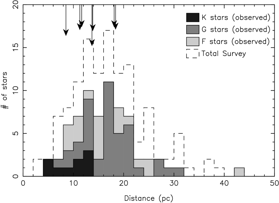
Figure 1: Distribution of stellar distances. Each spectral type is shaded with a different color, as indicated in the legend. The distances of stars found to have 70 µm excess (see §3.2) are flagged as arrows at the top of the plot. The length of the arrow is an indicator of the strength of 70 µm excess.

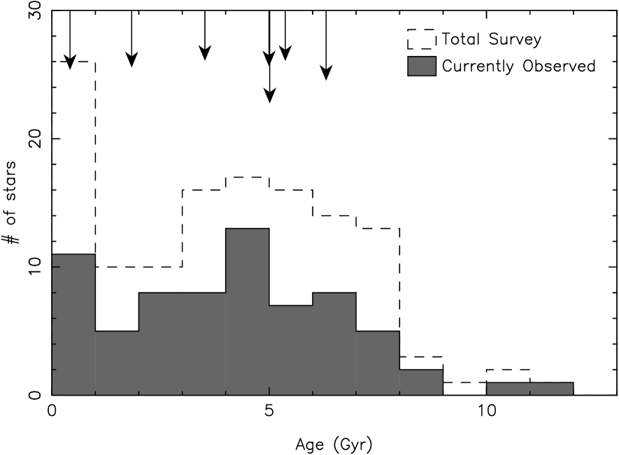
Figure 2: Distribution of stellar ages. The ages of stars with 70 µm excess are flagged as arrows at the top of the plot. The length of the arrow is an indicator of the strength of 70 µm excess. There is no strong correlation between the detection of an excess and the stellar age.

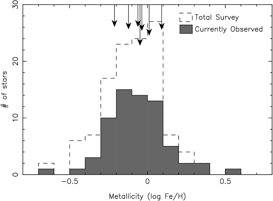
Figure 3: Distribution of stellar metallicities. The metallicities of stars with 70 µm excess are flagged as arrows at the top of the plot. The length of the arrow is an indicator of the strength of 70 µm excess. The detected excesses are distributed uniformly over the stellar metallicities.

The initial application of these criteria yields 131 stars. Of these, four are observed by other guaranteed-time programs (see Table Frequency of Debris Disks around Solar-Type Stars: First Results from a Spitzer/MIPS Survey). This leaves 127 total stars, 69 of which have currently been observed and are reported on here. Binned by spectral type, the sample contains 33 F5-F9 stars (20 observed), 46 G0-G4 stars (27 observed), 27 G5-G9 stars (13 observed), and 21 K0-K5 stars (9 observed). Among these stars are 15 with known planets, of which 11 have been observed. Typical distances range from 10 to 20 pc, closer for K stars and farther for earlier spectral types. Fig. 1 shows the distribution of stellar distances as a function of spectral type, with filled histograms for the currently observed stars and a dotted, open histogram for the eventual survey when complete. Some basic parameters of the sample stars are listed in Table Frequency of Debris Disks around Solar-Type Stars: First Results from a Spitzer/MIPS Survey, most importantly age and metallicity, which are also shown as histograms in Figs. 2 and 3.

3 Spitzer Observations

3.1 Data Reduction

Our data reduction is based on the DAT software developed by the MIPS instrument team (Gordon et al., 2005a). For consistency, we use the same analysis tools and calibration numbers as were adopted by Beichman et al. (2005a).

At 24 µm, we carried out aperture photometry on reduced images as described in Beichman et al. (2005a). At 70 µm we used images processed beyond the standard DAT software to correct for time-dependent transients, corrections which can significantly improve the sensitivity of the measurements (Gordon et al., 2005b). Because the accuracy of the 70 µm data is limited by background noise, rather than instrumental effects, a very small photometric aperture was used to maximize signal-to-noise – just 1.5 pixels in radius. With a 4 to 8 pixel radius sky annulus, this aperture size requires a relatively large aperture correction of 1.79. The flux level is calibrated at 15,800 $\mu$Jy/arcsec²/MIPS_70_unit, with a default color correction of 1.00 (MIPS_70_units are based on the ratio of the measured signal to the stimulator flash signal). Images were mosaiced from individual frames with half-pixel subsampling. For both the 24 µm and 70 µm data, neighboring point sources were subtracted from the images before measuring the sky brightness. With a telescope pointing accuracy of $<$1^′′ (Werner et al., 2004), the stars are well centered within the chosen apertures; no centroiding is required.

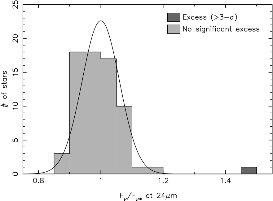
Figure 4: Distribution of 24 µm fluxes relative to the expected photospheric values. A Gaussian distribution with dispersion 0.06 is shown for comparison. One star (HD 69830) clearly stands out from the main population of stars which do not have significant excess emission above their stellar photospheres.

To determine whether any of our target stars have an IR excess, we compare the measured photometry to predicted photospheric levels (§A). After excluding one outlying point (HD 69830), the 69 flux measurements at 24 µm have an average $F_{\rm MIPS}/F_{\rm photosphere}$ of $0.99\,\pm\,0.01$; the agreement of the measured fluxes with prediction is not surprising given that the present Spitzer calibration is based on similar stellar models. More importantly for determining the presence of any excess, the dispersion of $F_{\rm MIPS}/F_{\rm photosphere}$ is 0.06 for this sample (see Fig. 4).

At 70 µm, 55 out of 69 stars are detected with signal-to-noise ratio $>3$. This is in contrast with previous IR surveys of A-K stars with ISO, in which only half of the stars without excess were detected (Habing et al., 2001). While the sensitivity of these Spitzer observations is roughly a factor of 10 better than previous data, Spitzer’s accuracy is limited by extragalactic source confusion and cirrus (see §3.2 below), which will make it difficult to look for weak excesses around stars much fainter than those discussed here.

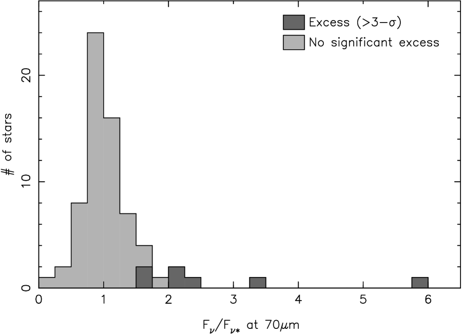
Figure 5: Distribution of 70 µm fluxes relative to the expected photospheric values. While most stars cluster around unity, where their flux is photospheric, several stars show a high degree of excess emission. Note that the distribution of excess stars is not completely continuous; whether a star has significant excess depends not only on the measured flux ratio $F_{\nu}/F_{\nu\star}$, but also on the level of background noise associated with each image.

The distribution of 70 µm flux densities relative to the expected photospheric values is shown in Fig. 5. Unlike the tight distribution of flux ratios at 24 µm, several stars have 70 µm flux density much higher than expected from the stellar photosphere alone. Seven stars, with 70 µm fluxes densities from 1.7 to 5.8 times the expected emission, are identified as having statistically significant IR excess (see below). Ignoring these stars with excesses and those with S/N $<3$, the average ratio of MIPS flux to predicted photosphere is $F_{\rm MIPS}/F_{\rm photosphere}=1.08\,\pm\,0.03$, consistent with the present calibration precision. The dispersion of $F_{\rm MIPS}/F_{\rm photosphere}$ relative to its mean is 25% in the 70 µm data (excluding the stars with excesses), considerably higher than that in the 24 µm data (6%). The following section discusses in more detail the noise levels within the 70 µm data.

Fig. 6 shows an illustrative spectral energy distribution for HD 166. Published photometric fluxes for this star from visible to infrared are well fit by a Kurucz stellar atmosphere (dotted line; Castelli, 2003; Kurucz, 2003). The Spitzer/MIPS 24 µm flux is also well fit by the model atmosphere, but the 70 µm emission is well above that expected from the stellar photosphere alone, requiring an additional component of emission due to dust. Because there is only a single 70 µm measurement of IR excess, however, the SED can be fit by a range of dust temperatures and luminosities. A methodology for constraining the dust properties in these systems is described in §4.

3.2 Analysis of Background Noise

An analysis of the noise levels in each field is required to assess whether the IR excesses are statistically significant. Many contributions to the overall error budget must be considered, including those arising from stellar photosphere modeling (§A), instrument calibration, sky background variation, and photon detector noise. For the 24 µm measurements, photon noise is negligible. Even with the minimum integration time (1 cycle of 3 sec exposures = 42 sec), the sensitivity of MIPS is overwhelming; our dimmest source could theoretically be detected in just a few milliseconds. Also, the background noise is low: galactic cirrus is weak at this wavelength, the zodiacal emission is relatively smooth across the field of view, and the confusion limit for distant extragalactic sources is just 0.056 mJy (Dole et al., 2004b).

Instead, for the 24 µm measurements, systematic errors dominate. The instrumental contribution to these errors is thought to be very low: 24 µm observations of bright calibrator stars are stable with 1% rms deviations over several months of observations (Rieke et al., 2004). However, for photometry of fainter stars, dark latent images of bright stars can result in larger errors because the star may be placed in a dip in the flat-fielded photometric image frame. In addition to any uncertainty in the instrument calibration, the dispersion in $F_{\rm MIPS}/F_{\rm photosphere}$ includes errors in the photosphere extrapolation as well as the effects of source variability. The fitting of the photosphere can be as precise as 2% when the best 2MASS $K_{s}$ band photometry is available (Skrutskie et al., 2000), but for stars brighter than $K_{s}\simeq 4$ mag, 2MASS data are less accurate and lower precision near-IR data and/or shorter wavelength observations must be relied upon. Extrapolation from visible data places considerably more weight on the photospheric models, increasing the uncertainty in the predicted photospheric levels at 24 µm and 70 µm. We expect that stellar photosphere fitting errors and flat field uncertainties due to latent images are the greatest contributors to the overall error budget. The net photometric accuracy is currently $\sim$6%, as seen in the dispersion in Fig. 4. Detections of excess at 24 µm (at the 3-$\sigma$ level) require measured fluxes at least 20% above the stellar photosphere (about 1000 times the Solar System’s 24 µm excess flux ratio).

While systematic errors dominate at 24 µm, for 70 µm data pixel-to-pixel sky variability becomes a major contributor to the overall uncertainty. This sky variation is a combination of detector/photon noise along with real fluctuations in the background flux. This background, a combination of galactic cirrus and extragalactic confusion, creates a noise floor that cannot be improved with increased integration time. To minimize this problem, the FGK target stars are chosen from areas of low galactic cirrus, as estimated from the IRAS Sky Survey Atlas (IPAC, 1994). The confusion limit for extragalactic background sources, however, is unavoidable and sets a strict lower limit for the sky noise at 70 µm.

We determine the pixel-to-pixel noise in each field by convolving the background image with the same top-hat aperture used for photometry (1.5 pixel radius) and then by calculating the dispersion within these background measurements. The region within 3 pixels of the target is excluded. The error on the mean noise is proportional to the square root of the number of contributing apertures. Based on this overall measured noise, we find the S/N for each star, as listed in Table 2. The median observed S/N for our target stars is $\sim$6, excluding the sources identified as having excess emission.

The measured noise (also listed in Table 2) can be compared to that expected from extragalactic confusion. Dole et al. (2004a, b) find a 5-$\sigma$ confusion limit of 3.2 mJy by extrapolating Spitzer source counts of bright objects down to fainter fluxes. In our sample, the lowest (1-$\sigma$) noise levels observed toward stars located in clean portions of the sky are $\sim$2 mJy, somewhat worse than Dole et al.’s best-case limit. This difference is attributable to the larger effective beam size used for our photometry/noise calculations, and to confusion noise in the limited sky area in our images. On top of the confusion limit, a few sources have higher noise values due to galactic cirrus and/or detector performance somewhat worse than typical.

The sky fluctuations in each field are a combination of detector noise plus real background variations. When the total observation can be separated into individual snapshots with shorter integration time (i.e. when there are multiple observing cycles), we can isolate the two sources of noise. We create several images at each integration time by separating the individual cycles and then adding chains of them together of various lengths. In each case, the noise is assumed to come from two terms added in quadrature, one constant and one declining with time. Specifically, the noise is fit to a function $\sqrt{B^{2}+(Dt_{\rm int}^{x})^{2}}$ where $B$ is the constant background, $D$ is the strength of the detector noise for 1 observing cycle, and $t_{\rm int}$ is the integration time (in cycles). Fig. 7 shows the resulting fit for HD 62613, a star observed for 10 cycles.

Naively, one would assume that detector noise drops off as the square root of integration time (i.e. $x=-1/2$). In practice, however, we find a typical time dependence of $x\simeq-0.6$. In other words, the noise drops off faster than expected. This surprising result follows from our method of data processing, which improves as more images are included in the analysis. The time-filtering routines have an optimal filtering window of 3-4 observing cycles (Gordon et al., 2005b), such that four cycles of integration time ($\simeq 400$ sec) result in less than half the detector noise of a single cycle ($\simeq 100$ sec).

Fig. 8 shows how the background in our MIPS data compares to IRAS-based predictions. For the single star with a very high level of cirrus contamination (HD168442, the rightmost point in Fig. 8), the IRAS noise level agrees well with that in the higher resolution MIPS field. Because the stars in this sample were pre-selected from regions of low cirrus contamination, however, the majority are not dominated by cirrus, and instead have background noise levels close to the extragalactic confusion limit. Note that the confusion limit here ($\sim$2 mJy) depends on our method of photometry (aperture size, shape, sky subtraction) and does not necessarily reflect the intrinsic properties of the instrument and the observed fields.

Finally, we consider any systematic errors. While we can directly examine the overall background noise in each of our 70 µm images, the systematic uncertainties are more difficult to evaluate. Repeated measurements of bright standards have rms scatter of $\sim$5%. The photospheric extrapolations may contribute 6% (judging from 24 µm). The detectors may also have a low level of uncorrected nonlinearity. We assume that the systematic errors in the 70 µm data are 15% of the stellar flux, about twice the dispersion in the 24 µm data.

Adding all of the noise sources (photon noise, sky background, model fitting, and residual calibration issues) together in quadrature gives us a final noise estimate for each 70 µm target. In Table 2 we list these noise levels, along with the measured and the photospheric fluxes, for each observed star. We use these noise estimates to calculate $\chi_{70}$, the statistical significance of any IR excess

$$\chi_{70}\equiv\frac{F_{70}-F_{\star}}{N_{70}}$$ (1)

where $F_{70}$ is the measured flux, $F_{\star}$ is the expected stellar flux, and $N_{70}$ is the noise level, all at 70 µm. Based on this criterion, we find that 7 out of 69 stars have a 3-$\sigma$ or greater excess at 70 µm: HD 166, HD 33262, HD 72905, HD 76151, HD 115617, HD 117176, and HD 206860. Of the remaining stars, 3-$\sigma$ upper limits on any excess flux vary from star to star, but are generally comparable to the stellar flux at 70 µm (the median upper limit is 0.8 $F_{\star}$).

While a strict 3-$\sigma$ cutoff is useful for identifying the stars most likely to have IR excess at 70 µm, several other stars below this limit may also harbor similar amounts of dust. HD 117043, for example, has a 70 µm flux density twice that expected from the stellar photosphere. A relatively dim source, this potential IR excess is not significant at the 3-$\sigma$ level ($\chi_{70}=2.4$), but is corroborated by a similarly high 24 µm flux (11% above photospheric). Similarly, Spitzer/IRS spectra can provide additional evidence for borderline cases. In all three cases where spectra have been obtained for stars with $>$3-$\sigma$ 70 µm excesses (HD 72905, HD 76151, and HD 206860) each spectrum contains clear evidence of a small excess at its longest wavelengths (from $\sim$25 to 35 µm; Beichman et al., 2006). Another star, HD 7570, with only 1.8-$\sigma$ significant excess at 70 µm, has a similar upturn in its spectra, suggesting that its moderately high level of 70 µm flux ($F_{\rm MIPS}/F_{\star}=1.5$) is in fact excess emission.

4 Properties of the Detected Dust

Our detections of IR excess provide only limited information about the properties of the dust in each system. In principle, each observed wavelength translates to a characteristic radial-dependent temperature and thus can tell us about a particular region of the dust disk. The exact location of dust at a given temperature depends on the stellar luminosity and on the grain emissivities. In general, though, dust in the inner system (${\buildrel<\over{\sim}}$  10 AU) has temperatures ${\buildrel>\over{\sim}}$  150 K and radiates strongly at 24 µm. The emission of dust at Kuiper Belt-like distances, with temperatures $\sim$50 K, peaks closer to 70 µm. For our 70 µm dust detections, the lack of 24 µm excess limits the amount of material in the inner system. In these cases, 24 µm measurements provide an upper limit on the dust temperature (as in Fig. 6), while sub-mm observations would set a lower limit. Because we usually have no information longward of 70 µm, however, only an upper limit on the temperature (or an inner limit on the dust’s orbital location) can be derived.

If a single dust temperature is assumed, the observed flux can be translated into the total dust disk luminosity relative to its parent star. For disks with detections of IR excess, a minimum dust luminosity can be calculated. On the Rayleigh-Jeans tail of the stellar blackbody curve, the ratio of dust to stellar fluxes is

$$\frac{F_{{\rm dust}}}{F_{\star}}=\frac{L_{\rm dust}}{L_{\star}}\;\frac{h\nu T_{\star}^{3}}{kT_{\rm dust}^{4}(e^{h\nu/kT_{\rm dust}}-1)}$$ (2)

The minimum disk luminosity as a function of 70 µm dust flux can be obtained by setting the emission peak at 70 µm (or, equivalently, $T_{\rm dust}=52.5$K) :

$$\frac{L_{\rm dust}}{L_{\star}}({\rm minimum})=10^{-5}\;\left(\frac{5600\;{\rm K}}{T_{\star}}\right)^{3}\;\frac{F_{70,{\rm dust}}}{F_{70,\star}}$$ (3)

Based on this equation, a minimum $L_{\rm dust}/L_{\star}$ is calculated for each of our target stars identified as having IR excess (see Table 2). The disk luminosity, however, could be greater than this value, depending on the dust temperature. In particular, a much larger amount of radiation could be emitted at unobserved sub-mm wavelengths. Fig. 9 shows the overall constraints on $L_{\rm dust}/L_{\star}$ as a function of $T_{\rm dust}$ for six stars identified as having excess 70 µm emission. The lines in this figure are 3-$\sigma$ limits to the observed 24 and 70 µm fluxes, while the filled, dark region corresponds to 1-$\sigma$ limits. The lack of excess emission at 24 µm excludes the upper right region of each plot (i.e. bright, hot emission) and typically constrains the dust temperature to be ${\buildrel<\over{\sim}}$  100 K at the 1-$\sigma$ level (solid-filled region).

Sub-mm observations are critical for constraining the dust properties beyond an upper bound for temperature and a lower limit for luminosity. For most of our stars with IR excess, large amounts of cold dust emitting at longer wavelengths cannot be ruled out. HD 72905, however, has been observed at 850 µm, with a measured flux of 1.1$\,\pm\,$1.2 mJy (Greaves et al., 2005a). Cold, very bright emission is excluded. Note that for the sub-mm flux, it is no longer appropriate to assume blackbody emission; as the wavelength of the emitted radiation becomes long compared to $2\pi a_{grain}$, the effective grain absorption cross-section begins to fall off as $\lambda^{-1}$ to $\lambda^{-2}$ (Draine & Lee, 1984; Wyatt & Dent, 2002). In order to calculate the most conservative limit on $L_{\rm dust}/L_{\star}$, we assume that the grains are small enough such that their emissivity drops off as $\lambda^{-2}$ for radiation longward of 100 µm. With the inclusion of this sub-mm limit, the dust temperature and luminosity for HD72905 are bounded by 1-$\sigma$ limits (solid-filled region in Fig. 9) of $T_{\rm dust}\approx 20$-100 K and $L_{\rm dust}/L_{\star}\approx 10^{-4.9}$-$10^{-4.1}$, i.e., within about a factor of six of the lower limit from 70$\mu$m data alone.

$T_{\rm dust}$ is meant to signify the typical emitting temperature for the dust; in reality some range of temperatures will be found in any given system. The approximate characteristics of the dust in the solar system, for example, have been included in Fig. 9, where the Kuiper and asteroid belts are shown as separate regions with discrete temperatures. There is growing evidence for multiple-component dust disks around other stars as well. Resolved images of the bright disk around Fomalhaut (Stapelfeldt et al., 2004) show that 24 and 70 µm emission can have markedly different spatial distributions. Observations of $\epsilon$ Eri’s disk (Megeath et al., 2005) similarly find 70 and 850 µm emission coming from completely distinct regions. For the unresolved sources considered here, the strong excess emission that we observe at 70 µm is clearly due to dust with colder temperatures than the asteroid belt, but a lower level of warm dust cannot be ruled out. In fact, follow-up IRS spectra suggest that small levels of warm dust orbiting inside of the dominant outer dust may be common in these systems (Beichman et al., 2006).

Even with full spectral and spatial coverage, it is difficult to determine the amount of dust responsible for the excess emission around these stars, let alone the overall mass of larger bodies that create the dust. Given the dust luminosity and temperature, the total cross-sectional area of the dust, $A_{d}$, is

$$A_{d}=\frac{\pi R_{\star}^{2}}{\epsilon_{\rm IR}}\,\frac{L_{\rm dust}}{L_{\star}}\,\frac{T_{\star}^{4}}{T_{\rm dust}^{4}}$$ (4)

where $\epsilon_{\rm IR}$ is the median grain emissivity over all wavelengths. For debris disks, this emissivity is observed to drop off as $\sim\lambda^{-1}$ at sub-mm wavelengths (Dent et al., 2000), consistent with the particle size distribution expected from a collisional cascade. In general, though, the magnitude of the grain emissivity is uncertain. Here, we assume that $\epsilon_{\rm IR}$ can be as high as unity if the dust is warm, but might be several orders of magnitude lower for cold dust. Even without this uncertainty in $\epsilon_{\rm IR}$, the dust area given by Eq. 4 is not well determined. Among our stars with IR excess, HD 72905 has the best constraints on disk brightness and temperature, yet the dust cross section can still range anywhere from $10^{24}$ to $10^{29}$ cm² (1-$\sigma$ limits). If the dust consists solely of micron-sized grains, this area corresponds to a dust mass of $\sim$10^-7-$10^{-2}M_{\oplus}$. The total mass of the debris disk, which tends to be dominated by the most massive objects, is even less well constrained. Under the assumption that the number of particles of a given size, ${r_{p}}$, follows the equilibrium size distribution $dn/d{r_{p}}\propto{r_{p}}^{-3.5}$ (e.g. Dohnanyi, 1968), the total mass can be estimated as a function of the largest planetesimal size, ${r_{\rm max}}$. For HD 72905, the disk mass is $\sim$10^-2-10³ $M_{\oplus}\sqrt{{r_{\rm max}}/10\,{\rm km}}$. The range of values in these mass estimates reflects the uncertainty in the dust location within these unresolved images (anywhere from $\sim$10 to 100’s of AU for the dominant component). The largest disks consistent with the SED observations can be ruled out by the lack of emission extended beyond the telescope PSF At HD 72905’s distance of 14.3 pc, a 300 AU diameter disk, subtending an angle of $\sim$2 instrument pixels, would be clearly extended in the 70 µm image. (The telescope’s FWHM at 70 µm is 18^′′.)

Although the dust temperature is generally not well determined by a single measurement of excess at 70 µm, the emission of HD 72905 in particular has been further constrained on the short end by IRS observations (Beichman et al., 2006). The upturn in the spectrum longward of $\sim$25 µm provides a very sensitive measure of the maximum dust temperature. From the combined spectral and photometric data, Beichman et al. (2006) estimate dust temperatures and masses for a variety of grain properties. For small 0.25 µm grains, they find dust temperatures ranging from 35 to 55 K, corresponding to a dust mass of $10^{-4}M_{\oplus}$, consistent with the above estimates.

For stars with no detected emission, 3-$\sigma$ upper bounds on the 70 µm fluxes lead to upper limits on $L_{\rm dust}/L_{\star}$ as low as as few times $10^{-6}$, assuming a dust temperature of $\sim$50 K (see Table 2). Although we cannot rule out cold dust at ${\buildrel>\over{\sim}}$  100 AU, we are placing constraints on dust at Kuiper Belt distances at $\sim$10-100 times the level of dust in our solar system. The constraint on asteroid belt-type dust is less stringent, at $\sim$1000 times our zodiacal emission. Many of our stars are bright ($>$30 mJy at 70 µm) and in regions of low background (a few mJy), such that the greatest source of error in their 70 µm flux is due to the overall calibration uncertainty of $\sim$15%. This uncertainty sets a threshold for minimum detectable $L_{\rm dust}/L_{\star}$ at $5\times 10^{-6}\,(T_{\star}/5600\,K)^{-3}$ (from Eq. 3).

5 Correlation of Excess with System Parameters

To understand the origin of any excess, we now consider the properties of the sample stars and how they correlate with excess detection. Specifically, we examine the correlation with three variables: 1) age, 2) metallicity, and 3) spectral type. These parameters are listed for each star in Table Frequency of Debris Disks around Solar-Type Stars: First Results from a Spitzer/MIPS Survey.

5.1 Age

Stellar youth is already well established as a primary indicator for excess IR emission (Spangler et al., 2001; Rieke et al., 2005). This connection is often interpreted as a continual decline in disk mass with time. Young stars lose their protostellar disks relatively quickly, transitioning from gaseous disks into less massive debris disks on time scales of $\sim$3 Myr (Haisch et al., 2001). While there is a correlation between stellar age and disk emission, the assumption that all debris disks gradually grind down into weak disks like the Sun’s is contradicted by observations of old stars with IR excess (Habing et al., 2001; Decin et al., 2000; Rieke et al., 2005). Strong collision events may be able to increase the dust emission, even at late times.

Unfortunately, there is no generally reliable age indicator for stars as old as those in our sample. Age estimates for our target stars generally span at least a factor of two, highlighting the difficulty in determining the ages of mature, main sequence stars. Whenever possible we adopt ages from the compilation of Wright et al. (2004), which provides a uniform tabulation for 1200 stars based on Ca II H&K line strengths. Otherwise an average of literature values is calculated. In addition to listing this age estimate for each of our target stars, Table Frequency of Debris Disks around Solar-Type Stars: First Results from a Spitzer/MIPS Survey also gives the maximum and minimum age found in the literature (for stars with more than one age estimate).

Fig. 2 shows the resultant histogram of stellar ages. Although our target selection criteria do not explicitly discriminate based on stellar age, young stars are not well represented in our sample due to their infrequent occurrence within $\sim$25 pc of the Sun. Therefore, our data cannot probe the rapid ($\sim$100 Myr) initial decline seen for samples of young stars, but instead are sensitive to any trends that occur over Gyr time scales.

The ages of the stars with excess are marked with arrows in Fig. 2. Most of the stars with excess are much older than a billion years; the one exception is HD 72905 which has a young age estimate (0.42 Gyr) based on its relatively high stellar activity. The average age of the stars with 70 µm excess is nearly identical to the average of the sample as a whole ($\sim$4 Gyr). We find no statistically significant correlation between age and excess.

5.2 Metallicity

The relationship of disk properties to the metallicity of the parent star is particularly important for understanding the formation and evolution of debris disks and, more generally, of larger planets. One might expect that the formation of objects composed of metals (i.e. dust, planetesimals, and terrestrial planets) will be strongly correlated with stellar metallicity. Gas giant planets, if their formation is preceded by the formation of a large solid core (e.g. Pollack et al., 1996), should also depend on the amount of solid material available in the protostellar disk. Alternately, if gas giants form via direct gravitational collapse of the disk (e.g. Boss, 2004), planet formation would only depend on metallicity through less important opacity effects.

In fact, there is a well known correlation between extrasolar gas giant planets and host star metallicity (Gonzalez, 1997; Santos et al., 2001). In particular, Fischer & Valenti (2005) find that the probability of harboring a radial-velocity detected planet increases as the square of the metallicity. However, there is as yet no evidence for a similar correlation between dust and metallicity. Greaves et al. (2005b) even find an anti-correlation between metallicity and dusty debris at sub-mm wavelengths. As an example, the $\sim$10 Gyr-old star $\tau$ Ceti has strong excess emission in both sub-mm (Greaves et al., 2004) and infrared wavelengths (Table Frequency of Debris Disks around Solar-Type Stars: First Results from a Spitzer/MIPS Survey), despite having only a third the metals of the Sun.

To look for any positive or negative correlation between metallicity and IR excess within our observed stars, we have collected metallicity data from the literature for our FGK targets. The majority of [Fe/H] values are derived from spectroscopic analysis; a few are from narrow-band filter photometry. While for some stars as many as seven independent values for [Fe/H] are available, no abundance information is available for five stars. Table Frequency of Debris Disks around Solar-Type Stars: First Results from a Spitzer/MIPS Survey lists the number of independent [Fe/H] estimates, their average, and the r.m.s. scatter for each star.

Fig. 3 shows a histogram of these metallicity values, which range from -0.5 to +0.5 dex with a mean value just below solar. The stars with IR excess are again identified with vertical arrows. In spite of any expectations, there is no evidence for higher metallicity resulting in a greater amount of IR emitting dust. The average [Fe/H] is -0.07$\,\pm\,$0.02 for the observed stars and -0.05$\,\pm\,$0.04 for the stars with excess – a small and insignificant difference. The correlation coefficient, $r$, between [Fe/H] and IR excess is 0.02$\,\pm\,$0.12. The strong type of relationship found between gas giant planets and metallicity would have resulted in a much stronger correlation ($r$=0.38$\,\pm\,$0.13) and can be confidently ruled out.

The lack of correlation between excess and metallicity is somewhat surprising given the strong correlation between planets and metallicity and the preliminary correlation that we have found between planets and excess (Beichman et al., 2005a). Our sample here, however, contains relatively few planet-bearing stars (11 out of 69). While these stars do have higher metallicity, only 1 out of 11 has an IR excess, resulting in a detection rate very similar to the non-planet stars and causing no net increase in the average metallicity of excess stars. If all of the planet-bearing stars described in Beichman et al. (2005a) are included within this sample, the correlation coefficient increases somewhat, but still not to a significant level.

While the lack of a metallicity-excess correlation may be surprising, there are several possible explanations. The formation of giant planets, which do have a strong metallicity correlation, requires a very massive protoplanetary disk. The disk that developed into the solar system, for example, originally contained more than $100M_{\oplus}$ of solid material, based on the composition of the planets today (Hayashi et al., 1985). Our Kuiper Belt is much smaller, currently containing only a few percent of $M_{\oplus}$ (Bernstein et al., 2004). In fact, very little mass is needed to produce the dust responsible for the observed IR excesses. Even disks with very small metallicity can easily contain the mass of planetesimals required to produce this dust.

A lower mass of solid material may even assist in dust production. Lower surface density disks contain less material for the largest growing bodies to accumulate. The amount of material that a solid core can directly sweep up (its isolation mass) increases as surface density to the 3/2 power (e.g. Pollack et al., 1996), such that disks with lower surface density tend to produce a larger quantity of smaller protoplanetary cores, rather than a few large planets. In this scenario, high metallicity would translate to larger planets and a cleaner, less dusty central disk. An outer fringe of smaller planetesimals, as in the solar system, could still form at or be scattered to the outer disk edge.

Another possibility is that there is an initial correlation between dust production and metallicity around young stars, but that this relationship disappears as the stars age. Dominik & Decin (2003) find that theoretical models of debris disk evolution tend to evolve toward the same final dust distributions over long enough time scales. While the more sparse disks (0.1 $M_{\oplus}$) evolve on Gyr time scales, the brightest disks generally decay relatively quickly. Disk models with initial masses ranging from 1 to 100 $M_{\oplus}$ converge toward the same asymptotic trend in less than a billion years, such that any initial differences in disk mass become unimportant for old systems. Star-to-star variability in dust emission may be strongly related to stochastic collisional events, rather than a simple function of initial disk mass.

5.3 Spectral Type

Within our observed range of spectral types ($T_{\star}\simeq 4500-6500$ K), we have not found any evidence for a correlation with excess emission. The average spectral type is G3 for both the stars with IR excess and for those without. The meaning of this flat trend is somewhat ambiguous based on our limited knowledge of the location of the dust, as well as the limited range of spectral types in our sample.

6 Frequency of IR Excess around Solar-Type Stars

The preliminary results of our survey contain enough excess detections at 70 µm to consider the overall statistics for emission by cold ($\sim$50 K) dust. Unlike previous investigations, we achieve photospheric detections at 70 µm for most of our sample, and the level of detectable disk brightness usually extends below $L_{\rm dust}/L_{\star}\sim 10^{-5}$. More importantly, our selection criteria produce an unbiased sample of observations that, combined with accurate knowledge of all measurement uncertainties, allow for a straightforward determination not only of the overall frequency of IR excess, but of the distribution of dust luminosities. Our sample is similar to a volume limited survey, rather than all-sky IRAS observations, which tend to pick out distant objects with strong excesses. Unlike a strict volume limited survey, however, we have maximized our detection efficiency by concentrating on the targets most likely to produce high signal-to-noise results.

The detection rate of IR excess depends both on the stellar emission and the achievable detection limits. From Eq. 3, the detection limit for each star is

$$\frac{L_{\rm dust}}{L_{\star}}({\rm detectable})=10^{-5}\;\left(\frac{5600\;{\rm K}}{T_{\star}}\right)^{3}\;\frac{3N_{70}}{F_{70,\star}}$$ (5)

where $N_{70}$ is the 1-$\sigma$ error in the flux measurement (listed in Table 2).

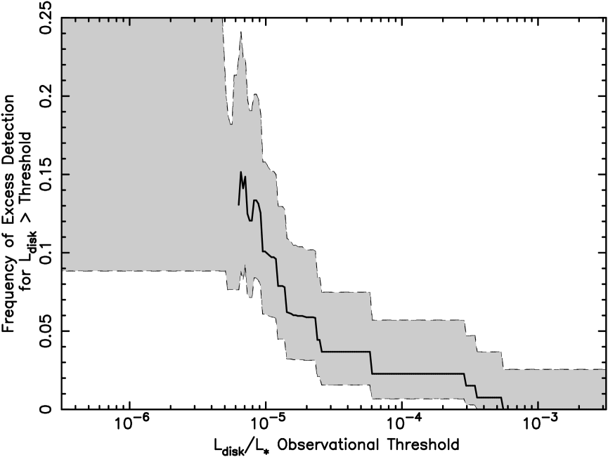
Figure 10: The frequency of 70 µm excess detection as a function of the observational threshold in terms of $L_{\rm dust}/L_{\star}$. In addition to the 69 observed stars, a few stars reserved by other programs (Table Frequency of Debris Disks around Solar-Type Stars: First Results from a Spitzer/MIPS Survey) have been included in the figure with appropriate weighting. Even including these bright IRAS sources, above $L_{\rm dust}/L_{\star}\simeq 10^{-3}$ there are no detections. The gray region indicates the 1-$\sigma$ limits to the distribution based on proper binomial statistics. The lack of sensitivity below $5\times 10^{-6}$ is reflected in the large unconstrained gray region filling the upper-left section of the plot.

Fig. 10 shows how frequently we detect debris disks above a range of detection thresholds. For each observational threshold (each $L_{\rm dust}/L_{\star}$), only stars with a lower detectability limit (Eq. 5) are considered. The 70 µm observations are generally very sensitive to disks with $L_{\rm dust}/L_{\star}>10^{-5}$, with many cleaner fields sensitive to as low as $\sim 5\!\times\!10^{-6}$. Below this level, we have no direct measurements of the disk frequency, and the 1-$\sigma$ constraints on the frequency of excess detection (the shaded region in the figure) are not well defined.

As discussed in §2, 131 stars meet our selection criteria for an unbiased sample. However, four of these are well-known IR-excess sources that have been reserved by other programs (Table Frequency of Debris Disks around Solar-Type Stars: First Results from a Spitzer/MIPS Survey). To avoid a bias against strong excesses, these stars have also been included into the overall statistics of Fig. 10, with weighting appropriate for the fraction of stars currently observed (69/127).

Even with the inclusion of these bright disks, we find that the frequency of disk detection increases steeply as the detection limit is extended down to dimmer disks. While debris disks with $L_{\rm dust}/L_{\star}\sim 10^{-3}$ are rare around old solar-type stars, the disk frequency increases from 2$\,\pm\,$2% for disks with $L_{\rm dust}/L_{\star}>10^{-4}$ to 12$\,\pm\,$5% for $L_{\rm dust}/L_{\star}>10^{-5}$. Our overall detection rate is in good agreement with the results of Kim et al. (2005), who find five 70 µm excesses in a sample of 35 solar-type stars, a detection rate of $14\pm 6\%$.

With these data, we can start to place the dusty debris in the solar system into context relative to other solar-type stars. Extrasolar planetary systems with architectures very different from our own continue to be discovered. With highly eccentric planets, short-period planets, and resonantly locked planets all commonly seen around other stars, the solar system may not be a typical planetary system, nor may its interplanetary dust be typical.

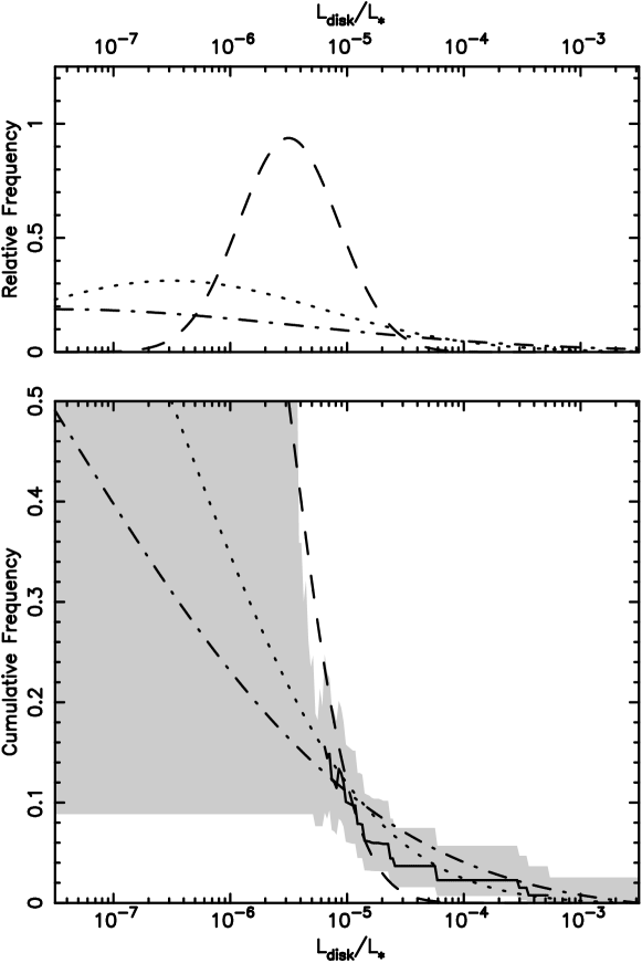
Figure 11: Disk detection frequency compared with theoretical debris disk distributions. Three possibilities are considered: 1) all stars have disks, with the solar system’s level of emission ($\sim 10^{-6.5}$) as average (dotted), 2) all stars have disks with average 10 times solar (dashed), and 3) all stars have disks with average 10 times less than solar (dot-dash). The relative frequencies of disk luminosity (upper panel) are assumed to follow Gaussian distributions, with the cumulative frequency of disks with $L_{\rm dust}/L_{\star}>10^{-5}$ fixed at 12% in each case. The corresponding cumulative frequency distributions are shown in the lower panel. The detection frequency within our data is plotted as a solid line for comparison. As in Fig. 10, the region constrained by our observations is shown in gray (1-$\sigma$). Of the three curves, the distribution with solar as average (dotted) is the best fit to the data.

Fig. 11 shows our observed 70 µm disk brightness distribution compared with several simple theoretical distributions. Three possibilities for the median disk luminosity are considered: equal to the Kuiper Belt’s level of emission ($\sim$$10^{-6.5}$, dotted), ten times above this level (dashed), and ten times below (dot-dash). In each case, we set the frequency of disks with $L_{\rm dust}/L_{\star}\ \lower 3.0pt\hbox{${\buildrel>\over{\sim}}$}\ 10^{-5}$ at 12%, in accordance with Fig. 10. Also, we assume Gaussian distributions of disk luminosities (in logarithmic space), resulting in standard deviations of 1.8, 3.0, and 0.6 decades for the three curves. The true distribution of disk luminosities is not a strict Gaussian, but more likely has an extended tail of strong emitters resulting from recent collisional events. Nonetheless, under the rough assumption that the distribution of debris disk luminosities follows a Gaussian-shaped profile, our existing dataset can already limit the theoretical disk distributions to some extent. In particular, the possibility that most stars have disks much brighter than the solar system’s (dashed lines) appears to be inconsistent with the constraints provided by our observations (gray region).

7 Summary

We have searched for circumstellar dust around an unbiased sampling of 69 F5-K5 stars by means of photometric measurements at 24 µm and 70 µm. We detected all the stars at 24 µm with high S/N and 80% of the stars at 70 µm with S/N $>3$. Uncertainties in the Spitzer calibration and in the extrapolation of stellar photospheres to far-IR wavelengths limit our ability to detect IR excesses with 3-$\sigma$ confidence to $\sim$20% and $\sim$50% of the photospheric levels at 24 and 70 µm, respectively.

Of the 69 stars, we have a single detection of excess at 24 µm, for an overall detection rate of $\sim$1%. At 70 µm, seven stars show significant excesses ($>$3-$\sigma$). When we correct the detection statistics for large-excess stars intentionally left out of the sample, the incidence of 70 µm excesses in this type of star is $13\pm 5$%. With only a single wavelength of excess measurement, the dust properties for these stars are not well constrained, but are generally consistent with Kuiper Belt configurations – distances from the star of several tens of AU and temperatures of $\sim$50 K. The observed dust luminosities, however, are much brighter than in the solar system, generally exceeding the Kuiper Belt’s $L_{\rm dust}/L_{\star}$ by factors of $\sim$100.

Cross-correlating the detections of IR excess with stellar parameters we find no significant correlations in the incidence of excesses with 1) age, 2) metallicity, or 3) spectral type. The restricted range of the sample in age and spectral type may hide more global correlations that can be explored with broader samples. The lack of correlation with metallicity contrasts with the known correlation between planet detections and stellar metallicity, and the expectation that higher metal content might result in a greater number of dust-producing planetesimals.

We have a large enough sample of excess detections at 70 µm to fit the cumulative distribution, which rises from $\sim$2% for $L_{\rm dust}/L_{\star}>10^{-4}$ to $\sim$12% for $L_{\rm dust}/L_{\star}>10^{-5}$. Under the assumption that the distribution of disk luminosities follows a Gaussian distribution, the current observations suggest that the infrared emission by dust in the Kuiper Belt must be within a factor of 10, greater or less, of the typical level for an average solar-type star.

While only one star has detectable excess emission at 24 µm (HD69830; see Beichman et al., 2005b), in some ways we are less sensitive to dust at that wavelength. Although better instrumentation gives us better sensitivity at 24 µm in terms of the relative flux ($F_{\rm dust}/F_{\star}$), as far as fractional disk luminosity we are only sensitive to disks with $L_{\rm dust}\lower 3.0pt\hbox{${\buildrel>\over{\sim}}$}\ 5\!\times\!10^{-5}\,L_{\star}$ at 24 µm, an order of magnitude worse than at 70 µm. This detection threshold is many orders of magnitude above the luminosity of the asteroid belt ($L_{\rm dust}/L_{\star}\simeq 10^{-8}$-$10^{-7}$; Dermott et al., 2002). The disks that we are detecting have typical 70 µm luminosities around 100 times that of the Kuiper Belt. If they also have inner asteroid belts 100 times brighter than our own, we would still not be able to detect the warm inner dust. In other words, the observed 70 µm excess systems could all be scaled-up replicas of the solar system’s dust disk architecture, differing only in overall magnitude. These systems could have planets, asteroids, and Kuiper Belt Objects as in our own system, but simply with a temporarily greater amount of dust due to a recent collisional event.

Appendix A Modeling the Stellar Photosphere

Developing accurate spectral models for the photospheres of our target stars is critical for determining the presence and strength of any IR excess. This is particularly true for measurements with low background noise (i.e. 24 µm) where inaccuracy in our photospheric models is likely to be the greatest source of uncertainty in identifying excess emission. Accordingly, we have compiled the best available photometric measurements for our target stars and used this data to extrapolate from visible/near-IR wavelengths out to 24 and 70 µm. Fortunately, the FGK sample is made up of bright, well-known stars of solar-like spectral types, making the photospheric modeling relatively straightforward.

From the literature we have assembled visible photometry in five bands: $U$, $B$, $V$, $R$, and $I$. Whenever possible, we derived B and V data from the Hipparcos satellite measurements (ESA, 1997) transformed to a common Johnson color system. These Hipparchos magnitudes are typically accurate to $\sim$0.01 mag. Data at $U$, $R$, and $I$ come from a wide variety of references, including compilations by Johnson & Mitchell (1975), Morel & Magnenat (1978), Bessel (1990), Guarinos (1995), de Geus et al. (1994), and Bessel (1990). Five near-IR bands ($J$, $H$, $K$/$K_{s}$, $L$/$L^{\prime}$, and $M$) are considered; data in these bands come from the visible photometry references, from data compiled in Gezari et al. (1993, 1999), and from the 2MASS catalog. For stars with high quality detections, IRAS measurements at 12 and 25 µm are also included; fluxes from the IRAS Faint Source Catalog (Moshir et al., 1990) have been color corrected based on the stellar effective temperature. For most of our sources, 2MASS photometry sets a limiting accuracy of $\sim$2% in our extrapolation to MIPS wavelengths. Many stars, however, are bright enough ($K_{s}\lower 3.0pt\hbox{${\buildrel<\over{\sim}}$}\ 4$) to saturate one or all of the 2MASS bands. 2MASS accuracy in these cases is only 0.10-0.25 mag, such that the Hipparcos visible photometry plays a greater role in the overall fit.

The compiled data is fit with Kurucz stellar atmosphere models (Kurucz, 1992; Lejeune et al., 1997; Castelli, 2003; Kurucz, 2003), which are appropriate for the F-K type stars considered here. Each Kurucz model was integrated over representative filter and atmospheric passbands, incorporating the effects of spectral lines that are particularly important in the $U$, $B$, and $V$ bands. The Johnson system flux zero points are taken from Campins et al. (1985) and Rieke et al. (1985). Flux uncertainties for each photometry band are taken as their published errors, but with an imposed minimum fractional uncertainty of 2%.

In addition to the photometric fluxes, each star’s observed spectral type and metallicity ($[Fe/H]$) are given as inputs to the program, with assumed errors of 250 K for $T_{eff}$ and 0.25 dex for $[Fe/H]$. The fitting program steps through a discrete grid of effective temperatures spaced every 250 K and [Fe/H] values of -1.0, -0.5, -0.2, 0.0, 0.2, 0.5, and 1.0. While the logarithm of the stellar surface gravity, $\log{g}$, is known to vary from 4.32 to 4.60 for F5 to K5 stars (Gray, 1992), we assume $\log{g}$ = 4.5 for all cases. A microturbulent velocity of 2.00 km s^-1 is also assumed.

Given the uncertainties for each variable, a minimum-$\chi^{2}$ fit is obtained, scaling the data to Kurucz-Lejeune models. For each wavelength, the r.m.s. dispersion in the fits is very similar to the input uncertainties, as desired. While the average observed fluxes at each wavelength ($1/\sigma^{2}$-weighted, with rejection of 2-$\sigma$ outliers) are typically within a few percent of the model values, some bands stand out above this typical $\sim$2% offset. At $U$, for example, the data consistently lie an average of 4.7% below the models. Given the difficulty both in calibrating $U$ band photometry and in computing $U$ band model photospheres, the large errors at this wavelength are not unexpected. There is also a fitting offset at 25 µm, where the IRAS data sit 4.7% above the models, an apparent excess that has been attributed by a number of authors to a small miscalibration of the IRAS data at 25 µm (e.g. Cohen et al., 1999). With the exception of $U$ band and 25 µm data, the reasonableness of the fits is good within the prescribed errors. The average offset, combining all wavelengths, is just -0.2%.

Figure 6: Spectral energy distribution for HD 166. In addition to our 24 and 70 µm Spitzer data (dark circles), we also show optical, near-IR, and IRAS fluxes from the literature (error bars), which are well fit by a stellar Kurucz model (dotted line). Two possible dust temperatures are considered in order to fit the 70 µm excess emission - 50 and 300 K (dashed lines). Only the cold, 50 K dust is consistent with the observed 24 µm flux; hotter, 300 K dust is ruled out as the dominant source of IR excess.

Figure 7: 70 µm background noise as a function of MIPS integration time for the field surrounding HD 62613. Measurements within the MIPS frames from 1 to 10 cycles (crosses) are fit by a combination of detector noise (dotted) and underlying background (dashed). While photon detector noise decreases with integration time, the background, a combination of galactic cirrus and extragalactic confusion, does not.

Figure 8: Measured background noise level within 70 µm MIPS images compared with the estimated cirrus background based on IRAS data. The MIPS noise here is from background only; detector noise has been subtracted to the extent given by the error bars. Only shown are those stars with enough images (at least 4 observing cycles) to disentangle the detector noise from the real sky background. The overall trend of the noise is well fit by the IRAS estimate for galactic cirrus (dashed line) combined with a $\sim$2 mJy lower limit from extragalactic confusion (dotted).

Figure 9: Constraints on the temperature and total luminosity of the dust around six stars with 70 µm excess emission. The upper right of each panel (bright, hot emission) is ruled out by the 24 µm upper limits. For HD 72905 (upper right panel) the upper left of the plot (bright, cold emission) is also ruled out by sub-mm observations (Greaves et al., 2005a). Based on the measured 70 µm excess, possible dust temperatures and luminosities are shown as shaded regions (cross-hatched for 3-$\sigma$ error limits; solid-filled for 1-$\sigma$ limits). The approximate characteristics of the asteroid and Kuiper belts are shown for comparison.

Table 1: FGK Survey Stars

Star	Spectral	V		Age (Gyr)				[Fe/H]
	Type	(mag)	Wr/Averagec	Min	Max	Refs	Average	Dispersion	# est.	Refs
HD 166a	K0 Ve	6.16	5.0	0.04	5.0	Wr,Ba	-0.05	0.15	5	Ca,E,M,Hy,Ga
HD 1237a,b	G6 V	6.67	2.8	0.6	2.8	Wr,L	0.1	0.08	5	Ca,B,Hy,Go,Ga
HD 1581a	F9 V	4.29	3.0	3.0	10.7	Wr,L	-0.23	0.1	8	T,Ca,E,M,Hy,L
HD 4628a	K2 V	5.85	8.1	5.5	11.0	L	-0.22	0.11	6	E,Ca,M,Ce,L
HD 7570a	F8 V	5.03	4.3	1.1	7.8	M,F,L	0.04	0.1	5	T,Ca,M,E,L
HD 10800a	G2 V	5.95	7.4	-	-	F	-0.03	0.08	2	M
HD 13445a,b	K1 V	6.21	5.6	3.7	7.6	L	-0.19	0.04	5	Ca,E,B,M,Hy
HD 17051a,b	G0 V	5.46	2.4	0.5	5.1	M,B,L,Lw	0.09	0.11	6	Ca,M,E,B,Gi,L
HD 20766a	G2 V	5.57	5.2	2.9	7.9	L	-0.2	0.07	7	T,Ca,E,Hy,L
HD 33262a	F7 V	4.77	3.5	1.2	6.5	L	-0.21	0.07	5	T,Ca,M,E,L
HD 34411a	G1.5IV-V	4.76	6.8	4.6	9.4	Wr,M,Ba,L	0.05	0.07	6	T,Ca,M,L,Bo,B
HD 35296a	F8 Ve	5.06	3.8	0.02	7.5	C,Ba	-0.06	0.09	4	T,Ca,M,C
HD 37394a	K1 Ve	6.30	0.5	0.3	0.9	L	-0.07	0.1	7	T,Ca,E,Hy,L,Le,Ga
HD 39091a,b	G1 V	5.72	5.6	3.9	7.3	M,F	0.11	0.11	5	T,M,E,Ca,Hy
HD 43162a	G5 V	6.45	0.4	-	-	Wr	-0.14	0.04	2	Hy,Ga
HD 43834a	G6 V	5.15	7.6	5.1	10.5	L	0.04	0.12	7	T,Ca,E,M,Hy,L
HD 50692a	G0 V	5.82	4.5	-	-	Wr	-0.19	0.11	2	M,E
HD 52711a	G4 V	6.00	4.8	4.8	6.4	Wr,Ba	-0.16	0.03	4	T,Ca,M,E
HD 55575a	G0 V	5.61	4.6	4.6	10.6	Wr,C	-0.3	0.08	6	T,Ca,M,C,E,Bo
HD 58855a	F6 V	5.41	3.6	-	-	C	-0.27	0.08	5	T,Ca,M,C,Ms
HD 62613a	G8 V	6.63	3.1	3.1	5.2	Wr,Ba	-0.17	0.04	2	E,Hy
HD 68456a	F5 V	4.80	2.4	-	-	M	-0.28	0.07	4	T,Ca,M,E
HD 69830a	K0 V	6.04	4.7	0.6	4.7	Wr,So	0.0	0.06	4	Ca,E,Hy,M
HD 71148a	G5 V	6.39	4.7	4.7	5.6	Wr,Ba	-0.05	0.18	3	M,E,Hy
HD 72905a	G1.5 V	5.71	0.4	0.01	0.4	Wr,Ba,W	-0.04	0.1	5	T,Ca,M,E,Ga
HD 75732a,b	G8 V	6.04	6.5	3.6	6.5	Wr,B,Lw	0.31	0.13	7	T,Ca,B,M,Hy,Ce
HD 76151a	G3 V	6.08	1.8	0.8	4.1	M,L	0.09	0.05	5	T,Ca,M,E,L
HD 84117a	G0 V	4.98	4.2	2.5	6.0	M,F	-0.15	0.07	4	T,M,E,Hy
HD 84737a	G0.5 Va	5.16	11.7	4.3	11.7	Wr,M,F,Ba,L	0.04	0.04	5	T,Ca,M,E,L
HD 88230a	K2 Ve	6.75	4.7	-	-	L	-0.02	0.61	4	Ca,Ce,B,Ma
HD 90839a	F8 V	4.88	3.4	0.2	5.2	Wr,C,Ba,L	-0.15	0.07	5	T,Ca,M,C,L
HD 95128a,b	G0 V	5.1	6.0	3.9	8.3	Wr,B,Ba,L,Lw	-0.01	0.05	7	T,Ca,M,C,Gi,L,Lw
HD 101501a	G8 Ve	5.39	1.1	0.5	2.5	Wr,Ba,L	-0.2	0.21	8	T,Ca,E,M,Ce,Hy,L
HD 102870a	F9 V	3.66	4.5	2.2	7.5	Wr,M,Ba,L	0.14	0.06	7	T,Ca,M,C,L,Bo,B
HD 114710a	F9.5 V	4.31	2.3	1.8	9.6	Wr,C,Ba,L	0.03	0.07	8	T,Ca,M,C,Ms,L,Le,Bo
HD 115383a	G0 V	5.26	0.4	0.1	5.7	Wr,M,C,Ba,L	0.02	0.06	8	Hy,M,C,Ca,L
HD 115617a	G5 V	4.81	6.3	4.4	9.6	Wr,L	0.01	0.04	5	T,Ca,E,L,Bo
HD 117043a	G6	6.58	-	-	-	-	0.22	-	1	Hy
HD 117176a,b	G2.5 Va	5.05	5.4	5.4	12.1	Wr,B,Ba,L,Lw	-0.06	0.04	9	T,Ca,B,M,Ce,Ms,Gi,Lw
HD 122862a	G2.5 IV	6.08	6.1	4.8	7.4	M,F	-0.16	0.05	3	M,F,E
HD 126660a	F7 V	4.10	2.8	0.4	4.7	M,Ba,L	-0.11	0.11	6	T,Ca,M,Ce,L
HD 130948a	G2 V	5.94	0.9	0.9	10	Wr,C,W	-0.02	0.14	6	Ca,M,C,E,Ga,B
HD 133002a	F9 V	5.71	2.5	-	-	F	-	-	0	-
HD 134083a	F5 V	4.98	1.7	0.9	2.5	L	-0.01	0.09	5	T,Ca,M,E,L
HD 136064a	F8 V	5.21	4.6	4.5	4.8	M,F	-0.04	0.02	7	T,Ca,M
HD 142373a	F9 V	4.67	8.1	7.1	9.7	Wr,M,C,Ba,L	-0.45	0.07	7	T,Ca,M,C,Ms,L,Bo
HD 142860a	F6 IV	3.88	2.9	2.4	4.3	Wr,C,L	-0.16	0.08	8	T,Ca,C,M,L
HD 143761a,b	G0 V	5.47	7.4	7.4	12.1	Wr,M,C,B,Ba,Lw	-0.23	0.05	6	T,Ca,M,C,Gi,Bo
HD 146233a	G1 V	5.56	4.6	4.4	4.6	Wr,M	0.06	0.04	4	T,Ca,M,E
HD 149661a	K2 V	5.86	1.2	1.2	3.1	Wr,L	0.11	0.26	6	E,Ca,M,Hy,Ce,L
HD 152391a	G8 V	6.74	0.6	0.3	0.6	Wr,Ba	-0.11	0.07	4	E,M,Hy,Ga
HD 157214a	G2 V	5.46	6.5	5.6	12.0	Wr,Ba,L	-0.36	0.04	8	T,Ca,M,Hy,Ce,Ms,L
HD 166620a	K2 V	6.49	5.0	4.4	12.0	Wr,L	-0.18	0.14	7	T,E,Ca,Ce,Hy,L,Le
HD 168151a	F5 V	5.04	2.5	2.4	2.7	M,C,F	-0.28	0.08	4	T,Ca,M,C
HD 173667a	F6 V	4.26	3.4	2.1	3.8	Wr,M,L	-0.12	0.05	4	T,Ca,M,L
HD 181321a	G5 V	6.55	0.5	-	-	W	-	-	0	-
HD 185144a	K0 V	4.76	3.2	3.2	6.9	Wr,Ba,L	-0.23	0.13	6	T,E,Ca,M,L,Le
HD 186408a	G1.5 Vb	5.96	10.4	-	-	N	0.08	0.10	3	T,Ca
HD 186427a,b	G3 V	6.29	8.7	8.3	9.1	B,Lw	0.06	0.04	6	T,Ca,E,B,Gi,Bo
HD 188376a	G5 V	4.77	7.4	-	-	Wr	-0.02	0.15	2	T,Ca
HD 189567a	G2 V	6.15	4.5	-	-	Wr	-0.26	0.07	6	T,Ca,E,M,Hy
HD 190248a	G7 IV	3.62	5.3	-	-	L	0.36	0.11	6	T,Ca,E,M,Hy
HD 196378a	F8 V	5.18	6	5.8	6.2	M,F	-0.39	0.06	3	T,Ca,M
HD 197692a	F5 V	4.19	1.9	1.4	2.5	L	0.0	0.06	6	T,Ca,M,L
HD 203608a	F8 V	4.28	10.2	6.5	14.5	C,F,L	-0.65	0.11	5	T,Ca,M,C,L
HD 206860a	G0 V	6.02	5.0	0.09	9.9	C,Ba	-0.12	0.08	5	Ca,M,C,E,Ga
HD 210277a,b	G0V	6.63	6.8	6.8	6.9	Wr,B,Lw,L	0.23	0.01	3	Ca,B,Hy
HD 216437a,b	G2.5IV	6.13	7.2	6.3	8.0	F,R	0.2	0.1	4	M,Ca,R
HD 221420a	G2 V	5.89	5.5	-	-	F	0.55	-	1	M
HD 693	F5 V	4.95	5.2	4.3	5.9	M,C,L	-0.4	0.03	5	T,Ca,M,C,L
HD 3302	F6 V	5.56	7.8	2.1	7.8	Wr,M,F	-0.23	0.29	2	M,E
HD 3651b	K0 V	5.97	5.9	-	-	Wr	-0.03	0.1	5	T,Ce,E,Ca,M
HD 3795	G3 V	6.23	7.2	7.2	10.8	Wr,F	-0.67	0.04	4	Ca,Ms
HD 3823	G1 V	5.96	5.5	4.9	10.5	Wr,M,F	-0.32	0.1	4	Ca,M,E
HD 4307	G2 V	6.22	7.8	7.2	7.8	Wr,M	-0.24	0.04	5	T,Ca,M,E,Bo
HD 9826b	F8 V	4.16	6.3	2.3	6.3	Wr,M,B,Ba,L,Lw	0.04	0.07	6	T,Ca,M,C,Gi,L
HD 10476	K1 V	5.34	4.6	-	-	Wr	-0.16	0.05	6	T,Ca,E,Ce,M,Le
HD 10697b	G5 IV	6.36	7.4	7.4	7.9	Wr,F,Lw	0.1	0.08	5	Ca,B,Ms,Go,Gi
HD 13555	F5 V	5.28	2.7	2.7	2.8	C,F	-0.3	0.05	4	T,Ca,M,C
HD 14412	G5 V	6.42	3.3	3.3	12	Wr,L	-0.42	0.66	4	Ca,E,Hy,L
HD 14802	G2 V	5.27	6.8	5.0	6.8	Wr,M,L	-0.09	0.04	6	Ca,M,E,Ce,L
HD 15335	G0 V	5.97	7.8	6.9	8.1	Wr,M,C,F	-0.21	0.04	4	T,Ca,M,C
HD 15798	F5 V	4.79	3.2	2.5	4.1	M,C,F	-0.25	0.02	4	T,Ca,M,C
HD 16160	K3 V	5.80	-	-	-	-	-0.08	0.04	3	E,Hy,Ce
HD 17925	K1 V	6.15	0.2	0.04	0.5	L,W	-0.02	0.11	7	T,Ca,E,M,Hy,L,Le
HD 19373	G0 V	4.12	5.9	2.1	8.1	Wr,C,Ba,L	0.09	0.08	6	T,Ca,C,E,L,Bo
HD 20630	G5 Ve	4.92	0.3	0.2	0.4	Ba,L	0.0	0.09	8	T,Ca,E,M,Mu,Ce,L
HD 20807	G1 V	5.30	7.9	4.4	12	L	-0.2	0.04	8	T,Ca,E,M,Hy,L
HD 22484	F8 V	4.36	8.3	4.6	8.4	Wr,C,M,Ba,L	-0.11	0.06	6	T,Ca,M,C,L,Bo
HD 26923	G0 IV	6.38	-	-	-	-	0.0	0.06	5	Ca,M,R,Ga
HD 30495	G1 V	5.56	1.3	0.2	1.3	Wr,L	0.0	0.08	6	Ca,M,E,Hy,L,Ga
HD 30652	F6 V	3.24	1.5	-	-	Wr	0.0	0.06	6	T,M,E,Ca,Ce
HD 33564	F6 V	5.14	3.5	-	-	M	-0.12	0.01	2	M,E
HD 34721	G0 V	6.02	6.2	3.8	6.2	Wr,M	-0.13	0.09	5	Ca,M,E,Hy
HD 69897	F6 V	5.18	3.5	1.9	4.7	Wr,C,L	-0.26	0.04	5	T,Ca,M,C,L
HD 86728	G3 Va	5.45	6.9	1.5	6.9	Wr,F	0.0	-	1	M
HD 94388	F6 V	5.29	3.2	-	-	M	0.09	0.06	3	T,Ca,M
HD 102438	G5 V	6.56	-	-	-	-	-0.21	0.26	3	E,Hy,M
HD 103932	K5 V	7.10	-	-	-	-	0.16	-	1	Ca
HD 104731	F6 V	5.21	1.8	1.7	2	M,F	-0.15	0.05	3	Ca,M
HD 110897	G0 V	6.02	9.7	4.9	14.5	C,Ca	-0.49	0.06	5	T,Ca,M,C,Bo
HD 111395	G7 V	6.37	1.2	-	-	Wr	0.07	0.1	3	E,M,Hy
HD 112164	G1 V	5.96	3.4	3.2	3.6	M,F	0.25	0.1	4	T,Ca,M
HD 114613	G3 V	4.93	5.3	-	-	F	-	-	0	-
HD 118972	K1	7.02	-	-	-	-	-0.05	-	1	Ga
HD 120690	G5 V	6.52	2.2	-	-	Wr	-0.1	0.02	3	Ca,E,Hy
HD 127334	G5 V	6.44	6.9	6.9	15.9	Wr,C	0.11	0.04	4	T,Ca,C,E
HD 131156	G8 V	4.55	-	-	-	-	-0.01	0.23	4	Ca
HD 154088	G8IV-V	6.68	5.9	4.4	12.0	Wr,L	0.29	0.01	2	Hy,M
HD 181655	G8 V	6.36	4.6	4.6	11.1	Wr,F	0.05	-	1	E
HD 190007	K4 V	7.60	-	-	-	-	-	-	0	-
HD 191408	K3 V	5.41	7.9	4.4	12.0	L	-0.4	0.12	6	T,Ca,E,Hy,L
HD 193664	G3 V	5.98	4.7	4.7	4.7	M,Ba	-0.1	0.09	6	T,M,E,Hy,Ca
HD 196761	G8 V	6.44	4.3	-	-	Wr	-0.43	0.24	2	E,Hy
HD 207129	G0 V	5.64	5.8	4.3	8.3	M,L	-0.08	0.04	5	Ca,M,E,L
HD 209100	K5 Ve	4.83	1.4	0.8	2.0	L	0.01	0.1	3	Ca,M,L
HD 210302	F6 V	4.99	5.4	2.5	5.4	Wr,M	0.05	0.11	4	T,Ca,M,E
HD 210918	G5 V	6.29	3.9	-	-	M	-0.1	0.14	6	Ca,E,M,Hy
HD 212330	G3 IV	5.40	7.9	-	-	R	-0.04	0.09	6	T,Ca,Hy,R
HD 216803	K4 V	6.60	-	-	-	-	0.08	0.01	2	Sa,M
HD 217014b	G4 V	5.52	7.4	4.4	10.0	Wr,B,Ba,L,Lw	0.17	0.03	8	T,Ca,E,B,Go,Gi,L
HD 217813	G5	6.73	0.7	0.7	5.6	Wr,M	-0.02	0.07	4	M,Hy,Ga
HD 219134	K3 V	5.67	12.6	-	-	L	0.05	0.14	8	T,E,Ca,Mu,Hy,Ce,Le,Bo
HD 220182	K1	7.45	0.3	0.3	0.3	Wr,Ba	-0.05	0.11	4	E,M,Hy,Ga
HD 222143	G5	6.67	-	-	-	-	0.08	-	1	Hy
HD 222368	F7 V	4.19	3.9	2.7	5.2	M,Ba,L	-0.15	0.05	6	T,Ca,M,C,L,Bo
HD 225239	G2 V	6.18	-	-	-	-	-0.47	0.04	2	T,Ca

Note. — Spectral types from SIMBAD. Visual magnitudes as quoted in SIMBAD, typically from the Hipparcos satellite.

References. — See Table 4

Table 2: Measured and predicted fluxes at 24 and 70 µm (in mJy)

		24 µm					70 µm
HD #	$F_{\rm MIPS}$	$F_{\star}$	$F_{\rm MIPS}/F_{\star}$	$F_{\rm MIPS}$	$F_{\star}$	$F_{\rm MIPS}/F_{\star}$	S/N	$\chi_{70}$ a	$F_{\rm dust}$ b	$L_{\rm dust}/L_{\star}$ c
166d	158.0	144.9	1.09	94.9 $\pm$ 4.0	16.3	5.8	23.3	19.8	90.4	6.8 $\times 10^{-5}$
1237	82.9	88.7	0.94	10.0 $\pm$ 2.9	10.1	1.0	3.8	0.0		$<$9.0$\times 10^{-6}$
1581	545.9	573.0	0.95	81.0 $\pm$ 12.3	64.9	1.2	7.5	1.3		$<$6.9 $\times 10^{-6}$
4628	278.6	287.2	0.97	23.9 $\pm$ 9.2	32.7	0.7	2.5	-1.0		$<$1.2 $\times 10^{-5}$
7570	255.4	241.7	1.06	41.2 $\pm$ 7.6	27.2	1.5	5.6	1.8		$<$9.9 $\times 10^{-6}$
10800	124.7	120.5	1.03	17.1 $\pm$ 4.3	13.6	1.3	5.1	0.8		$<$1.2 $\times 10^{-5}$
13445	162.9	166.9	0.98	3.9 $\pm$ 6.3	19.0	0.2	0.7	-2.4		$<$4.1$\times 10^{-6}$
17051	166.8	161.7	1.03	20.1 $\pm$ 4.1	18.1	1.1	5.3	0.5		$<$6.7$\times 10^{-6}$
20766	189.1	201.7	0.94	25.6 $\pm$ 5.4	22.9	1.1	5.3	0.5		$<$8.2 $\times 10^{-6}$
33262d	326.3	312.0	1.05	60.6 $\pm$ 7.3	35.4	1.7	9.0	3.5	29.0	6.0 $\times 10^{-6}$
34411	365.2	362.3	1.01	31.2 $\pm$ 11.7	40.8	0.8	2.6	-0.8		$<$6.2 $\times 10^{-6}$
35296	240.4	238.8	1.01	24.1 $\pm$ 8.5	27.0	0.9	3.1	-0.3		$<$6.2 $\times 10^{-6}$
37394	142.2	155.3	0.92	29.7 $\pm$ 7.6	17.6	1.7	4.7	1.6		$<$4.1 $\times 10^{-5}$
39091	139.9	150.4	0.93	21.5 $\pm$ 3.6	17.0	1.3	6.8	1.3		$<$9.0$\times 10^{-6}$
43162	95.3	109.3	0.87	13.5 $\pm$ 2.9	12.4	1.1	5.2	0.4		$<$7.8 $\times 10^{-6}$
43834	312.6	290.4	1.08	39.0 $\pm$ 7.0	32.6	1.2	5.7	0.9		$<$8.9 $\times 10^{-6}$
50692	137.2	138.9	0.99	10.7 $\pm$ 5.2	15.7	0.7	2.0	-1.0		$<$5.7 $\times 10^{-6}$
52711	117.0	116.2	1.01	11.1 $\pm$ 3.7	13.1	0.8	2.7	-0.5		$<$7.0 $\times 10^{-6}$
55575	169.4	167.7	1.01	27.5 $\pm$ 5.4	19.0	1.4	5.5	1.6		$<$1.1 $\times 10^{-5}$
58855	154.4	149.5	1.03	14.6 $\pm$ 4.3	17.0	0.9	4.1	-0.5		$<$4.6 $\times 10^{-6}$
62613	83.7	91.8	0.91	10.1 $\pm$ 2.9	10.4	1.0	3.6	-0.1		$<$8.6 $\times 10^{-6}$
68456	257.5	223.6	1.15	31.5 $\pm$ 7.8	25.4	1.2	5.3	0.8		$<$7.3 $\times 10^{-6}$
69830e	230.4	158.5	1.45	19.3 $\pm$ 4.0	17.9	1.1	4.9	0.4		$<$9.2 $\times 10^{-6}$
71148	82.4	81.3	1.01	6.1 $\pm$ 2.6	9.2	0.7	2.4	-1.2		$<$5.1 $\times 10^{-6}$
72905d	165.2	154.1	1.07	41.4 $\pm$ 4.1	17.4	2.4	11.4	5.9	27.7	1.6 $\times 10^{-5}$
75732	172.8	162.7	1.06	18.9 $\pm$ 4.5	18.2	1.0	4.4	0.2		$<$8.3$\times 10^{-6}$
76151d	124.5	123.4	1.01	30.5 $\pm$ 3.9	13.9	2.2	8.3	4.2	19.1	1.4 $\times 10^{-5}$
84117	245.9	255.5	0.96	22.5 $\pm$ 19.3	29.0	0.8	1.5	-0.3		$<$1.5 $\times 10^{-5}$
84737	252.4	253.3	1.00	30.2 $\pm$ 6.7	28.5	1.1	5.3	0.3		$<$6.4 $\times 10^{-6}$
88230	432.7	456.9	0.95	36.2 $\pm$ 8.7	52.6	0.7	4.4	-1.9		$<$3.7 $\times 10^{-6}$
90839	277.9	282.1	0.98	30.3 $\pm$ 6.4	31.9	1.0	5.0	-0.2		$<$4.1 $\times 10^{-6}$
95128	259.5	265.9	0.98	29.1 $\pm$ 6.0	30	1.0	5.5	-0.1		$<$4.8$\times 10^{-6}$
101501	262.0	288.1	0.91	30.6 $\pm$ 6.9	32.6	0.9	5.1	-0.3		$<$6.1 $\times 10^{-6}$
102870	887.6	856.3	1.04	124.1 $\pm$ 18.0	96.5	1.3	7.2	1.5		$<$7.2 $\times 10^{-6}$
114710	509.5	544.2	0.94	45.6 $\pm$ 10.3	61.5	0.7	4.5	-1.5		$<$2.0 $\times 10^{-6}$
115383	219.3	229.5	0.96	16.5 $\pm$ 5.3	25.9	0.6	2.7	-1.8		$<$2.1 $\times 10^{-6}$
115617d	451.1	491.0	0.92	185.6 $\pm$ 16.6	55.7	3.3	16.1	7.8	149.3	2.7 $\times 10^{-5}$
117043	86.3	77.4	1.11	17 $\pm$ 3.5	8.7	2.0	5.5	2.4		$<$2.3 $\times 10^{-5}$
117176d	373.6	395	0.95	77.4 $\pm$ 10.2	44.8	1.7	8.8	3.2	37.6	1.0$\times 10^{-5}$
122862	105.6	108.2	0.98	14.3 $\pm$ 3.4	12.2	1.2	4.2	0.6		$<$1.0 $\times 10^{-5}$
126660	560.0	574.6	0.97	61.6 $\pm$ 10.7	65.1	0.9	5.9	-0.3		$<$3.2 $\times 10^{-6}$
130948	117.2	123.6	0.95	7.3 $\pm$ 3.3	14.0	0.5	2.3	-2		$<$2.4 $\times 10^{-6}$
133002	202.2	219.0	0.92	21.4 $\pm$ 4.5	25.0	0.9	5.2	-0.8		$<$3.3 $\times 10^{-6}$
134083	203.5	218.3	0.93	30.2 $\pm$ 6.5	24.8	1.2	4.8	0.8		$<$6.3 $\times 10^{-6}$
136064	208.4	206.2	1.01	18.4 $\pm$ 5.4	23.3	0.8	3.2	-0.9		$<$3.6 $\times 10^{-6}$
142373	421.5	407.1	1.04	29.7 $\pm$ 9.4	46.1	0.6	3.4	-1.8		$<$2.1 $\times 10^{-6}$
142860	647.5	703.6	0.92	61.2 $\pm$ 14.4	79.8	0.8	4.5	-1.3		$<$2.3 $\times 10^{-6}$
143761	201.8	192.5	1.05	27.8 $\pm$ 6.1	21.7	1.3	5.0	1.0		$<$9.6$\times 10^{-6}$
146233	183.3	172.3	1.06	20.3 $\pm$ 6.8	19.3	1.1	3.0	0.2		$<$8.2 $\times 10^{-6}$
149661	213.4	229.9	0.93	30.4 $\pm$ 7.3	26.1	1.2	4.4	0.6		$<$2.1 $\times 10^{-5}$
152391	83.3	84.4	0.99	11.7 $\pm$ 3.6	9.5	1.2	3.5	0.6		$<$1.4 $\times 10^{-5}$
157214	217.1	225.6	0.96	23.6 $\pm$ 5.2	25.6	0.9	4.5	-0.4		$<$5.3 $\times 10^{-6}$
166620	146.7	160.4	0.91	5.9 $\pm$ 5.3	18.3	0.3	1.3	-2.3		$<$3.9 $\times 10^{-6}$
168151	209.2	210.7	0.99	21.3 $\pm$ 4.8	23.9	0.9	5.0	-0.5		$<$3.1 $\times 10^{-6}$
173667	445.3	427.3	1.04	68.7 $\pm$ 11.7	48.3	1.4	6.6	1.8		$<$8.5 $\times 10^{-6}$
181321	80.9	80.5	1.01	3.0 $\pm$ 3.5	9.1	0.3	0.7	-1.7		$<$4.8 $\times 10^{-6}$
185144	568.6	632.7	0.9	69.9 $\pm$ 12.7	72.0	1.0	6.0	-0.2		$<$6.1 $\times 10^{-6}$
186408	113.8	110.0	1.03	10.5 $\pm$ 5.7	14.0	0.8	1.9	-0.6		$<$9.8 $\times 10^{-6}$
186427	89.1	103.1	0.86	-0.2 $\pm$ 5.6	11.6	0.0	0.0	-2.1		$<$4.3$\times 10^{-6}$
188376	517.4	518.0	1.00	44.9 $\pm$ 13.3	58.5	0.8	3.4	-1.0		$<$4.5 $\times 10^{-6}$
189567	111.3	116.8	0.95	19.2 $\pm$ 3.3	13.3	1.4	6.4	1.8		$<$1.2 $\times 10^{-5}$
190248	1270	1202	1.06	130.3 $\pm$ 21.2	133.9	1.0	6.4	-0.2		$<$4.7 $\times 10^{-6}$
196378	230.4	253.5	0.91	30.1 $\pm$ 5.6	28.9	1.0	5.7	0.2		$<$4.6 $\times 10^{-6}$
197692	413.1	384.7	1.07	42.9 $\pm$ 9.2	43.5	1.0	4.5	-0.1		$<$3.9 $\times 10^{-6}$
203608	499.6	507.4	0.98	47.4 $\pm$ 9.7	57.8	0.8	5.0	-1.1		$<$2.4 $\times 10^{-6}$
206860d	111.0	115.8	0.96	27.7 $\pm$ 3.8	13.1	2.1	8.1	3.9	16.8	1.1 $\times 10^{-5}$
210277	83.5	91.9	0.91	8.0 $\pm$ 2.9	10.4	0.8	3.1	-0.8		$<$5.1$\times 10^{-6}$
216437	107.5	102.1	1.05	9.5 $\pm$ 3.9	11.5	0.8	2.8	-0.5		$<$8.4$\times 10^{-6}$
221420	135.2	125.3	1.08	15.6 $\pm$ 3.9	14.1	1.1	4.5	0.4		$<$9.4 $\times 10^{-6}$

Table 3: Selection bias: IRAS sources missing from our target list

Name	Spectral type	Distance (pc)	$L_{\rm dust}/L_{\star}$	References
$\epsilon$ Eri	K2V	3.2	$2.9\times 10^{-4}$	A, DD
$\tau$ Ceti	G8V	3.6	$2.5\times 10^{-5}$	Ha, DD
HD 17206 ($\tau^{1}$ Eri)	F6V	14.0	$3.5\times 10^{-4}$	A
HD 10647	F8V	17.3	$5.4\times 10^{-4}$	SB, DD

Note. — These sources meet our sample selection criteria (§2), but were observed by other guaranteed time programs.

References. — See Table 4

Table 4: Reference abbreviations

Symbol	Author	Values used
A	Aumann (1985)	IRAS phot
B	Barbieri & Gratton (2002)	age, [Fe/H]
Ba	Barry (1988)	age
Bo	Borges et al. (1995)	[Fe/H]
C	Chen et al. (2001)	age, [Fe/H]
Ca	Cayrel de Strobel et al. (1992, 1997, 2001)	age, [Fe/H]
Ce	Cenarro et al. (2001)	[Fe/H]
DD	Decin et al. (2003)	ISO phot
E	Eggen (1998)	[Fe/H]
F	Feltzing & Gustafsson (1998); Feltzing et al. (2001)	age, [Fe/H]
Ga	Gaidos & Gonzalez (2002)	[Fe/H]
Ge	de Geus et al. (1994)	vis phot
Gi	Giménez (2000)	[Fe/H]
Go	Gonzalez et al. (2001)	[Fe/H]
Ha	Habing et al. (2001)	ISO phot
Hy	Haywood (2001)	[Fe/H]
L	Lachaume et al. (1999)	age, [Fe/H]
Le	Lebreton et al. (1999)	[Fe/H]
Lw	Laws et al. (2003)	age, [Fe/H]
M	Marsakov & Shevelev (1988, 1995)	age, [Fe/H]
Ma	Malagnini et al. (2000)	[Fe/H]
Ms	Mashonkina & Gehren (2001)	[Fe/H]
Mu	Munari & Tomasella (1999)	[Fe/H]
N	Nordstrom et al. (2004)	age,[Fe/H]
R	Randich et al. (1999)	age, [Fe/H]
Sa	Santos et al. (2001)	[Fe/H]
SB	Stencel & Backman (1991)	IRAS phot
So	Song et al. (2000)	age
T	Taylor (1994)	[Fe/H]
W	Wichmann et al. (2003)	age
Wr	Wright et al. (2004)	age

References

- Aumann (1985) Aumann, H. H. 1985, PASP, 97, 885
- Aumann et al. (1984) Aumann, H. H., Beichman, C. A., Gillett, F. C., et al. 1984, ApJ, 278, L23
- Barbieri & Gratton (2002) Barbieri, M. & Gratton, R. G. 2002, A&A, 384, 879
- Barry (1988) Barry, D. C. 1988, ApJ, 334, 436
- Beichman et al. (2005a) Beichman, C. A., Bryden, G., Rieke, G. H., et al. 2005a, ApJ, 622, 1160
- Beichman et al. (2005b) Beichman, C. A., Bryden, G., Gautier, T. N., et al. 2005b, ApJ, 626, 1061
- Beichman et al. (2006) Beichman, C. A. et al. 2006, ApJ, submitted
- Bernstein et al. (2004) Bernstein, G. M., Trilling, D. E., Allen, R. L., et al. 2004, AJ, 128, 1364
- Bessel (1990) Bessel, M. S. 1990, A&AS, 83, 357
- Borges et al. (1995) Borges, A. C., Idiart, T. P., de Freitas Pacheco, J. A., & Thevenin, F. 1995, AJ, 110, 2408
- Boss (2004) Boss, A. P. 2004, ApJ, 610, 456
- Campins et al. (1985) Campins, H., Rieke, G. H., & Lebofsky, M. J. 1985, AJ, 90, 896
- Castelli (2003) Castelli, F. 2003, in IAU Symposium, 47
- Cayrel de Strobel et al. (1992) Cayrel de Strobel, G., Hauck, B., Francois, P., et al. 1992, A&AS, 95, 273
- Cayrel de Strobel et al. (1997) Cayrel de Strobel, G., Soubiran, C., Friel, E. D., Ralite, N., & Francois, P. 1997, A&AS, 124, 299
- Cayrel de Strobel et al. (2001) Cayrel de Strobel, G., Soubiran, C., & Ralite, N. 2001, A&A, 373, 159
- Cenarro et al. (2001) Cenarro, A. J., Cardiel, N., Gorgas, J., et al. 2001, MNRAS, 326, 959
- Chen et al. (2001) Chen, Y. Q., Nissen, P. E., Benoni, T., & Zhao, G. 2001, A&A, 371, 943
- Cohen et al. (1999) Cohen, M., Walker, R. G., Carter, B., et al. 1999, AJ, 117, 1864
- de Geus et al. (1994) de Geus, E. J., Lub, J., & van de Grift, E. 1994, VizieR Online Data Catalog, 408, 50915
- Decin et al. (2000) Decin, G., Dominik, C., Malfait, K., Mayor, M., & Waelkens, C. 2000, A&A, 357, 533
- Decin et al. (2003) Decin, G., Dominik, C., Waters, L. B. F. M., & Waelkens, C. 2003, ApJ, 598, 636
- Dent et al. (2000) Dent, W. R. F., Walker, H. J., Holland, W. S., & Greaves, J. S. 2000, MNRAS, 314, 702
- Dermott et al. (2002) Dermott, S. F., Durda, D. D., Grogan, K., & Kehoe, T. J. J. 2002, Asteroids III, 423
- Dohnanyi (1968) Dohnanyi, J. S. 1968, in IAU Symp. 33: Physics and Dynamics of Meteors, 486
- Dole et al. (2003) Dole, H., Lagache, G., & Puget, J.-L. 2003, ApJ, 585, 617
- Dole et al. (2004a) Dole, H., Le Floc’h, E., Pérez-González, P. G., et al. 2004a, ApJS, 154, 87
- Dole et al. (2004b) Dole, H., Rieke, G. H., Lagache, G., et al. 2004b, ApJS, 154, 93
- Dominik & Decin (2003) Dominik, C. & Decin, G. 2003, ApJ, 598, 626
- Draine & Lee (1984) Draine, B. T. & Lee, H. M. 1984, ApJ, 285, 89
- Eggen (1998) Eggen, O. J. 1998, AJ, 115, 2397
- ESA (1997) ESA. 1997, VizieR Online Data Catalog, 1239, 0
- Feltzing & Gustafsson (1998) Feltzing, S. & Gustafsson, B. 1998, A&AS, 129, 237
- Feltzing et al. (2001) Feltzing, S., Holmberg, J., & Hurley, J. R. 2001, A&A, 377, 911
- Fischer & Valenti (2005) Fischer, D. A. & Valenti, J. 2005, ApJ, 622, 1102
- Gaidos & Gonzalez (2002) Gaidos, E. J. & Gonzalez, G. 2002, New Astronomy, Volume 7, Issue 5, p. 211-226., 7, 211
- Gautier et al. (1992) Gautier, T. N., Boulanger, F., Perault, M., & Puget, J. L. 1992, AJ, 103, 1313
- Gezari et al. (1999) Gezari, D. Y., Pitts, P. S., & Schmitz, M. 1999, VizieR Online Data Catalog, 2225, 0
- Gezari et al. (1993) Gezari, D. Y., Schmitz, M., Pitts, P. S., & Mead, J. M. 1993, Catalog of infrared observations, third edition
- Giménez (2000) Giménez, A. 2000, A&A, 356, 213
- Gonzalez (1997) Gonzalez, G. 1997, MNRAS, 285, 403
- Gonzalez et al. (2001) Gonzalez, G., Laws, C., Tyagi, S., & Reddy, B. E. 2001, AJ, 121, 432
- Gordon et al. (2005a) Gordon, K. D., Rieke, G. H., Engelbracht, C. W., et al. 2005a, PASP, 117, 503
- Gordon et al. (2005b) Gordon et al., K. D. 2005b, SPIE, 5487, in press
- Gray (1992) Gray, D. F. 1992, The observation and analysis of stellar photospheres (Cambridge Astrophysics Series, Cambridge: Cambridge University Press, 1992, 2nd ed., ISBN 0521403200.)
- Greaves et al. (2004) Greaves, J. S., Wyatt, M. C., Holland, W. S., & Dent, W. R. F. 2004, MNRAS, 351, L54
- Greaves et al. (2005a) Greaves et al., J. S. 2005a, ApJ, in preparation
- Greaves et al. (2005b) —. 2005b, ApJ, in preparation
- Guarinos (1995) Guarinos, J. 1995, VizieR Online Data Catalog, 5086, 0
- Habing et al. (2001) Habing, H. J., Dominik, C., Jourdain de Muizon, M., et al. 2001, A&A, 365, 545
- Haisch et al. (2001) Haisch, K. E., Lada, E. A., & Lada, C. J. 2001, ApJ, 553, L153
- Hayashi et al. (1985) Hayashi, C., Nakazawa, K., & Nakagawa, Y. 1985, in Protostars and Planets II, 1100–1153
- Haywood (2001) Haywood, M. 2001, VizieR Online Data Catalog, 732, 51365
- IPAC (1994) IPAC. 1994, IRAS Sky Survey Atlas (ISSA) (Pasadena: Jet Propulsion Laboratory (IPAC), 1994)
- Johnson & Mitchell (1975) Johnson, H. L. & Mitchell, R. I. 1975, Revista Mexicana de Astronomia y Astrofisica, 1, 299
- Kim et al. (2005) Kim et al., J. S. 2005, ApJ, in press
- Kurucz (1992) Kurucz, R. L. 1992, in IAU Symp. 149: The Stellar Populations of Galaxies, 225
- Kurucz (2003) Kurucz, R. L. 2003, in IAU Symposium, 45
- Lachaume et al. (1999) Lachaume, R., Dominik, C., Lanz, T., & Habing, H. J. 1999, A&A, 348, 897
- Laws et al. (2003) Laws, C., Gonzalez, G., Walker, K. M., et al. 2003, AJ, 125, 2664
- Lebreton et al. (1999) Lebreton, Y., Perrin, M.-N., Cayrel, R., Baglin, A., & Fernandes, J. 1999, A&A, 350, 587
- Lejeune et al. (1997) Lejeune, T., Cuisinier, F., & Buser, R. 1997, A&AS, 125, 229
- Malagnini et al. (2000) Malagnini, M. L., Morossi, C., Buzzoni, A., & Chavez, M. 2000, PASP, 112, 1455
- Marsakov & Shevelev (1988) Marsakov, V. A. & Shevelev, Y. G. 1988, Bulletin d’Information du Centre de Donnees Stellaires, 35, 129
- Marsakov & Shevelev (1995) —. 1995, Bulletin d’Information du Centre de Donnees Stellaires, 47, 13
- Mashonkina & Gehren (2001) Mashonkina, L. & Gehren, T. 2001, A&A, 376, 232
- Megeath et al. (2005) Megeath et al., T. 2005, ApJ, in preparation
- Meyer et al. (2004) Meyer, M. et al. 2004, ApJS, 154, 422
- Morel & Magnenat (1978) Morel, M. & Magnenat, P. 1978, A&AS, 34, 477
- Moshir et al. (1990) Moshir, M. et al. 1990, in IRAS Faint Source Catalogue, version 2.0 (1990)
- Munari & Tomasella (1999) Munari, U. & Tomasella, L. 1999, A&AS, 137, 521
- Nordstrom et al. (2004) Nordstrom, B., Mayor, M., Andersen, J., et al. 2004, VizieR Online Data Catalog, 5117
- Plets & Vynckier (1999) Plets, H. & Vynckier, C. 1999, A&A, 343, 496
- Pollack et al. (1996) Pollack, J. B., Hubickyj, O., Bodenheimer, P., et al. 1996, Icarus, 124, 62
- Randich et al. (1999) Randich, S., Gratton, R., Pallavicini, R., Pasquini, L., & Carretta, E. 1999, A&A, 348, 487
- Rieke et al. (1985) Rieke, G. H., Lebofsky, M. J., & Low, F. J. 1985, AJ, 90, 900
- Rieke et al. (2005) Rieke, G. H., Su, K. Y. L., Stansberry, J. A., et al. 2005, ApJ, 620, 1010
- Rieke et al. (2004) Rieke, G. H., Young, E. T., Engelbracht, C. W., et al. 2004, ApJS, 154, 25
- Santos et al. (2001) Santos, N. C., Israelian, G., & Mayor, M. 2001, A&A, 373, 1019
- Skrutskie et al. (2000) Skrutskie, M. F., Schneider, S. E., Stiening, R., et al. 2000, VizieR Online Data Catalog, 2241
- Song et al. (2000) Song, I., Caillault, J.-P., Barrado y Navascués, D., Stauffer, J. R., & Randich, S. 2000, ApJ, 533, L41
- Spangler et al. (2001) Spangler, C., Sargent, A. I., Silverstone, M. D., Becklin, E. E., & Zuckerman, B. 2001, ApJ, 555, 932
- Stapelfeldt et al. (2004) Stapelfeldt, K. R., Holmes, E. K., Chen, C., et al. 2004, ApJS, 154, 458
- Stencel & Backman (1991) Stencel, R. E. & Backman, D. E. 1991, ApJS, 75, 905
- Stern (1996) Stern, S. A. 1996, A&A, 310, 999
- Taylor (1994) Taylor, B. J. 1994, PASP, 106, 704
- Werner et al. (2004) Werner, M. W., Roellig, T. L., Low, F. J., et al. 2004, ApJS, 154, 1
- Wichmann et al. (2003) Wichmann, R., Schmitt, J. H. M. M., & Hubrig, S. 2003, A&A, 399, 983
- Wright et al. (2004) Wright, J. T., Marcy, G. W., Butler, R. P., & Vogt, S. S. 2004, ApJS, 152, 261
- Wyatt & Dent (2002) Wyatt, M. C. & Dent, W. R. F. 2002, MNRAS, 334, 589