Gemini Spectroscopy of Supernovae from SNLS: Improving High Redshift SN Selection and Classification

Abstract

We present new techiques for improving the efficiency of supernova (SN) classification at high redshift using 64 candidates observed at Gemini North and South during the first year of the Supernova Legacy Survey (SNLS). The SNLS is an ongoing five year project with the goal of measuring the equation of state of Dark Energy by discovering and following over 700 high-redshift SNe Ia using data from the Canada-France-Hawaii Telescope Legacy Survey. We achieve an improvement in the SN Ia spectroscopic confirmation rate: at Gemini 71% of candidates are now confirmed as SNe Ia, compared to 54% using the methods of previous surveys. This is despite the comparatively high redshift of this sample, where the median SN Ia redshift is $z=0.81$ ($0.155\leq z\leq 1.01$). These improvements were realized because we use the unprecedented color coverage and lightcurve sampling of the SNLS to predict whether a candidate is an SN Ia and estimate its redshift, before obtaining a spectrum, using a new technique called the “SN photo-z.” In addition, we have improved techniques for galaxy subtraction and SN template $\chi^{2}$ fitting, allowing us to identify candidates even when they are only 15% as bright as the host galaxy. The largest impediment to SN identification is found to be host galaxy contamination of the spectrum – when the SN was at least as bright as the underlying host galaxy the target was identified more than 90% of the time. However, even SNe on bright host galaxies can be easily identified in good seeing conditions. When the image quality was better than 0.55″, the candidate was identified 88% of the time. Over the five-year course of the survey, using the selection techniques presented here we will be able to add $\sim 170$ more confirmed SNe Ia than would be possible using previous methods.

1. Introduction

Type Ia supernovae (SNe Ia) have been used as standardized candles to discover the acceleration of the universe (Riess et al., 1998; Perlmutter et al., 1999). Programs are now underway to characterize the Dark Energy driving this expansion by measuring its average equation of state, $\langle w\rangle=p/\rho$. ESSENCE aims to discover and follow-up $\approx$ 200 SNe Ia for this purpose (Matheson et al., 2005), while the goal of the SNLS (Supernova Legacy Survey) is to obtain 700 well observed SNe Ia in the redshift range 0.2 to 0.9 (Pritchet et al., 2004; Sullivan et al., 2004).

The SNLS uses the Canada-France-Hawaii Telescope Legacy Survey (CFHTLS) imaging data for SN discoveries and lightcurves. Over the course of a year, four fields are imaged every four days (2–3 days rest frame) during dark and gray time, in four filters (g′r′i′z′). Since the same fields are continuously imaged, this is a “rolling search,” where new SN candidates are discovered throughout the month as lightcurves are being built.

The SNLS uses the Very Large Telescope (VLT), Keck and Gemini telescopes to determine SNe types and redshifts. The VLT has the shortest setup time, so it handles the bulk of the lower redshift ($z<0.8$) candidates, as well as some higher redshift targets. Gemini-N and Gemini-S generally observe the faintest, highest redshift targets ($z>0.6$), where the nod-and-shuffle mode provides a reduction of sky line residuals in the red part of the spectrum. Finally, Keck provides essential observations when the northernmost field cannot be observed by the VLT.

Here we present the methods and spectroscopy from the Gemini telescopes for the first year of operation of the SNLS. Separate science analyses on certain spectroscopic features, as well as observations from other telescopes, will be presented in upcoming papers.

A note on our candidate names: the classical International Astronomical Union (IAU) naming convention for supernovae does not work well for projects of the scale of the SNLS, where there are more candidates than confirmed SNe. Under the traditional naming system, the candidates from high-redshift searches have an internal (unofficial) name that they were given at the time of discovery, then if they are suspected SNe they are given one type of official IAU name, and if they are confirmed SNe they are given a second type of official IAU name. To avoid these problems, we use a unified naming scheme for all SNLS discoveries, regardless of whether they are confirmed to be SNe. An example name is SNLS-04D3aa — the first two digits are the year of discovery, the second two are the field name (D1, D2, D3, D4), and the final two are identifying letters. We start with “aa” for the first candidate discovered in a field in a given year. The second is “ab,” then “ac” and so on, until the 27th candidate, which is named “ba.”

2. Candidate selection: SN Photo-z

Historically, only $\sim 45-60\%$ of high-redshift SN candidates observed spectroscopically in the range $0.2<z<1.0$ are confirmed as Type Ia SNe (Lidman et al., 2005; Matheson et al., 2005). The rest of the candidates are either identified or unidentified core collapse SNe or AGN, or are SNe Ia which have such high host contamination or low signal-to-noise (S/N) that they cannot be identified. The exact percentage confirmed depends on the design of the search and the redshift range studied (see section 6.1 for a detailed discussion).

Lidman et al. (2005) also found that the SN Ia confirmation rate was higher for classical searches than it was for “rolling” searches. A classical high-z SN search technique (Perlmutter et al., 1995) is optimized for the discovery of SNe Ia. It involves taking a reference image after new moon to be subtracted from a discovery image taken $\sim$3 weeks later (2 weeks restframe at z=0.5). Since the rise time of SNe Ia is about 18 days, this guarantees that the SNe discovered will be either rising or near maximum light. Cuts are made to retain only candidates that have increased in brightness by an amount consistent with the rapid rise of an SN Ia.

In “rolling searches,” such as the SNLS and ESSENCE, the field is continuously imaged every few days in several filters. SNe are discovered very early, so there is no built-in bias toward the discovery of SNe Ia (except that SNe Ia are usually brighter than core collapse SNe at a given redshift).

Rolling searches are typically limited not by the number of candidates discovered, but by the amount of spectoscopic confirmation time available, so techniques must be developed to increase the percentage of targets confirmed as SNe Ia by spectroscopy. In principle, this should be easier in a rolling search than in a classical search. In the SNLS, SNe are almost almost always discovered well before maximum light, so multicolor information on the rising part of the lightcurve is available before the candidates are observed spectroscopically.

Here we demonstrate the use of a technique to prioritize candidate spectroscopy. After each photometric data point is taken, a candidate’s lightcurve is fit under the assumption that it is an SN Ia. The lightcurve shape, phase, and redshift of the candidate are allowed to vary in the fit, while the Milky Way reddening is fixed to the values of Schlegel et al. (1998). Host reddening can be solved for or held fixed, depending on the number of data points fit. We do not use a fit until it has detections in at least two epochs in at least two filters, as well as at least one prior epoch of nondetections. In practice, most candidates have detections on several epochs in at least three filters, and dozens of nondetections. Significantly deviant objects are lowered in priority (for example, Type II SNe and AGN are often too blue at early times (see Sullivan et al., 2005; Riess et al., 2004)), while rising candidates that are consistent with being an SN Ia are given top priority for spectroscopic observation.

Because the inferred color of the object depends on the redshift, one product of the fitting process is an estimated redshift. We call this a “supernova photometric redshift,” or “SN photo-z,” since the redshift is estimated from prior assumptions about the intrinsic brightness of SNe Ia (0.2 mag of dispersion is allowed for in the assumed SN Ia properties). The SN photo-z is independent from galaxy photometric redshifts, and is useful for determing the telescope and instrument setup necessary to observe key SN Ia spectroscopic features. Note that galaxy photometric redshifts were not used in assigning the follow-up priority for the targets considered in this paper.

Figures 1 and 2 show examples of SN photo-z fits to objects that were eventually confirmed to be Type Ia and Type II SNe, respectively. While we show the entire lightcurve fit here for clarity, it is apparent even before maximum light that the candidate in Figure 1 is likely to be an SN Ia, while the candidate in Figure 2 is too blue at early times to be an SN Ia. The candidates are usually spectroscopically observed near maximum light, so most SN photo-z fits are done using only the rising part of the lightcurve.

Since we observe many of our highest redshift (and therefore spectroscopically expensive) targets at Gemini, we often apply the most strict selection critera on what to observe there. Therefore the data from this telescope make an excellent testbed for our selection method. However, at other telescopes we observe a broader range of candidates to ensure that we are not missing unusual SNe Ia.

It is also important to note that the SN photo-z is only used to prioritize follow-up observations – for all scientific studies we use the measured spectroscopic redshift. The SN photo-z will be described in more detail in Sullivan et al. (2005), and the results of its implementation on our SN Ia confirmation rate are given in Section 6.1.

3. Observational Techniques

The observational setup and conditions for each candidate are given in Table 1. In this section we discuss the observational modes used in greater detail.

3.1. Instrument Setup

All supernovae were observed with the Gemini Multi Object Spectrographs (GMOS) (Hook et al., 2004). Longslit spectra of the SN candidates were taken with the GMOS R400 grating (400 lines per mm), using the 0.75″ slit, giving a resolution of 6.9 Å. The detector binning was set at $2\times 2$, giving a spatial scale of 0.145″ per pixel and a spectral dispersion of 1.34 Å per binned pixel. The slit angle was chosen to include the host galaxy wherever possible, as the galaxy features provide the most accurate determination of the redshift.

The central wavelength used was based on our estimated redshift of each candidate. For candidates at estimated redshifts $z\leq 0.4$ we used a central wavelength of 680 nm (with the order blocking filter GG455), covering 4650Å to 8900Å. For higher redshifts the 720 nm setting (with the OG515 order blocker) was used, giving coverage from 5100Å to 9300Å.

3.2. Observing Mode

The observations were executed in queue mode which allows us to specify the desired observing conditions. We require better than 0.75″ image quality (corrected to zenith) and clear sky and generally those requirements were met.

Observations were made in either nod-and-shuffle (N&S), electronic nod-and-shuffle, or classical observing modes. During a classical observation, the object and the nearby sky are simultaneously imaged on adjacent portions of the CCD. The sky is fit column-by-column and subtracted, but this can leave systematic residuals near bright and spatially variable sky lines. Since this technique requires no additional overhead we use it on the brightest targets ($\rm i\arcmin\leq 23.3$). (All SNLS magnitudes reported in this paper are in the AB system.)

The nod-and-shuffle mode (Glazebrook & Bland-Hawthorn, 2001) enables more accurate sky subtraction by nodding frequently (every 60 seconds) between two positions along the slit. The charge on the CCD detectors is simultaneously shuffled between the illuminated science region of the CCD and the unilluminated (storage) region. Thus, both the object and its immediate sky background are imaged on both the same pixels and at the same slit position. Systematics due to pixel response, fringing in the sky lines, slit irregularities, and any temporal sky variations can be removed by subtracting the N&S acquired sky spectrum from the object spectrum. This method works well towards the red end of the spectrum (where sky lines are more problematic) and we found it particularly useful for candidates at magnitudes fainter than $\rm i\arcmin>23.3$. Typical nod distances for this method are a few arcseconds.

There are a few drawbacks to nod-and-shuffle. First, the noise in sky-subtracted N&S images is higher by a factor of $\sqrt{2}$ compared to classically-reduced long-slit spectra, because one image is subtracted from another. Second, there are increased overheads on any observation, as each nod cycle adds approximately 24 seconds of nod time. For a typical 1800s observation, with 15 (60 second) nod cycles, these overheads add an extra 360s. The extra overhead time can be minimized by choosing a small nod distance, or by employing the electronic N&S mode. The GMOS instrument requires the use of an On-Instrument Wavefront Sensor (OIWFS), which provides “fast guiding” (image motion compensation) and higher order corrections. During a normal N&S observation, this sensor physically moves during each nod cycle. The electronic N&S mode avoids this by electronically changing the position that the OIWFS guides around instead of physically moving the sensor. This decreases the overheads for a N&S observation by nearly 200s (for an 1800s exposure), but is only available for small nod distances (up to 2″). These small nod distances are sometimes not possible when the candidate resides in an extended host galaxy.

4. Data Reduction

Data reduction was done by collaborators at both University of Toronto and Oxford University using independent pipelines primarily written in iraf using the gemini software package version 1.6. Here we describe the Toronto pipeline, although the reduction methods are similar for both pipelines. The independent reductions have been used to check the consistency of the final output spectra.

In GMOS the spectra are spread over 3 CCDs. First, bias subtraction is performed using a master bias for each chip generated from bias frames covering an entire GMOS queue run. Next, flat-fielding is done on a chip-by-chip basis using flat-fields taken before and after each observation. The pipeline then branches depending on whether a nod-and-shuffle or classical observing setup was used.

A side effect of the N&S observing is that charge-traps, local defects in the GMOS detectors, appear as low-level horizontal stripes in the science observations. These are removed using a special N&S dark-frame observation. The dark image reveals the charge-traps, and is used to construct a bad pixel mask (BPM) that screens out these areas during image combination. Additionally, between exposures the detector is translated by a few pixels to dilute the effect of the charge-traps on any one part of the CCD.

The next stage (for both observing modes) is to locate cosmic rays in the science frames and to add them to the BPM generated from the N&S dark frame. We use the lacosmic package (van Dokkum, 2001), which locates $>$99% of cosmic-rays in an image.

Next, N&S spectra are sky-subtracted using the gnsskysub iraf routine, while classical spectra are sky-subtracted using a spline function fit along the spatial direction with the science object pixels excluded from the fit. The resulting frames for each object are combined using an average combine, rejecting charge-traps and cosmic rays identified in the BPMs. At this stage a sky frame median-filtered in the spatial direction is added back to the data to ensure the correct variance weighting can be used in the extraction stage. This leaves cosmetically clean 2-D spectral frames.

The spectra are then extracted using the apall task with variance weighting (using an appropriate effective gain and readnoise), subtracting off the median sky added back in the previous step. This produces an error spectrum and a science spectrum essentially free from systematic sky subtraction errors, ensuring that careful $\chi^{2}$ fits can be made to the extracted spectra (discussed in Section 5.1). Wavelength calibration is then done on the extracted 1-D spectrum using a solution derived from arc lamps taken once per run, and tweaked using the night-sky lines for each observation. The wavelength solution is then applied to the sky-subtracted 2-D data so that galaxy lines may be overplotted (Fig. 3).

The final steps are flux calibration on the extracted 1-D spectrum, combined with a telluric correction (based on standard star spectra), and atmospheric extinction correction derived from the effective airmass of observation and the Mauna Kea extinction curve of Krisciunas et al. (1987). The spectra from the 3 chips are then combined into one spectrum, and an error spectrum is simultaneously created. The chip gaps are effectively weighted to zero so that they have no influence on the $\chi^{2}$ fitting.

5. SN classification

When possible, the slit was placed through both the SN and the center of the host galaxy. In these cases the redshift was determined from lines in the host galaxy spectrum. Even if the host and the object are completely blended, it is still possible to identify the host galaxy lines as they are narrower than SN features. Sky-subtracted, wavelength calibrated, combined two-dimensional spectra were created for each candidate and the positions of common galaxy spectral features were overplotted, as shown in Figure 3. The lines used to identify the redshift of each host galaxy are identified in the last column of Table 2. In some cases the host galaxy was too faint and the redshift was determined from the SN spectrum.

Type Ia SNe can be identified by a lack of hydrogen in their spectra, combined with broad (several thousand km s^-1) P-Cyngi lines of elements such as Si II, S II, Ca II, Mg II, blends of Fe-peak lines, and sometimes Ti II, O I, or Fe III. See Filippenko (1997) for a review of SN classification, and Hook et al. (2005), Lidman et al. (2005), Matheson et al. (2005), and Coil et al. (2000) for particular issues and techniques associated with classification of high-redshift SNe.

5.1. $\chi^{2}fitting$

High-redshift SN spectra are often blended with their host galaxies, so determining the SN type can be a challenge (at high redshift the galaxies have a smaller angular size, so a greater fraction of the host light is covered by the SN point-spread function). Some studies do not attempt to separate SN and host galaxy light, but use a cross-correlation technique to identify SNe (Matheson et al., 2005). Other authors attempt to separate SN and host galaxy light using point source deconvolution (Blondin et al., 2005). Here we use a $\chi^{2}$ fitting technique to separate SN from host galaxy light and determine the SN type. It was first developed by Howell & Wang (2002) and subsequently used by Lidman et al. (2005) and Hook et al. (2005).

Each SN spectrum was fit using a $\chi^{2}$ matching program which compares the observed spectrum to a library of template SNe of all types covering a range of epochs. The redshift, amount of host galaxy contamination, and reddening are varied to find the best fit. At a given redshift, the code computes:

$$\chi^{2}=\sum{\frac{[O(\lambda)-aT(\lambda;z)10^{cA_{\lambda}}-bG(\lambda;z)]^{2}}{\sigma(\lambda)^{2}}},$$

where $O$ is the observed spectrum, $T$ is the SN template spectrum, $G$ is the host galaxy template spectrum, $A_{\lambda}$ is the redding law, $\sigma$ is the error on the spectrum, and $a$, $b$, and $c$ are constants that are varied to find the best fit in host galaxy, template SN, and reddening space. If the redshift was not fixed, this equation is then reevaluated over a range of redshifts to find the minimum $\chi^{2}$ in redshift space. We use the reddening law of Cardelli et al. (1989) and $R_{V}=3.1$.

If the host galaxy spectrum free of SN light could be extracted, then it was used as the galaxy spectrum subtracted in the fitting process. If no galaxy contamination was evident, then no host was subtracted in the fit. For other cases, template galaxies from Kinney et al. (1996) and Fioc & Rocca-Volmerange (1997) were subtracted. In cases where the Hubble type could be estimated from imaging, the galaxy spectral energy distribution, or narrow galaxy lines, the galaxy type was restricted in the fitting procedure. The SN template library includes 184 SN Ia spectra, 75 SN Ib/c spectra, and 47 SN II spectra. The spectra were chosen to have good S/N, to span the widest possible range of epochs, to have the widest possible wavelength coverage, and to represent all known SN subtypes.

The $\chi^{2}$ fitting program produces a list of the best matching SN templates, host galaxy templates, redshifts, and reddening. As in SN detection, it is not yet possible to fully automate this process – a human must still inspect the results and make the ultimate determination of the SN type. The type of the SN is estimated and placed into one of six categories reflecting the type and uncertainty in the classification (Section 5.2; Fig. 4). The spectroscopic epoch is determined from the weighted mean of the best 5 epochs (weighted by the $\chi^{2}$ of each fit). The average of several epochs was chosen to dilute the effect of outliers, and to help smooth out the diversity in SN Ia spectra. The exact number of epochs averaged has little effect on the result, since the average is weighted by the $\chi^{2}$ of each fit — the best few fits will be the dominant contributors to the average. We find $\chi^{2}=1$ for an error of $\sigma=2.5$ days on the spectroscopic date determination.”

5.2. SN Ia confidence index

Two factors make it harder to classify SNe at high redshift as compared to their counterparts at low redshift: they generally have lower signal-to-noise spectra and there is a greater degree of contamination from the host galaxy. While many classifications are obvious, others have a degree of uncertainty associated with them. To quantify this, after examination of its spectrum we give each SN a SN Ia confidence index:

1. Certain Ia: The spectrum shows distinctive features of an SN Ia such as Si II or S II. Often Si II 6150Å and S II 5400Å are redshifted out of the observed spectral range, so Si II 4000Å is used as the key indictor for SNe Ia. However, at some phases, or for some SN Ia subtypes (e. g.  SN 1991T), Si II 4000Å would not be expected. In these cases the candidate can be classified as a category 5 if the spectrum is an exact match to the overall spectral energy distribution (SED) of an SN Ia (at the phase indicated by the lightcurve) and no other type of SN matches.

2. Highly probable Ia: The spectrum is a match to a Ia, but lacks an unambiguous detection of one of the features that is unique to SNe Ia (Si II or S II). Other SN types do not match the spectrum well. These candidates usually have another piece of confirming evidence, such as a lightcurve consistent with a SN Ia at the measured redshift, or they are found in an E or S0 galaxy.

3. Probable Ia: The spectrum matches an SN Ia better than any other SN type, but another SN type (usually SNe Ic) is not ruled out from the spectrum alone. This is either because the spectrum has low S/N or because other SNe look similar at the same phase. These candidates have a lightcurve consistent with an SN Ia at the measured redshift, and the spectrum has a phase consistent with the lightcurve. These SNe are denoted as Ia*, following the notation of Lidman et al. (2005).

4. Unknown: The type cannot be determined from the spectrum. Often the spectrum has low signal-to-noise, or there is too much host galaxy contamination to make a reliable determination.

5. Probably not a Ia: The spectrum has features marginally inconsistent with an SN Ia, but the type cannot be unambiguously determined.

6. Not a Ia: The spectral features are inconsistent with a SN Ia. In this case the spectrum can usually be identified as an SN II, SN Ib/c, or an AGN (though note that there are no clear cases of AGN from Gemini spectra — these were screened out in advance).

The primary means of classification ibfinpstws the SN spectrum, although we use all information available to supplement this including the lightcurves, colors, and the agreement between lightcurve phase and the spectroscopic phase determined from the fitting process. For example, if the type cannot be determined from the spectrum it would normally be classified as index 2. But if the lightcurves are also inconsistent with the lightcurve of an SN Ia, then it would be moved into index 1 or 0. The host galaxy spectrum is never used on its own to classify a candidate, but if the host is clearly an elliptical galaxy, then this information may be used in conjunction with the candidate spectrum and the lightcurve to solidify the status of a candidate as a probable SN Ia. We emphasize that the lightcurve alone is never used to classify an SN Ia – for a candidate to have a classification of SN Ia or SN Ia* it must have a spectrum matching with the expected spectral energy distribution of an SN Ia at the phase determined from the lightcurve.

One representative spectrum from each category is shown in Figure 4. All spectra discussed in this paper are available in the online version of this article.

6. Results

The SNLS officially started in June 2003 (there was a presurvey ramp-up to full operations), and we began using Gemini-N and S to observe SN candidates in August 2003 (semester 2003B). We usually obtain the Gemini data within a day or two of the observations and produce “real-time” reductions. After the full calibration data is released at the end of a run the data are rereduced. Here we report on the final spectroscopic reductions through November 2004. All of the spectra used in this study are available in the online version of the paper.

Table 2 lists properties derived from the observations of each candidate, such as type, redshift, and epoch relative to maximum light. Table 3 shows the distribution of SN types with respect to host galaxy type. While it is not always possible to extract the host galaxy separately and examine its SED, galaxy lines are apparent because they are narrower than SN features. Therefore we group galaxies into absorption-line galaxies and emission-line galaxies (if a galaxy has any emission lines it is considered an emission-line galaxy). Just as at low redshift, in our sample core-collapse SNe are never seen in absorption-line (early type) galaxies.

Figure 5 is a histogram of the number of candidates of each different type with redshift. For clarity we group index 0 and 1 SNe together as “Not Ia” and index 4 and 5 SNe together as “Ia.” SNe with weaker classifications (index 3) are plotted separately as “Ia*.” Candidates that could not be identified (index 2), but whose redshifts could be determined, are also shown. It is apparent that we targeted the highest redshift observations at Gemini — the median redshift of SNe Ia/Ia* is 0.81. As the redshift increases the fraction of less secure identifications rises, because for faint SNe it is hard to achieve a high signal-to-noise ratio in a reasonable integration time. Furthermore, at the higher redshifts one must rely more on the rest-frame UV light to classify the SNe, and template UV observations of all SN types are scarce.

Core collapse SNe cluster at lower redshifts on the histogram because they are usually intrinsically fainter. For example, a candidate with a peak magnitude of $\rm i\arcmin=24$ could be an SN Ia at $z=0.9$ or could be a Type II SN at a lower redshift.

6.1. SN photo-z results

The technique of the SN photo-z is introduced in Section 2 and described in much greater detail in Sullivan et al. (2005). Here we report the result of its application on our SN Ia confirmation rate. The SNLS implemented the SN photo-z and improved real-time photometry in March 2004, although in two cases after this (04D1dr and 04D4ft), candidates had to be observed spectroscopically before a photo-z could be obtained. When no photo-z information was available before selecting candidates for spectroscopy, 14/26 (54%) of the candidates were confirmed as SNe Ia — close to previosly published rates. However, when we did have an SN photo-z to guide the decision making, the Ia confirmation rate jumped to 27/38 (71%). There will be always be some unidentified candidates for which it is difficult to estimate a type from spectroscopy — these may still be SNe Ia, but are too buried in a host, or have a spectrum with too low S/N, to be identified. However, where the photo-z excels is in its power to reject candidates that are not SNe Ia. With no prior photo-z information, 7/26 (27%) of candidates with Gemini spectroscopy were found to be certainly not or probably not SNe Ia. After implementation of the technique, only 3/38 (8%) of the observations were certainly not or probably not SNe Ia.

Another benefit of the SN photo-z is that it provides a prediction of the time of maximum light for an SN Ia, allowing observations to be scheduled to within a few days of this date for maximum efficiency and minimal host galaxy contamination. Figure 6 shows the distribution of the SNe Ia observed by Gemini with respect to maximum light. Ninety percent of SNe Ia were observed within 0.5 mag of maximum light, and over half of the SNe Ia were observed within 0.1 mag of maximum light. It is clear that the flexibility provided by queue observing plays a large role in optimizing the efficiency of the spectroscopic classification of targets in the SNLS. Note that it is not always possible to schedule observations at maximum light because we require dark time to observe such faint targets, and GMOS is not always on the telescope and available in queue mode.

6.2. Optimal time for spectroscopy

Figure 6 also shows that the least solid classifications (index 3), labeled Ia*, were usually observed after maximum light. SNe before maximum were almost always classified with more certainty. This is partially because after maximum light, especially around +7 to +10 days after max, it is often difficult to distinguish between SNe Ia and SNe Ic. By this time certain distinguishing SN Ia features, such as Si II 4000Å, may no longer be apparent, and the SN Ia line velocities have decreased to the range more typical of those found in SNe Ic.

The more uncertain classifications (SNe Ia*) often occur near maximum light, because the most difficult SNe (those at the highest redshift or with the most host galaxy contamination) can only be observed near maximum light. Before or after maximum light they are so faint that they would not be placed in the spectroscopic observing queue.

An added benefit to obtaining early spectroscopy is that SNe Ia show the greatest diversity at early times (Li et al., 2001), when the spectroscopy is probing the outer layers of supernova. Figure 6 shows that one compromise would be to target observations at about one week before maximum light. At $-7$d, a typical Ia is only about 0.25 fainter than at peak, near enough to peak brightness to make the observations feasible. At the same time it would provide an opportunity to observe SNe Ia when they show the greatest diversity and also are the most distinct from SNe Ic.

This window of opportunity is very narrow, however. At $-10$d a typical SN Ia is 0.75 mag fainter than at peak in the restframe B-band — still too faint compared to its host galaxy, and by $-4$d SN Ia spectra have lost some of their diversity.

6.3. Identification in the presence of host contamination

Figure 7 shows the i′ magnitude at the time of spectroscopy versus the percentage increase in i′ brightness in a 6 pixel (1.12″) diameter at the time of spectroscopy. The percentage increase is measured relative to the reference image, where there is no supernova light. The i′ magnitude and percentage increase were measured from CFHT images, interpolated to the time of spectroscopy. Typically candidates were sent to Gemini only if they were in the magnitude range $23<\rm i\arcmin\ <24.5$. (There are some exceptions, especially in the D3 field, which cannot be seen by the VLT.)

It is apparent from Figure 7 that when the SN signal is greater than that of the host galaxy, candidate identification is relatively easy — when the percentage increase is greater than 100% the candidates were not identified only 7% (2/30) of the time.

Clearly, image quality (IQ) plays a role in whether or not SNe can be successfully identified in the presence of significant host galaxy light, as shown in Figure 8. We plot the image quality at the time of spectroscopy (determined from the Gemini acquisition image) against the percent increase (determined from CFHT images as described above). If the IQ was better than 0.55$\arcsec$, candidates were identified 88% of the time. In good seeing the SN light is more concentrated and can be extracted in a narrow aperture, even in the presence of host contamination.

6.4. Success of $\chi^{2}$ fitting

The $\chi^{2}$ matching of the SN spectrum against a host and SN spectral template library produces more identifications, more robust identifications, and greater coverage of parameter space than traditional methods (unaided expert matching by eye). This method works optimally with spectra that are free from systematic deviations, and whose errors are well characterized. It works exceptionally well with GMOS nod and shuffle data, where systematic effects associated with sky subtraction are almost completely removed. Correcting the spectra for telluric features also helps, as does a carefully generated error spectrum.

While both the spectra in this paper and in Lidman et al. (2005) were classified by the same person (DAH), here the $\chi^{2}$ matching software is upgraded with more template supernova and galaxy spectra. Lidman et al. (2005) were not able to identify any candidates with a percentage increase below 25%, but in this work we have successfully identified several candidates with percent increases between 15%–25%. It is unclear if this is due to software improvements, observing conditions, differences in the spectrographs used, or a better selection of candidates.

Figure 9 also shows that the spectroscopic epoch determined by the fitting program matches well with the epoch determined from the lightcurve. Unlike the spectral feature age technique (Riess et al., 1997), it is important to note that this program is not specifically tuned to determine the epoch of an SN Ia, and it makes no assumptions that the input spectrum is a Ia (it is possible for it to determine the epoch of an SN Ib/c for example, although this has not been extensively tested). We find the remarkable result that our spectroscopic fitting technique can determine the epoch to within 2.5 days, despite the low S/N and significant host contamination in this data set.

7. Discussion

Before comparing these confirmation rates to previous work, a few caveats are necessary. First, not all spectroscopic follow-up programs have as their goal the confirmation of candidates as SNe Ia. One may wish to determine the types of all transients to have a better determination of SN rates. Or in some cases the goal may be to spectroscopically identify SNe II, as they also have cosmological utility. While we have pursued these goals at other telescopes, the role of Gemini has been largely to confirm SNe Ia. Second, different programs may have different criteria for what is called an SN Ia/Ia*. For example, we have lightcurve infomation available at the time of classification, which was not always the case in previous studies. Still, our criteria are as close as possible to the criteria used in other published works. We adopt similar criteria to that of Matheson et al. (2005), and we are using the the same human classifier (DAH) and classification program (albeit slightly upgraded) as Lidman et al. (2005).

Despite these caveats, it is important to have some comparison to previous work. A comparison to Lidman et al. (2005) is problematic because of the inhomogeneous nature of the sample and techniques presented there. They present results from six separate searches, some classical, and some rolling, some targeting $z\sim 0.5$, and some targeting $z>1$.

The most appropriate comparison to this work is to consider all searches in Lidman et al. that targeted $z<1$. In this case the SN Ia/Ia* confirmation rate was 62% (median SN Ia $z=0.51$). A similar SN Ia confirmation rate is found if the Lidman et al. search 4 (the rolling search) is excluded, but SNe followed by the SCP at all telescopes for $z<1$ are included.

Since rolling searches find all SNe above some magnitude cutoff, the percentage of SNe Ia in the sample is lower than in a classical search. In their first two years of operation, ESSENCE (Matheson et al., 2005), had a 43% SN Ia/Ia? confirmation rate with a median redshift of 0.43 [though in the third year the SN Ia/Ia? confirmation rate rose to $\sim$60% (Matheson, private communication)]. Again, a direct comparison to the results presented here may not be appropriate if the two searches have different goals or different criteria for counting SNe Ia, but does make the point that if the goal is to maximize the yield of SNe Ia, a method like the SN photo-z is helpful.

Despite the difficulties in comparing this study to previous ones as noted above, we can draw some broad conclusions from the results. First, to make the most efficient use of 8–10m time it is helpful to have as much information as possible before sending a target to the telescope. In a rolling search, more information is available at follow-up time than in a classical search, so new techniques are called for. Here we have demonstrated that by fitting the available data before spectroscopy we can improve the SN Ia/Ia* confirmation rate over our rates when the technique was not applied. Our SN Ia/Ia* confirmation rate (71%) is also an increase over comparable previously published rates (43%-62%), despite being at a much higher median redshift (z=0.81 vs. z=0.4-0.5). By making it possible to separate likely SNe Ia from likely core collapse SNe before a large amount of telescope time is invested in spectroscopy, the techniques demonstrated here improve the success rate of all follow-up programs, no matter their goal.

Over the five-year lifetime of the SNLS, the these techniques will result in $\sim 170$ more confirmed SNe Ia. We aim to spectroscopically observe $\sim 1000$ SN candidates during the survey. In the absence of the photo-z this would result in $\sim$ 540 SNe Ia, but with the photo-z we could achieve 710 SNe Ia. This is equivalent to adding another year to the survey.

8. Conclusions

We have demonstrated several techniques for improving the yield of spectroscopically identified SNe Ia at high redshift ($0.3\leq z\leq 1.0$). The SN photo-z is shown to effectively screen out non-Ia candidates before they are observed spectroscopically. When no photometric redshifts were available, 35% of candidates turned out to be probably or certainly not SNe Ia after spectroscopy (CI 0 or 1). With photo-z information, the non-Ia “contamination” rate dropped to 8%. Using the photo-z we show that we can schedule SN observations to within a few tenths of a magnitude of maximum light, and that the optimal phase for SN Ia identifcation and diversity is $-7$ days. After spectroscopy, we show that by $\chi^{2}$ fitting of template SNe we can effectively subtract host light and determine the type of an SN when the SN is only 15% as bright as the host in some cases. For targets where the SN is at least as bright as the underlying host, or when the image quality is exceptional (better than 0.55″), the candidate is identified more than 90% of the time. Using $\chi^{2}$ fitting we can also obtain an independent measurement of the spectroscopic epoch that agrees well with the phase determined from the lightcurve.

These techniques have been developed using the first year’s observations of the highest redshift candidates of the SNLS at Gemini North and South. Of the candidates observed at Gemini, 41/64 are certain or probable SNe Ia. This is roughly one-third of the spectroscopic follow-up program of the SNLS. The techniques outlined here will add $\sim 170$ more confirmed SNe Ia over the five-year project to discover, confirm, and follow $\sim 700$ SNe Ia to measure the equation of state of Dark Energy.

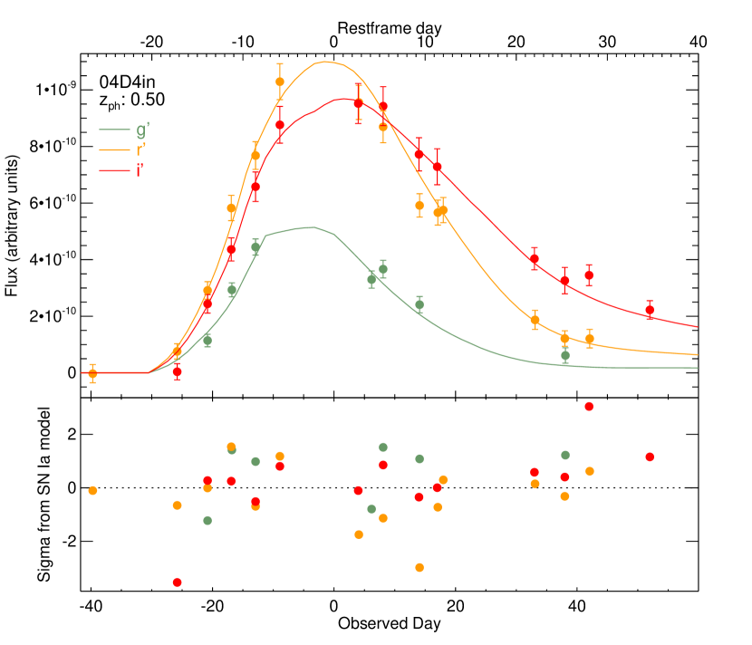
Figure 1.— SN Ia lightcurve fit to real-time data for an example SN candidate that was spectroscopically confirmed as an SN Ia. Data are fit after each photometric point is acquired, solving for the redshift (the SN photo-z). If the fit is consistent with a Ia the candidate is given high priority for spectroscopic follow-up. The predicted redshift from the fit is $z=0.50$, the actual redshift from spectroscopy is 0.516.

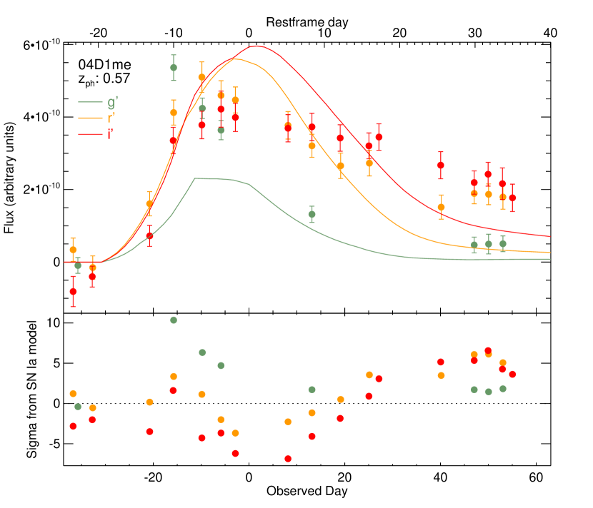
Figure 2.— A SN Ia lightcurve fit to an SN candidate that was eventually spectroscopically identified as a Type II-P. Because the data are not a good fit to an SN Ia lightcurve, such candidates are lowered in priority for spectroscopic follow-up. Even at early times it is apparent that the candidate is not an SN Ia because it is too blue. The formal prediction for the SN photo-z (under the assumption that the candidate is an SN Ia) is 0.56. The spectroscopic redshift is $z=0.256$ — much lower because SNe II are $\sim 1.5$ mag fainter than SNe Ia at a given redshift.

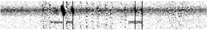
Figure 3.— Section of a two-dimensional nod and shuffle sky-subtracted spectrum. The wavelength solution is applied to the 2D spectrum and the positions of common galaxy lines are overplotted. Wavelength increases to the right; the spatial direction is vertical. The supernova is blended with the host galaxy, but the galaxy emission lines are apparent as the dark diagonal lines. The galaxy lines are slanted due to the rotation of the galaxy. Note the excellent sky subtraction – the subtracted sky lines are the vertical bands of increased poisson noise, but lack systematic residuals.

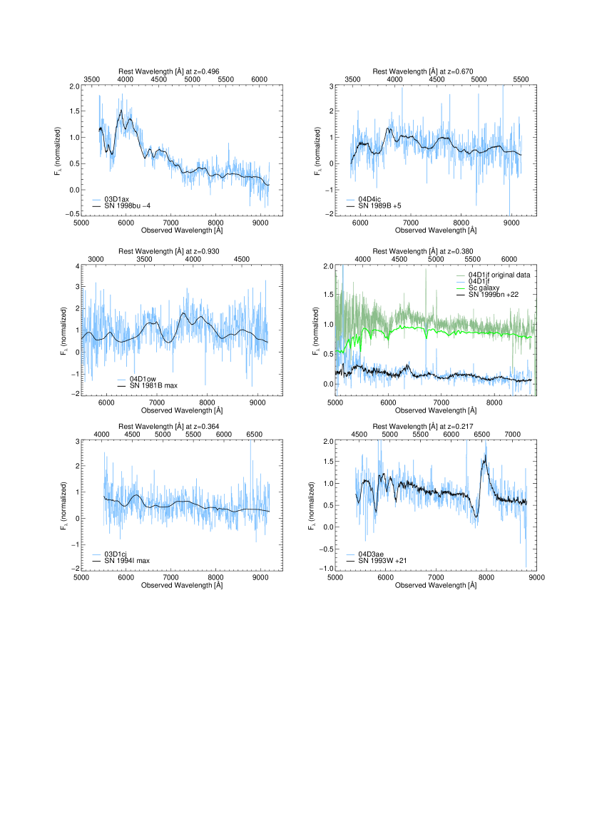
Figure 4.— Spectra of SNLS candidates observed by Gemini. One spectrum from each SN Ia confidence index is shown as an example. All other spectra are available online. When there is only minor galaxy subtraction, only the subtracted spectrum (rebinned to 5Å)is shown. In cases where the galaxy subtraction is important, the original (unbinned) spectrum, the galaxy subtracted spectrum and the smoothed host galaxy that was subtracted are shown. Top-left: 5 (Certain Ia), the Si 4000Å feature is obvious; top-right: 4 (Highly probable Ia), all features match, but at this phase the Si 4000Å feature is not a definitive detection; middle-left: 3 (Probable Ia) an SN Ia is the best fit, but the lower S/N at high redshift leaves some room for doubt; middle-right: 2 (Unidentified), significant host contamination, combined with the fact that many SN types look similar at a late phase means that this SN type is uncertain, despite the match to an SN Ia shown; bottom-left: 1 (Probably not a Ia) An SN Ic is a good fit to the spectrum, but the redshift is uncertain and the S/N is too low to make a definitive classification; bottom-right: 0 (Certainly not a Ia), in this case a Type II. For Index 5, 4, 3, 1, and 0 the gray line (light blue online) shows the data after host galaxy subtraction (if necessary), rebinned to 5Å. For Index 2, the top gray line (dark green) shows the original data, overplotted with the best-fit host galaxy template (bold lighter green). The lower gray line (light blue) shows the data after host subtraction and rebinning — the SN type could not be identified.

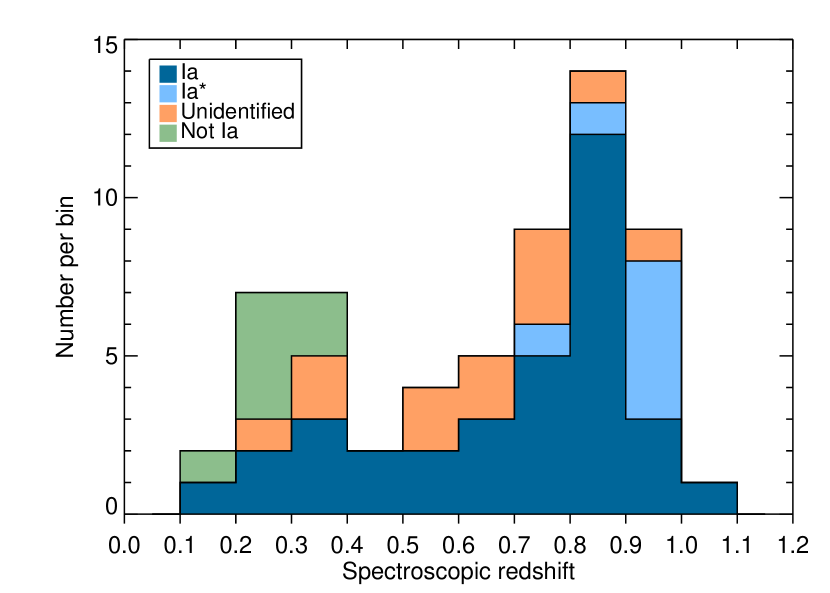
Figure 5.— Histogram of the redshifts of candidates observed by Gemini, where the highest redshift candidates were usually observed. Note that SN Ia classifications are less certain (Ia*) at higher redshifts where the S/N is lower and scarce restframe UV observations must be used to classify the SN. Non-Ia candidates were typically at a lower redshift than that predicted for an SN Ia using the SN photo-z, since core collapse SNe are generally fainter than SNe Ia. The median redshift of SNe Ia/Ia* is 0.81.

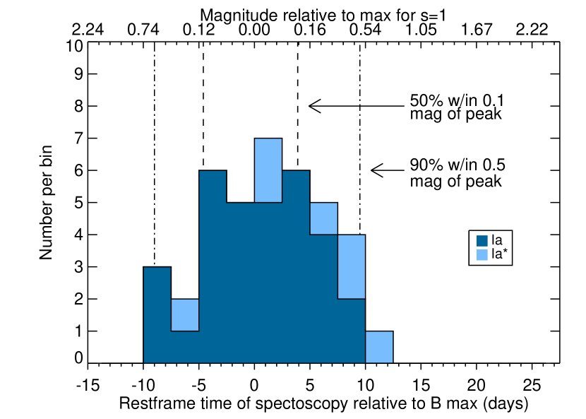
Figure 6.— Histogram of rest frame epoch relative to restframe B-band maximum light for Type Ia/Ia* SNe. Since we can predict the time of maximum light before a candidate is sent for spectroscopy, we can plan the observations so that the contrast between the SN and the host galaxy is at a maximum. More than 50% of SNe were observed within 0.1 mag of maximum light, and 90% of SNe were observed within 0.5 mag of maximum. It is easier to classify SNe Ia with certainty if spectra are taken just before maximum light.

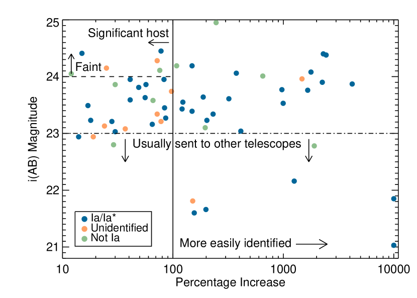
Figure 7.— i′ Magnitude at time of spectroscopy versus percentage increase. Typically candidates were only sent to Gemini if $23<\rm i\arcmin\ <24.5$. When the candidate is brighter than the host (greater than 100% increase) it is identified 93% of the time.

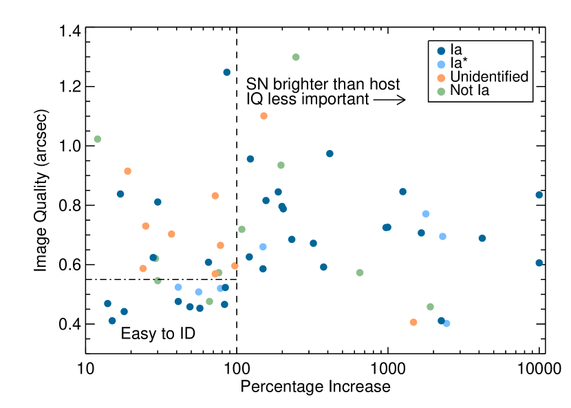
Figure 8.— Image quality (IQ) at the time of spectroscopy versus percentage increase at the time of spectroscopy. If the SN was brighter than the host (% increase $>$ 100), IQ plays a less significant role in determining whether a candidate is identified. However, candidates can still be identified in the presence of significant host contamination if the seeing is exceptional. If the IQ was less than 0.55$\arcsec$ candidates were identified 88% of the time (only SNe with both a percentage increase and IQ measurement are plotted in the figure).

Figure 9.— Rest frame epoch of spectroscopy relative to rest B-band maximum light as determined by fits to the lightcurve and fits to the spectra. The line shows where SNe should lie if the lightcurve epoch is equal to the spectroscopic epoch – it is not a fit to the data. The lightcurve epoch is from fits to the final reductions of the lightcurve data where possible, but in some cases it is from fits to preliminary (real-time) data. The open circle is a spectroscopically peculiar (SN 2001ay-like) SN for which there are few templates in the spectroscopic matching library. The inset shows the difference between the spectroscopic epoch and the lightcurve epoch as a function of lightcurve epoch, with the same units as the larger graph. Note that from -4d to +4d, SN Ia spectra are similar, so an automatic determination of a date from fits to the spectrum can be difficult. There is also a tendency to overpredict the spectroscopic phase at early times. This is probably due to the scarcity of early SN Ia spectra.

Table 1SNLS SN Candidates Observed with Gemini

SN	RA (2000)	Dec (2000)	UT Date	Exp.	Mode	$\lambda_{\rm c}$	IQ	Mag	%I
03D1as	02:24:24.520	-04:21:40.19	2003-09-27	6000	N+S	720	0.41	23.96	1475
03D1ax	02:24:23.320	-04:43:14.41	2003-09-29	2400	C	720	0.61	23.16	65
03D1bk	02:26:27.410	-04:32:11.99	2003-09-28	4800	N+S	720	0.47	23.95	83
03D1cj	02:26:25.081	-04:12:39.89	2003-10-26	5400	N+S	720	0.57	24.11	76
03D1cm	02:24:55.288	-04:23:03.68	2003-10-27	5400	N+S	720	0.72	23.77	970
03D1co	02:26:16.238	-04:56:05.76	2003-11-01	7200	N+S	720	0.84	23.64	188
03D1ew	02:24:14.088	-04:39:56.98	2003-12-21	7200	N+S	720	0.71	23.76	1661
03D1fp	02:26:03.073	-04:08:02.02	2003-12-26	7200	N+S	720	0.55	23.86	30
03D1fq	02:26:55.683	-04:18:08.10	2003-12-24	5400	N+S	720	0.48	23.59	41
03D4cj	22:16:06.660	-17:42:16.72	2003-08-26	2700	C	680	0.83	21.85	10000
03D4ck	22:15:08.910	-17:56:02.17	2003-08-27	2400	C	680	0.46	22.78	1905
03D4cn	22:16:34.600	-17:16:13.55	2003-08-27	4800	C	720	0.46	23.81	49
03D4cy	22:13:40.460	-17:40:53.90	2003-09-26	5400	N+S	720	0.59	24.19	149
03D4cz	22:16:41.870	-17:55:34.54	2003-09-27	3600	C	720	0.41	24.41	15
03D4fd	22:16:14.471	-17:23:44.37	2003-10-24	3600	N+S	720	0.67	23.61	321
03D4fe	22:16:08.844	-17:55:19.21	2003-10-24	3600	N+S	720	0.48	23.58	66
03D4gl	22:14:44.177	-17:31:44.47	2003-10-29	3600	N+S	720	0.63	23.43	121
04D1de	02:26:35.925	-04:25:21.65	2004-08-17	7200	N+S	720	0.51	23.63	56
04D1dr	02:27:23.905	-04:51:27.43	2004-08-14	5400	N+S	720	0.57	24.28	72
04D1hd	02:26:08.850	-04:06:35.22	2004-09-13	2400	C	680	0.85	22.16	1254
04D1ho	02:24:44.856	-04:39:15.55	2004-09-16	3600	C	720	0.59	23.13	24
04D1hy	02:24:08.678	-04:49:52.22	2004-09-11	5400	N+S	720	0.73	23.53	996
04D1jf	02:25:18.914	-04:49:09.05	2004-10-13	2400	C	680	0.92	22.94	19
04D1ln	02:25:53.482	-04:27:03.75	2004-10-17	2400	C	680	0.62	22.80	29
04D1ow	02:26:42.708	-04:18:22.55	2004-11-08	5400	N+S	720	0.69	23.87	4201
04D2aa	10:02:02.100	+02:40:51.76	2004-01-23	7320	N+S	720	0.58	24.19	$\cdots$
04D2ad	10:00:08.093	+02:39:01.40	2004-01-22	7320	N+S	720	0.54	24.17	$\cdots$
04D2ae	10:01:52.414	+02:13:21.11	2004-01-21	5490	N+S	720	0.75	23.64	$\cdots$
04D3aa	14:16:49.935	+52:45:31.12	2004-01-30	5400	N+S	720	1.02	24.05	12
04D3ae	14:22:21.569	+52:21:39.21	2004-01-25	2400	C	680	0.94	23.10	196
04D3ax	14:22:39.072	+52:51:52.57	2004-01-28	5400	N+S	720	1.30	24.95	246
04D3bf	14:17:45.096	+52:28:04.31	2004-02-17	2700	C	680	$\cdots$	23.16	$\cdots$
04D3dd	14:17:48.431	+52:28:14.72	2004-04-25	5400	N+S	720	0.59	24.06	375
04D3de	14:22:13.503	+52:17:09.71	2004-04-27	7200	N+S	720	0.57	24.01	651
04D3fj	14:19:50.703	+52:41:31.84	2004-04-28	7200	N+S	720	0.72	24.19	108
04D3fq	14:16:57.906	+52:22:46.53	2004-04-26	5400	N+S	720	0.97	23.04	412
04D3gu	14:22:07.359	+52:38:54.60	2004-05-22	4800	C	720	1.03	22.60	6
04D3gx	14:20:13.678	+52:16:58.60	2004-05-21	7200	N+S	720	0.40	24.38	2439
04D3hn	14:22:06.878	+52:13:43.46	2004-05-22	4800	C	720	0.47	22.94	14
04D3kr	14:16:35.937	+52:28:44.20	2004-06-16	2400	C	680	0.82	21.60	156
04D3lp	14:19:50.927	+52:30:11.85	2004-05-27	5400	N+S	720	0.52	24.45	78
04D3lu	14:21:08.009	+52:58:29.74	2004-06-23	3600	N+S	720	0.84	23.49	17
04D3mk	14:19:25.830	+53:09:49.56	2004-06-19	4320	N+S	720	1.25	23.27	86
04D3ml	14:16:39.107	+53:05:35.66	2004-06-20	3600	N+S	720	0.41	23.90	2252
04D3nc	14:16:18.224	+52:16:26.09	2004-07-13	2400	C	720	0.66	23.39	149
04D3nh	14:22:26.729	+52:20:00.92	2004-06-23	1800	C	680	0.80	21.66	199
04D3nq	14:20:19.193	+53:09:15.90	2004-07-14	1500	C	680	0.61	21.03	10000
04D3nr	14:22:38.526	+52:38:55.89	2004-07-15	7200	N+S	720	0.69	24.40	2300
04D3ny	14:18:56.332	+52:11:15.06	2004-07-10	5400	N+S	720	0.79	23.23	203
04D3oe	14:19:39.381	+52:33:14.21	2004-07-11	3600	N+S	720	0.62	23.21	28
04D3og	14:20:39.748	+53:01:15.02	2004-07-19	2700	C	720	1.10	21.81	151
04D3pd	14:22:33.506	+52:13:47.77	2004-07-18	3600	N+S	720	0.83	23.34	72
04D4dm	22:15:25.470	-17:14:42.71	2004-07-18	3600	N+S	720	0.96	23.55	123
04D4ec	22:16:29.286	-18:11:04.13	2004-07-19	3600	N+S	720	0.70	23.08	37
04D4ft	22:14:31.097	-17:40:19.74	2004-08-12	3600	C	720	0.67	23.21	78
04D4gg	22:16:09.268	-17:17:39.98	2004-08-16	3600	C	720	0.81	23.03	30
04D4hu	22:15:36.193	-17:50:19.81	2004-09-18	5400	N+S	720	0.52	23.45	84
04D4hx	22:13:40.587	-17:23:03.35	2004-09-16	5400	N+S	720	0.73	24.15	25
04D4ic	22:14:21.841	-17:56:36.43	2004-09-12	5160	N+S	720	0.69	23.34	231
04D4ih	22:17:17.041	-17:40:38.74	2004-10-07	5400	N+S	720	0.52	23.95	41
04D4ii	22:15:55.645	-17:39:27.09	2004-09-15	7200	N+S	720	0.45	23.86	57
04D4im	22:15:00.885	-17:23:45.84	2004-10-10	7200	N+S	720	0.44	23.23	18
04D4jy	22:13:51.605	-17:24:18.13	2004-10-14	8881	N+S	720	0.77	24.08	1779
04D4kn	22:15:04.324	-17:19:45.05	2004-10-19	5400	N+S	720	0.60	23.74	97

Note. — SNe observed using Gemini GMOS during semesters 2003B, 2004A, and 2004B. Observations from Gemini-N except where noted. Observational setup: R400 Grating, 0.75″slit, binning $2\times 2$. One observation is not listed in this table, SNLS 04D3bf, because it was observed at Gemini-S after the SN had faded to get the host redshift.

Table 2Derived properties for SNLS SN Candidates Observed with Gemini.

SN	z	$\pm$	Type	CI	$\tau_{\rm LC}$	$\pm$	$\tau_{\rm spec}$	z from
03D1as	0.872	0.001	SN:	2	$\cdots$	$\cdots$	$\cdots$	O II:
03D1ax	0.496	0.001	SN Ia	5	-3.0	0.1	-3.3	H&K
03D1bk	0.8650	0.0005	SN Ia	5	-6.3	0.1	-2.1	H&K, H$\beta$, H$\gamma$
03D1cj	0.364	0.001	SN Ib/c:	1	$\cdots$	$\cdots$	$\cdots$	H$\alpha$, O III
03D1cm	0.87	0.02	SN Ia	4	-5.0	0.3	2.4	SN
03D1co	0.68	0.01	SN Ia	5	-4.8	0.3	-1.2	SN
03D1ew	0.868	0.001	SN Ia	5	0.9	0.4	-0.2	O II
03D1fp	0.270	0.001	SN IIb	0	$\cdots$	$\cdots$	$\cdots$	H$\alpha$, H$\beta$, N II, O II, S II
03D1fq	0.80	0.02	SN Ia	4	-1.6	0.3	2.2	SN
03D4cj	0.27	0.01	SN Ia	5	-9.7	0.1	-6.9	SN
03D4ck	0.189	0.001	SN IIn	0	$\cdots$	$\cdots$	$\cdots$	SN
03D4cn	0.818	0.001	SN Ia	4	-0.5	0.6	2.8	O II, O III, H$\beta$
03D4cy	0.9271	0.0005	SN Ia	4	5.3	0.3	7.7	O II
03D4cz	0.695	0.001	SN Ia	4	9.4	0.1	8.7	H&K, G-band
03D4fd	0.791	0.003	SN Ia	5	-1.6	0.3	-1.5	O II
03D4fe	?	$\cdots$	SN:	1	$\cdots$	$\cdots$	$\cdots$	$\cdots$
03D4gl	0.56	0.01	SN Ia	4	-9.0	0.2	-6.0	SN
04D1de	0.7677	0.0002	SN Ia*	3	-6.8	0.1	-4.5	O II, O III, H$\beta$, poss H&K
04D1dr	0.6414	0.0003	SN:	2	$\cdots$	$\cdots$	$\cdots$	O II, O III, H$\beta$, H$\gamma$
04D1hd	0.3685	0.0005	SN Ia	5	-4.8	0.1	-4.0	O III, weak O II
04D1ho	0.7012	0.0004	SN	2	$\cdots$	$\cdots$	$\cdots$	O II, O III, H&K, H$\beta$, H$\gamma$
04D1hy	0.85	0.02	SN Ia	5	-3.5	0.3	-3.2	SN
04D1jf	0.3800	0.0002	SN:	2	$\cdots$	$\cdots$	$\cdots$	O II, O III, H$\beta$
04D1ln	0.2072	0.0002	SN II-P	0	$\cdots$	$\cdots$	$\cdots$	H$\alpha$, N II, S II
04D1ow	0.93	0.02	SN Ia	4	2.6	0.2	-0.8	SN
04D2aa	?	$\cdots$	SN:	2	$\cdots$	$\cdots$	$\cdots$	$\cdots$
04D2ad	0.6802	0.0002	SN:	2	$\cdots$	$\cdots$	$\cdots$	O II, O III, H$\beta$
04D2ae	0.843	0.001	SN Ia	4	0.0	0.1	-1.5	H&K
04D3aa	0.2045	0.0002	SN II	0	$\cdots$	$\cdots$	$\cdots$	H$\alpha$, H$\beta$, O III, S II
04D3ae	0.217	0.001	SN II	0	$\cdots$	$\cdots$	$\cdots$	H$\alpha$, O III
04D3ax	0.3558	0.0002	SN II:	1	$\cdots$	$\cdots$	$\cdots$	H$\alpha$, H$\beta$, O III
04D3bf	0.1560	0.0005	SN Ia	5	$\cdots$	$\cdots$	15.1	O II, O III, S II, H$\alpha$, H$\beta$
04D3dd	1.01	0.02	SN Ia	4	2.9	0.3	-1.4	SN
04D3de	?	$\cdots$	SN II-P	0	$\cdots$	$\cdots$	$\cdots$	$\cdots$
04D3fj	?	$\cdots$	SN:	1	$\cdots$	$\cdots$	$\cdots$	$\cdots$
04D3fq	0.73	0.01	SN Ia	4	0.8	0.3	3.6	SN
04D3gu	0.748	0.001	SN:	2	$\cdots$	$\cdots$	$\cdots$	H&K, Balmer, weak O II
04D3gx	0.91	0.02	SN Ia*	3	10.8	0.2	8.3	SN
04D3hn	0.5516	0.0003	SN Ia	5	7.2	0.1	4.9	H&K, Balmer
04D3kr	0.3373	0.0002	SN Ia	5	4.4	0.1	1.7	O II, O III, H$\beta$
04D3lp	0.983	0.001	SN Ia*	3	1.0	0.2	-1.2	O II
04D3lu	0.8218	0.0002	SN Ia	4	5.5	0.1	5.6	H&K
04D3mk	0.813	0.001	SN Ia	5	-2.4	0.1	1.2	O II, H&K
04D3ml	0.95	0.02	SN Ia	4	-1.8	0.3	1.1	SN
04D3nc	0.817	0.001	SN Ia*	3	7.2	0.2	$\cdots$	poss O II
04D3nh	0.3402	0.0002	SN Ia	5	3.5	0.1	3.7	H$\alpha$, H$\beta$, O II, poss H&K
04D3nq	0.22	0.01	SN Ia	5	8.1	0.1	8.8	SN
04D3nr	0.96	0.02	SN Ia*	3	8.1	0.3	3.9	SN
04D3ny	0.81	0.02	SN Ia	5	1.6	0.2	2.5	SN
04D3oe	0.756	0.001	SN Ia	4	1.4	0.1	1.8	H&K
04D3og	0.352	0.001	SN	2	$\cdots$	$\cdots$	$\cdots$	H$\alpha$, H$\beta$, O II, N II, S II
04D3pd	0.760	0.001	SN:	2	$\cdots$	$\cdots$	$\cdots$	H$\beta$, O II, O III
04D4dm	0.811	0.001	SN Ia	4	2.7	0.2	-0.7	O II, O III
04D4ec	0.593	0.001	SN:	2	$\cdots$	$\cdots$	$\cdots$	O II, O III, H$\beta$, H$\gamma$
04D4ft	0.2666	0.0002	SN	2	$\cdots$	$\cdots$	$\cdots$	O III, H$\alpha$, H$\beta$
04D4gg	0.4238	0.0004	SN Ia	5	-9.7	0.1	-10.0	O II, O III, H$\alpha$, H$\beta$, H$\gamma$
04D4hu	0.7027	0.0003	SN Ia	5	5.2	0.5	5.0	O II, O III, H$\beta$
04D4hx	0.545	0.005	SN:	2	$\cdots$	$\cdots$	$\cdots$	4000Å break, poss H&K
04D4ic	0.68	0.02	SN Ia	4	2.5	0.3	4.8	SN
04D4ih	0.934	0.001	SN Ia*	3	8.7	0.2	5.6	O II, H&K, some Balmer
04D4ii	0.866	0.001	SN Ia	5	-4.6	0.2	-3.5	O II
04D4im	0.7510	0.0005	SN Ia	4	0.7	0.2	0.2	H&K, H$\delta$
04D4jy	0.93	0.02	SN Ia*	3	2.0	0.4	0.0	SN
04D4kn	0.9095	0.0005	SN:	2	$\cdots$	$\cdots$	$\cdots$	O II, H&K, Balmer

Note. — Derived properties for SNe listed in Table 1. A colon denotes uncertainty.

Table 3Ia Confidence Index and Host Type.

CI	Abs.	Emis.	None
5	2	11	5
4	5	3	8
3	0	4	3
2	1	11	1
1	0	2	2
0	0	4	2

Note. — Note that probable and certain core collapse SNe (index 0 and 1) do not occur in absorption line galaxies.

References

- Blondin et al. (2005) Blondin, S., Walsh, J. R., Leibundgut, B., & Sainton, G. 2005, A&A, 431, 757
- Cardelli et al. (1989) Cardelli, J. A., Clayton, G. C., & Mathis, J. S. 1989, ApJ, 345, 245
- Coil et al. (2000) Coil, A. L., Matheson, T., Filippenko, A. V., Leonard, D. C., Tonry, J., Riess, A. G., Challis, P., Clocchiatti, A., Garnavich, P. M., Hogan, C. J., Jha, S., Kirshner, R. P., Leibundgut, B., Phillips, M. M., Schmidt, B. P., Schommer, R. A., Smith, R. C., Soderberg, A. M., Spyromilio, J., Stubbs, C., Suntzeff, N. B., & Woudt, P. 2000, ApJ, 544, L111
- Filippenko (1997) Filippenko, A. V. 1997, ARA&A, 35, 309
- Fioc & Rocca-Volmerange (1997) Fioc, M., & Rocca-Volmerange, B. 1997, A&A, 326, 950
- Glazebrook & Bland-Hawthorn (2001) Glazebrook, K., & Bland-Hawthorn, J. 2001, PASP, 113, 197
- Hook et al. (2005) Hook, I., et al. 2005, AJ, submitted
- Hook et al. (2004) Hook, I. M., Jørgensen, I., Allington-Smith, J. R., Davies, R. L., Metcalfe, N., Murowinski, R. G., & Crampton, D. 2004, PASP, 116, 425
- Howell & Wang (2002) Howell, D. A., & Wang, L. 2002, Bulletin of the American Astronomical Society, 34, 1256
- Kinney et al. (1996) Kinney, A. L., Calzetti, D., Bohlin, R. C., McQuade, K., Storchi-Bergmann, T., & Schmitt, H. R. 1996, ApJ, 467, 38
- Krisciunas et al. (1987) Krisciunas, K., Sinton, W., Tholen, K., Tokunaga, A., Golisch, W., Griep, D., Kaminski, C., Impey, C., & Christian, C. 1987, PASP, 99, 887+
- Li et al. (2001) Li, W., Filippenko, A. V., Treffers, R. R., Riess, A. G., Hu, J., & Qiu, Y. 2001, ApJ, 546, 734
- Lidman et al. (2005) Lidman, C., Howell, D. A., Folatelli, G., Garavini, G., Nobili, S., Aldering, G., Amanullah, R., Antilogus, P., Astier, P., Blanc, G., Burns, M. S., Conley, A., Deustua, S. E., Doi, M., Ellis, R., Fabbro, S., Fadeyev, V., Gibbons, R., Goldhaber, G., Goobar, A., Groom, D. E., Hook, I., Kashikawa, N., Kim, A. G., Knop, R. A., Lee, B. C., Mendez, J., Morokuma, T., Motohara, K., Nugent, P. E., Pain, R., Perlmutter, S., Prasad, V., Quimby, R., Raux, J., Regnault, N., Ruiz-Lapuente, P., Sainton, G., Schaefer, B. E., Schahmaneche, K., Smith, E., Spadafora, A. L., Stanishev, V., Walton, N. A., Wang, L., Wood-Vasey, W. M., & Yasuda (The Supernova Cosmology Project), N. 2005, A&A, 430, 843
- Matheson et al. (2005) Matheson, T., Blondin, S., Foley, R. J., Chornock, R., Filippenko, A. V., Leibundgut, B., Smith, R. C., Sollerman, J., Spyromilio, J., Kirshner, R. P., Clocchiatti, A., Aguilera, C., Barris, B., Becker, A. C., Challis, P., Covarrubias, R., Garnavich, P., Hicken, M., Jha, S., Krisciunas, K., Li, W., Miceli, A., Miknaitis, G., Prieto, J. L., Rest, A., Riess, A. G., Salvo, M. E., Schmidt, B. P., Stubbs, C. W., Suntzeff, N. B., & Tonry, J. L. 2005, AJ, 129, 2352
- Perlmutter et al. (1999) Perlmutter, S., Aldering, G., Goldhaber, G., Knop, R. A., Nugent, P., Castro, P. G., Deustua, S., Fabbro, S., Goobar, A., Groom, D. E., Hook, I. M., Kim, A. G., Kim, M. Y., Lee, J. C., Nunes, N. J., Pain, R., Pennypacker, C. R., Quimby, R., Lidman, C., Ellis, R. S., Irwin, M., McMahon, R. G., Ruiz-Lapuente, P., Walton, N., Schaefer, B., Boyle, B. J., Filippenko, A. V., Matheson, T., Fruchter, A. S., Panagia, N., Newberg, H. J. M., Couch, W. J., & The Supernova Cosmology Project. 1999, ApJ, 517, 565
- Perlmutter et al. (1995) Perlmutter, S., Pennypacker, C. R., Goldhaber, G., Goobar, A., Muller, R. A., Newberg, H. J. M., Desai, J., Kim, A. G., Kim, M. Y., Small, I. A., Boyle, B. J., Crawford, C. S., McMahon, R. G., Bunclark, P. S., Carter, D., Irwin, M. J., Terlevich, R. J., Ellis, R. S., Glazebrook, K., Couch, W. J., Mould, J. R., Small, T. A., & Abraham, R. G. 1995, ApJ, 440, L41
- Pritchet et al. (2004) Pritchet, C. J., et al. 2004, ArXiv Astrophysics e-prints
- Riess et al. (1998) Riess, A. G., Filippenko, A. V., Challis, P., Clocchiatti, A., Diercks, A., Garnavich, P. M., Gilliland, R. L., Hogan, C. J., Jha, S., Kirshner, R. P., Leibundgut, B., Phillips, M. M., Reiss, D., Schmidt, B. P., Schommer, R. A., Smith, R. C., Spyromilio, J., Stubbs, C., Suntzeff, N. B., & Tonry, J. 1998, AJ, 116, 1009
- Riess et al. (1997) Riess, A. G., Filippenko, A. V., Leonard, D. C., Schmidt, B. P., Suntzeff, N., Phillips, M. M., Schommer, R., Clocchiatti, A., Kirshner, R. P., Garnavich, P., Challis, P., Leibundgut, B., Spyromilio, J., & Smith, R. C. 1997, AJ, 114, 722
- Riess et al. (2004) Riess, A. G., Strolger, L., Tonry, J., Tsvetanov, Z., Casertano, S., Ferguson, H. C., Mobasher, B., Challis, P., Panagia, N., Filippenko, A. V., Li, W., Chornock, R., Kirshner, R. P., Leibundgut, B., Dickinson, M., Koekemoer, A., Grogin, N. A., & Giavalisco, M. 2004, ApJ, 600, L163
- Schlegel et al. (1998) Schlegel, D. J., Finkbeiner, D. P., & Davis, M. 1998, ApJ, 500, 525
- Sullivan et al. (2004) Sullivan, M., et al. 2004, ArXiv Astrophysics e-prints
- Sullivan et al. (2005) —. 2005, AJ, submitted
- van Dokkum (2001) van Dokkum, P. G. 2001, PASP, 113, 1420