Fitting Formula for Flux Scintillation of Compact Radio Sources

Abstract

We present a fitting function to describe the statistics of flux modulations caused by interstellar scintillation. The function models a very general quantity: the cross-correlation of the flux observed from a compact radio source of finite angular size observed at two frequencies and at two positions or times. The formula will be useful for fitting data from sources such as intra-day variables and gamma-ray burst afterglows. These sources are often observed at relatively high frequencies (several gigahertz) where interstellar scattering is neither very strong nor very weak, so that asymptotic formulae are inapplicable.

1 Introduction

Ever since its initial discovery in the signals received from radio pulsars, interstellar scattering and scintillation has proved to be a useful tool in radio astronomy (see Rickett 1990, 2001; Narayan 1993; Hewish 1993 for reviews). It provides unique information on small-scale turbulent fluctuations in the ionized interstellar medium (e.g., Armstrong, Cordes & Rickett 1981; Wilkinson, Narayan & Spencer 1994) and on the sizes of compact radio sources. The latter application has contributed to progress in several areas of astrophysics: radio pulsars (e.g., Roberts & Ables 1982; Cordes, Weisberg & Boriakoff 1983; Wolszczan & Cordes 1987; Gwinn et al. 1997), intra-day variables (e.g., Rickett et al. 1995, 2001; Lovell et al. 2003) and gamma-ray burst afterglows (e.g., Goodman 1997; Frail et al. 1997; Taylor et al. 1997).

The fundamental quantity in scintillation theory is the correlation of flux variations of a distant source observed at two positions separated by transverse distance $r$ on the observer plane. Since each flux is the square of the local electric field, the quantity of interest is a fourth order correlation of the electric field (see eq. 2). To interpret scintillation data, we need to calculate the expectation value of this fourth moment as a function of the strength of the turbulent fluctuations in the scattering medium, the shape and size of the radio source, the observing frequency, etc.

The scattering of radio waves in the interstellar medium may be characterized by two dimensionless parameters (eq. 6): $U$ which measures the strength of the scattering, and $\alpha$ which describes the power spectrum of the fluctuations. The turbulence in the interstellar medium appears to be well-described by a Kolmogorov scaling, which corresponds to $\alpha=5/3$. Hence, the scattering medium along any line of sight is determined by just $U$; however, $U$ varies from one direction to another, and also with frequency in a given direction (see eq. 19). Analytical results are available for the flux correlation function in the limit of both very weak scattering ($U\ll 1$) and very strong scattering ($U\gg 1$) (e.g., Goodman & Narayan, 1995; Rickett 1990; and references therein). In the latter regime, the scintillation is known to occur on two very different scales, determined by diffractive and refractive effects.

While a great deal of interesting work on interstellar scintillation has been done using asymptotic results, many observations correspond to the difficult intermediate regime where $U$ is neither $\ll 1$ nor $\gg 1$; no analytical results are available in this transition regime. For typical high lines of sight through the interstellar medium at high Galactic latitudes, the transition regime occurs at radio frequencies $\sim 5-10$ GHz, a frequency of much interest for both intra-day variables and gamma-ray burst afterglows (but less so for pulsars which, because of their steep radio spectra, are usually observed at lower frequencies where asymptotic strong scattering results apply). Some very approximate formulae have been proposed for the transition regime (e.g., Walker 1998). However, for accurate results, one has to resort to numerical computations of the scintillation correlation function, which is technically challenging and has been rarely attempted.

We describe in this paper numerical computations of the scintillation correlation function for a wide range of values of the scattering parameter $U$, spatial separation $r$, source size $r_{s}$ (defined in eqs. 15–18) and frequency difference $\eta$ (defined in eq. 5). Using the numerical results we have developed a fitting function for the flux correlation that is valid for all values of $U$. The function asymptotes to the appropriate analytical results in the limits $U\ll 1$ (very weak scattering) and $U\gg 1$ (very strong scattering) and agrees well with numerical results in the transition regime in between.

In §2 we introduce the basic fourth order moment of interest to flux scintillation observations, and in §3 we explain how we numerically compute this quantity. In §4 we present our fitting formula, which agrees well with the numerical results. We conclude in §5 with a brief summary. We present in Appendices A-C technical details, including some asymptotic results useful as checks of our fitting functions, and a discussion of parabolic arcs in secondary spectra.

2 Thin-screen theory

In the thin-screen approximation, one imagines that the turbulence affecting radio-wave propagation is concentrated in a narrow layer perpendicular to the line of sight. This is sometimes not far from the truth, although it would usually be more accurate to assume a number of scattering screens; but the opposite limit of homogeneously distributed turbulence is probably the exception rather than the rule. The observer lies in a parallel plane at distance $z_{\rm screen}$ from the screen, and the source is behind the screen at distance $z_{\rm source}$ from it. Waves propagate freely from the source to the screen, where they suffer a phase shift $\phi({\bf x})$ that depends upon the two-dimensional position ${\bf x}$ within the screen, and thence travel freely again to the observer’s plane. The distortion of the phase fronts at the screen leads to modulations of the flux on the observer’s plane, through a combination of refractive focusing and diffractive interference. It is useful to define an effective distance

$$z\equiv\rm\left(\frac{1}{z_{\rm screen}}+\frac{1}{z_{\rm source}}\right)^{-1}$$ (1)

from observer to screen. This allows us to analyze the problem as if the source were infinitely distant and the wavefronts were planar before encountering the screen.

We follow the notation of Goodman & Narayan (1989, henceforth GN89), who discuss the mutual coherence function

$$\Gamma_{4}({\bf b};{\bf r};\nu_{1},\nu_{2})\equiv\left\langle E\left(\frac{1}{2}{\bf b},\nu_{1}\right)E^{*}\left(-\frac{1}{2}{\bf b},\nu_{1}\right)E\left({\bf r}+\frac{1}{2}{\bf b},\nu_{2}\right)E^{*}\left({\bf r}-\frac{1}{2}{\bf b},\nu_{2}\right)\right\rangle\,,$$ (2)

where $E({\bf r},\nu)$ is the electric field due to a source of unit strength measured at vector position ${\bf r}$ on the observer’s plane (a plane perpendicular to the line of sight to the source) at radio frequency $\nu$. As written above, $\Gamma_{4}$ is useful for studying the correlation between measurements of visibility made with two two-element interferometers having the same baseline ${\bf b}$ but phase centers separated by ${\bf r}$, and operating at different frequencies $\nu_{1}$ and $\nu_{2}$. In this paper, we are interested in flux correlations rather than visibilities, so we set ${\bf b}\to 0$. Positions ${\bf 0}$ and ${\bf r}$ then represent two positions at which the flux is measured. The measurements may be done by two telescopes simultaneously, or by the same telescope at different times. In the latter case, the interstellar turbulence responsible for phase changes in $E$ is assumed “frozen” on timescales of interest, so that ${\bf r}={\bf v}_{\perp}t$, where ${\bf v}_{\perp}$ is the effective transverse velocity of the line of sight through the interstellar medium. The angle brackets denote an ensemble average over realizations of the turbulence.

Appendix A derives formula (A4) for the flux correlation $\Gamma_{4}({\bf 0};{\bf r};\nu_{1},\nu_{2})$ in terms of the phase structure function

$$D(\Delta{\bf x})\equiv\left\langle\left[\phi(\Delta{\bf x},\lambda)-\phi({\bf 0},\lambda)\right]^{2}\right\rangle$$

evaluated at the geometric mean wavelength

$$\lambda\equiv\sqrt{\lambda_{1}\lambda_{2}}$$ (3)

of the two observing wavelengths $\lambda_{1,2}\equiv c/\nu_{1,2}$, and in terms of a Fresnel scale defined with the arithmetic mean,

$$r_{\rm F}\equiv\left[\frac{(\lambda_{1}+\lambda_{2})z}{4\pi}\right]^{1/2}\,,$$ (4)

and a dimensionless frequency difference

$$\eta\equiv\frac{\lambda_{2}-\lambda_{1}}{\lambda_{1}+\lambda_{2}}~{}:~{}~{}0\leq|\eta|<1\,.$$ (5)

In this paper, we restrict our attention to power-law structure functions

$$D(\Delta{\bf x})=U\left(\frac{\Delta{\bf x}}{r_{\rm F}}\right)^{\alpha}\,,$$ (6)

and unless otherwise specified, we assume $\alpha=5/3$ (the “Kolmogorov” value). Thus $U$ is a dimensionless number describing the strength of scattering; it depends upon the observing wavelength (see eq. 19) as well as the intrinsic amplitude of the turbulent electron-density power spectrum, since $D\propto\lambda^{2}$ as a consequence of the plasma dispersion relation. Henceforth we choose units of length such that $r_{\rm F}\equiv 1$. Also, we normalize the mean flux to unity at all frequencies, $\langle F({\bf r},\nu)\rangle=\langle|E({\bf r},\nu)|^{2}\rangle=1$. Writing $W$ rather than $\Gamma_{4}$ for the flux correlation, we have

$$W({\bf r},\eta) \equiv \Gamma_{4}({\bf 0};{\bf r};\nu_{1},\nu_{2})\equiv\left\langle\left|E({\bf 0},\nu_{1})\right|^{2}\left|E({\bf r},\nu_{1})\right|^{2}\right\rangle=\int\frac{d{\bf q}}{(2\pi)^{2}}\,\exp(i{\bf r}\cdot{\bf q})\widetilde{W}({\bf q},\eta),$$ (7)

$$\widetilde{W}({\bf q},\eta) = \exp\left[-\frac{1}{2}F({\bf q},\eta)\right]\int d{\bf s}\,\exp(i{\bf q}\cdot{\bf s})\exp\left[-\frac{1}{2}G({\bf s},{\bf q},\eta)\right],$$ (8)

$$F({\bf q},\eta) \equiv U\left[\frac{(1-\eta)^{\alpha+2}+(1+\eta)^{\alpha+2}}{1-\eta^{2}}\right]\left|{\bf q}\right|^{\alpha},$$ (9)

$$G({\bf s},{\bf q},\eta) \equiv U\left[\left|{\bf s}-\eta{\bf q}\right|^{\alpha}+\left|{\bf s}+\eta{\bf q}\right|^{\alpha}-\left|{\bf s}-{\bf q}\right|^{\alpha}-\left|{\bf s}+{\bf q}\right|^{\alpha}\right]\,.$$ (10)

The quantity $\widetilde{W}({\bf q},\eta)$ will be referred to as the “cross spectrum.” For $\eta=0$ it reduces to the two-dimensional spatial power spectrum of the flux, $\widetilde{W}({\bf q})$.

We know no closed-form results for the integral (8) except at uninteresting values of $\alpha$, so it is necessary to evaluate the integral numerically in general. However, approximate analytic expressions can be obtained in the limits $U\ll 1$ (weak scattering) and $U\gg 1$ (strong scattering), and these are given in Appendix B. They are useful to check the accuracy of the numerical evaluation of the integral (7), and also to guide the choice of functional form for the fitting functions presented in §4.

3 Numerical methods

The integral (8) for the flux cross spectrum $\widetilde{W}({\bf q},\eta)$ proved to be challenging to estimate accurately over the full ranges of $U$, $q$, and $\eta$ required. It is two-dimensional and extends to infinity. Worse, it is only conditionally convergent since $G({\bf s},{\bf q},\eta)\to 0$ as $s/q\to\infty$. And the regions of the ${\bf s}$ plane that dominate the integral vary with the scattering regime.

We experimented with several approaches before settling on the following. The independent variable ${\bf s}$ is resolved into its components parallel and perpendicular to ${\bf q}$: $s_{\parallel}$ & $s_{\perp}$. The inner integration is taken over $s_{\parallel}$ and is calculated by a version of steepest descent in the complex plane $s_{\parallel}\equiv z\equiv x+iy$. That is, at each value of $s_{\perp}$ required by the quadrature scheme for the outer integral, our code estimates

$$\int\limits_{C}\exp\left[iqz~{}+~{}G(z,s_{\perp},q,\eta)\right]\,dz,$$ (11)

where $C$ is a contour which in the first instance is the real axis [$y\equiv 0$, $x\in(-\infty,\infty)$] but which is moved into the upper half plane, where the first exponential in (11) vanishes as $y\to\infty$ since $q\equiv|{\bf q}|>0$. The contour must not, however, be dragged across any of the singularities of

$$G(z,s_{\perp},q,\eta) = U\left\{\left[(z-\eta q)^{2}+s_{\perp}^{2}\right]^{\alpha/2}+\left[(z+\eta q)^{2}+s_{\perp}^{2}\right]^{\alpha/2}\right.$$ (12)

$$\left.-\left[(z-q)^{2}+s_{\perp}^{2}\right]^{\alpha/2}+\left[(z+q)^{2}+s_{\perp}^{2}\right]^{\alpha/2}\right\},$$

which has algebraic branch points at $y=s_{\perp}$ and $x\in\{\pm q,\pm\eta q\}$. A branch cut must be drawn from each point. Unless $4\alpha$ is integral, these cuts must extend to infinity rather than join the branch points to one another. We chose to draw the cuts upward parallel to the imaginary axis. This is convenient because $[(z-a)^{2}+s_{\perp}^{2}]^{\alpha/2}$ is evaluated as

$$\exp\left\{(\alpha/2){\rm Log}\left[(z-a)^{2}+s_{\perp}^{2}\right]\right\}\,,$$

and complex library functions of scientific programming languages usually put the branch cut of ${\rm Log}$ on the negative real axis, which corresponds to the cuts in the $z$ plane that we have described. For pedagogical reasons, we wrote the code in C, although that language has only recently supported complex arithmetic. Recent versions of the GNU gcc compiler and mathematical library functions performed very reliably and were almost as convenient to use as their Fortran counterparts.

Figure 1: Integration contour (solid line) and branch cuts (dashed) for $\alpha=5/3$, $U=4$, $\eta=0.2$, $q=1$, $s_{\perp}=0.1933$.

A typical contour of integration is shown in Figure 1. Integration starts from $x=0$, since the complete integral (11) is twice its righthand half, but at $y>0$, since there is no singularity to pin the contour to the origin. The contour is drawn adaptively, differentiating the argument of the exponential at each step to determine the direction in which its real part becomes negative most rapidly and its imaginary part is constant, until a branch cut is encountered. The contour then follows the lefthand side of the cut downward to the branch point, circumnavigates it, and then continues by steepest descent. Special care must be taken when $q$ is small since there can be near-cancellation between the contributions from the cuts at $x=\eta q$ and $x=q$; this is handled by applying a Romberg quadrature scheme to the sum of the integrands at $z=(\eta q-0^{+},y)$ and $(q-0^{+},y)$. Care must also be taken when $|{\bf s}|\gg q$ because the terms of $G$ nearly cancel; this is handled by expanding $G$ in powers of $q/z$.

The numerical estimate of (11) becomes the integrand for integration over $s_{\perp}$. This integrand decreases exponentially at large $s_{\perp}$ because the branch points of the inner integral move far from the real axis where their contribution is suppressed by $\sim\exp(-qs_{\perp})$. We use a straightforward midpoint quadrature along the real axis in the auxiliary variable $t\equiv\sinh^{-1}(s_{\perp}/s_{0})$, where $s_{0}$ is a scale chosen according to the values of $q$ and $U$. As is well known, numerical quadratures of smooth functions over infinite or periodic domains with schemes that use uniform steps and weights, such as midpoint or Simpson’s rule, converge faster than any power of stepsize. So there is no point in using a higher-order method for the outer integral.

The present method for evaluating $\widetilde{W}(q)$ is efficient for moderate to large values of $U$ and $q$ because the $s_{\parallel}$ integrand decreases rapidly along the steepest-descent path, but it has difficulty with very small $Uq^{\alpha}$. Fortunately, the analytic weak-scattering approximation is then very accurate, so the code uses that approximation when $Uq^{\alpha}<10^{-4}$. One test of the code is that the numerical results match smoothly onto the analytic ones in the weak-scattering regime. We have tested the code also against the asymptotic results of the previous section for strong scattering, $U\gg 1$. And we have tested it against an old code valid only for $\eta=0$ that uses a completely different strategy (based on integrating ${\bf s}$ in polar rather than cartesian coordinates; see Goodman & Narayan 1985).

After tabulating $\widetilde{W}({\bf q};U,\eta)$ for given values of $U$ and $\eta$, we obtain the flux correlation function $W({\bf r})$ by numerical calculation of the Hankel transform

$$W(U,r,\eta)=\frac{1}{2\pi}\int\limits_{0}^{\infty}J_{0}(qr)\widetilde{W}(q;U,\eta)\,qdq\,,$$ (13)

where $W({\bf r})$ and $\widetilde{W}({\bf q})$ depend on the absolute values of ${\bf r}$ and ${\bf q}$ only. (This would not be true of the spectrum of phase fluctuations on the scattering screen were anisotropic.) Equation (13) is for a point source. In the general case, when the source observed at position $\bf 0$ has a circularly symmetric normalized intensity profile $S_{1}(r)$ with root mean square size $r_{s1}$ and that observed at position $\bf r$ has profile $S_{2}(r)$ with size $r_{s2}$, the flux correlation function becomes

$$W(U,r,r_{s1},r_{s2},\eta)=\frac{1}{2\pi}\int\limits_{0}^{\infty}J_{0}(qr)\widetilde{S}_{1}(q)\widetilde{S}_{2}(q)\widetilde{W}(q;U,\eta)\,qdq\,,$$ (14)

where $\widetilde{S}_{1}(q)$ and $\widetilde{S}_{2}(q)$ are the Hankel transforms of the source profiles:

$$\widetilde{S}_{1,2}(q)=\int\limits_{0}^{\infty}J_{0}(qr)S_{1,2}(r)rdr.$$

In this paper, we consider two different source profiles, gaussian and tophat. The normalized profiles are

Gaussian $$: S(r)=\frac{1}{\pi r_{s}^{2}}e^{-(r/r_{s})^{2}}\,;\quad\widetilde{S}(q)=e^{-(qr_{s}/2)^{2}}$$ (15)

Tophat $$: S(r)=\frac{1}{\pi r_{s}^{2}}H(r_{s}-r)\,;\quad\widetilde{S}(q)=\frac{2}{qr_{s}}J_{1}(qr_{s})\,,$$ (16)

where $r_{s}$ is a measure of the source size, and $H(x)=1$ if $x>0$, $H(x)=0$ if $x<0$ (Heaviside function). Note that the root mean square radius of the source $r_{\rm rms}$ is related to the nominal size $r_{s}$ as follows:

$$r_{\rm rms}=r_{s}~{}~{}({\rm Gaussian}),\qquad r_{\rm rms}=r_{s}/\sqrt{2}~{}~{}({\rm Tophat}).$$ (17)

The ratio $r_{\rm rms}/r_{s}$ has an influence on the constants $C_{1}$ and $C_{2}$ defined in §4.2.

4 Fitting Function

In developing a fitting function for the correlation $W(U,r,r_{s1},r_{s2},\eta)$ in equation (14), we have found that it is not necessary to consider the dependence of $W$ on the two sources sizes $r_{s1}$ and $r_{s2}$ independently. Rather it is sufficient to consider a single effective size

$$r_{s}\equiv\left(r_{s1}^{2}+r_{s2}^{2}\right)^{1/2}.$$ (18)

Thus, the most general scintillation flux correlation function that we consider in this paper is $W(U,r,r_{s},\eta)$, where $U$ measures the strength of the phase fluctuations at the scattering screen at the geometric mean wavelength $\lambda$ (eqs. 6 and 3), $r$ is the distance in Fresnel units $r_{F}$ (eq. 4) between the two points at which the fluxes are measured, $r_{s}$ is the effective source size in Fresnel units as projected at effective distance $z$ (eq. 1), and $\eta$ is the dimensionless frequency difference between the two observations (eq. 5). All the results presented here are for a Kolmogorov spectrum of fluctuations in the scattering screen ($\alpha=5/3$). For this choice of $\alpha$, the parameter $U$ varies with wavelength $\lambda$ as

$$U(\lambda)=\left({\lambda\over\lambda_{0}}\right)^{(4+\alpha)/2},$$ (19)

where $\lambda_{0}$ is the wavelength at which $U=1$. Thus, the scattering power of the screen is uniquely defined by the wavelength $\lambda_{0}$.

Using the code described in the previous section, we have calculated numerical values of $W(U,r,r_{s},\eta)$ over a wide range of values of $U$, $r$, $r_{s}$ and $\eta$, and we have developed a fitting function that approximates the numerical results.

4.1 Mean Square Flux Variations for a Point Source

In the limit when $r=r_{s}=\eta=0$, the quantity

$$W_{0}(U)\equiv W(U,r=0,r_{s}=0,\eta=0)$$ (20)

measures the mean square flux variations due to scintillation as a function of the scattering strength $U$. The panel on the left in Figure 2 shows a numerical evaluation of this function. An accurate fitting function is given by

$$W_{0}(U)={0.7729U\over 1+0.286U+0.0860U^{2}+0.0550U^{3}}+{1+0.4760U^{-0.4}\over 1-1.64U^{-1}+10.1U^{-2}}\,,$$ (21)

which has an error much less than 1% over all values of $U$ (Fig. 2, right).

Figure 2: Left: The solid line is the correlation $W_{0}(U)$ as calculated numerically, and the dashed line is the fitting function (hardly seen). Right: The difference between the calculated correlation and the fitting function.

The function $W_{0}(U)$ crosses unity at

$$U_{0}=1.5874.$$ (22)

We use this value of $U$ to distinguish between the two major regimes of scattering. When $U\leq U_{0}$, we consider that we are in the weak scattering regime and seek to explain the scintillation properties using a single scale, the weak scale. For $U>U_{0}$, on the other hand, we consider that we are in the strong scattering regime and allow for two scales, one for diffractive scintillation and one for refractive scintillation. These are explained in the subsections below.

4.2 Weak Scattering ($U\leq U_{0}$)

In this regime, we write the fitting function for the general correlation $W(U,r,r_{s},\eta)$ in the form

$$W(U,r,r_{s},\eta)=W_{0}(U)F_{r}F_{s}F_{\eta},$$ (23)

where

$$F_{r} = \exp\left[-(r/R_{1})^{5/3}\right],$$ (24)

$$F_{s} = \left[1+(r_{s}/R_{2})^{1.81}\right]^{-1},$$ (25)

$$F_{\eta} = \left[1+a_{1}(U)\zeta^{5/6}+a_{2}(U)\zeta^{2}\right]^{-1},$$ (26)

$$\zeta = \eta/(1-\eta),$$ (27)

$$R_{1} = R_{3}+3.54\eta^{1.12}/R_{3}^{1.09},$$ (28)

$$R_{2} = R_{4}+3.54\eta^{1.12}/R_{4}^{1.09},$$ (29)

$$R_{3} = \left(R_{5}^{2}+C_{1}r_{s}^{2}\right)^{1/2},$$ (30)

$$R_{4} = C_{2}R_{5},$$ (31)

$$R_{5} = 1.15-0.260(U/U_{0})^{0.730},\qquad{\rm(weak~{}scattering~{}only)},$$ (32)

$$a_{1}(U) = \left[1.01^{2}+(0.747U)^{2}\right]^{1/2},$$ (33)

$$a_{2}(U) = \left[\left(11.9U^{1.02}\right)^{2}+\left(5.37U^{2.4}\right)^{2}\right]^{1/2}.$$ (34)

The three factors $F_{r}$, $F_{s}$ and $F_{\eta}$ describe the variation of the flux correlation as a function of separation $r$, source size $r_{s}$ and wavelength difference $\eta$. Each factor is defined such that it goes to unity in the limit when $r=r_{s}=\eta=0$, so that equation (23) reduces to equations (20) and (21) in this limit.

There are two constants, $C_{1}$ and $C_{2}$, in the above formulae. The values of these constants depend on the shape of the source. For the gaussian and tophat source models defined in § 3, we find

$${\rm Gaussian} : \quad C_{1}=1.37,\quad C_{2}=0.965,$$ (35)

$${\rm Tophat} : \quad C_{1}=0.829,\quad C_{2}=1.32.$$ (36)

All the other numerical constants in the fitting function are independent of source shape. We suspect that the above two source models are sufficient for most applications — the gaussian will serve for the majority of sources and the tophat is suitable for gamma-ray burst afterflows (Sari 1998). In case one needs to consider other source shapes, we note that $C_{1}$ and $C_{2}$ scale approximately as

$$C_{1}\approx 1.4\left(\frac{r_{\rm rms}}{r_{s}}\right)^{2},\qquad C_{2}\approx 0.95\left(\frac{r_{s}}{r_{\rm rms}}\right),$$ (37)

where $r_{\rm rms}$ is the root mean square size of the image. Equation (17) gives $r_{\rm rms}/r_{s}$ for the gaussian and tophat models. The scaling (37) is rather approximate because the best-fit values of $C_{1}$ and $C_{2}$ depend on more than just the second moment of the source.

4.3 Strong Scattering ($U>U_{0}$)

When $U>U_{0}$ we are in the regime of strong scattering and the flux variations have contributions from both diffractive and refractive scintillation. In the limit when $r=r_{s}=\eta=0$, we assume that the mean square flux variations $W_{0}(U)$ consist of contributions $W_{d}(U)$ and $W_{r}(U)$, respectively, from diffractive and refractive scintillation. We take these contributions to be given by

$$W_{d}(U)=\left[{W_{0}(U)+1\over 2}\right],\qquad W_{r}(U)=\left[{W_{0}(U)-1\over 2}\right].$$ (38)

The two quantities add up to give $W_{0}(U)$, as they should. They are also so defined that when $U\to U_{0}$, the refractive term vanishes, i.e., at the boundary between weak and strong scattering, we have only diffractive scintillation. Thus, the fitting function will be continuous across $U_{0}$ if we match the weak scattering function (23) of the previous subsection with the diffractive term in the function (39) below.

With this motivation, we write the fitting function in the strong scattering regime as

$$W(U,r,r_{s},\eta)=W_{d}(U)F_{r}F_{s}F_{\eta}+W_{r}(U)F_{r,r}F_{s,r}F_{\eta,r},$$ (39)

where the first term on the right is the diffractive term and the second is the refractive term. We take the factors $F_{r}$, $F_{s}$ and $F_{\eta}$ in the diffractive term to have the same forms as in § 4.2, with the sole exception that the scale $R_{5}$ is now given by

$$R_{5}=0.964U^{-0.6}+\left(0.890-0.964U^{-0.6}\right)(U_{0}/U)^{1.19},\qquad{\rm(strong~{}scattering~{}only)}.$$ (40)

The two expressions (32) and (40) for $R_{5}$ are equal at $U=U_{0}$. Therefore, we have a perfect match at $U=U_{0}$ between the fitting functions for weak scattering and strong diffractive scattering.

The second term on the right in equation (39) describes refractive scintillation. Here we set

$$F_{r,r} = \exp\left[-(r/R_{6})^{7/3}\right],$$ (41)

$$F_{s,r} = \left[1+(r_{s}/R_{7})^{7/3}\right]^{-1},$$ (42)

$$F_{\eta,r} = \left[1+a_{3}(U)\zeta^{5/6}+a_{4}(U)\zeta^{2}\right]^{-1},$$ (43)

$$R_{6} = R_{8}+15.1\eta^{1.48},$$ (44)

$$R_{7} = R_{9}+15.1\eta^{1.48},$$ (45)

$$R_{8} = \left(R_{10}^{2}+C_{1}r_{s}^{2}\right)^{1/2},$$ (46)

$$R_{9} = C_{2}R_{10},$$ (47)

$$R_{10} = 1.20-2.00U^{0.3}+1.73U^{0.6},$$ (48)

$$a_{3}(U) = a_{1}(U_{0})(U_{0}/U)^{0.567},$$ (49)

$$a_{4}(U) = 8.38+\left[a_{2}(U_{0})-8.38\right](U_{0}/U)^{0.933}.$$ (50)

The constants $C_{1}$ and $C_{2}$ have the same values as before.

4.4 Comparison with Numerical Results

Figures 3, 4, 5 show the dependence of the flux correlation function $W(U,r,r_{s},\eta)$ on each of the three variables $r$, $r_{s}$ and $\eta$, while keeping the other two variables fixed at zero. Both the exact numerical results and the fitting function are shown.

Figure 3: Solid lines show the correlation as a function of separation $r$ for zero source size ($r_{s}=0$) and zero wavelength difference ($\eta=0$) as calculated numerically. Dashed lines show the corresponding fitting function. Top Left: $\log(U)=-0.25,~{}-0.5,~{}-0.75,~{}-1.0$ (from above). Top Right: $\log(U)=0.5,~{}0.25,~{}0$ (from above). Bottom Left: $\log(U)=0.75,~{}1.0,~{}1.25,~{}1.5$ (from above). Bottom Right: $\log(U)=1.75,~{}2.0,~{}2.25,~{}2.5,~{}2.75,~{}3.0$ (from above).

Figure 4: Solid lines show the correlation as a function of source size $r_{s}$ for zero separation ($r=0$) and zero wavelength difference ($\eta=0$) as calculated numerically. Dashed lines show the corresponding fitting function. Top Left: $\log(U)=-0.25,~{}-0.5,~{}-0.75,~{}-1.0$ (from above). Top Right: $\log(U)=0.5,~{}0.25,~{}0$ (from above). Bottom Left: $\log(U)=0.75,~{}1.0,~{}1.25,~{}1.5$ (from above). Bottom Right: $\log(U)=1.75,~{}2.0,~{}2.25,~{}2.5,~{}2.75,~{}3.0$ (from above).

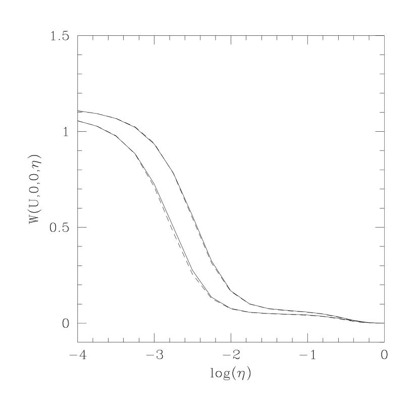
Figure 5: Solid lines show the correlation as a function of wavelength difference $\eta$ for zero separation ($r=0$) and zero source size ($r_{s}=0$) as calculated numerically. Dashed lines show the corresponding fitting function. Top Left: $\log(U)=-0.25,~{}-0.5,~{}-0.75,~{}-1.0$ (from above). Top Right: $\log(U)=0.5,~{}0.25,~{}0$ (from above). Bottom Left: $\log(U)=0.75,~{}1.0,~{}1.25,~{}1.5$ (from above). Bottom Right: $\log(U)=1.75,~{}2.0$ (from above).

Figure 3 shows that the flux correlation decays with increasing lag. The decay is described by a single lengthscale when $U$ is less than a few (weak scattering regime), whereas the decay occurs on two distinct lengthscales for larger values of $U$ (strong scattering). In the latter regime, the shorter of the two scales is the diffractive scale and the longer is the refractive scale (see Rickett 1990; Narayan 1993; for a review of the underlying physics of diffractive and refractive scintillation), and the ratio of the two scales increases with inreasing $U$ as $U^{6/5}$. The fluctuation power on the diffractive scale remains large for all values of $U$, whereas that on the refractive scale decays with increasing $U$. All of these properties are well-known and asymptotic results are available in the limit of both very large and very small $U$. The fitting function we have developed handles the asymptotic regimes well, but more importantly, it also models the analytically intractable regime corresponding to $U\sim 1-10$ quite satisfactorily. The most serious qualitative discrepancy is that the fitting function gives a positive value of the correlation for all lags, whereas the numerically computed correlation sometimes goes negative, especially for $U\sim 1$ (e.g., the top two panels of Fig. 3; see also Figs. 6, 7). More pronounced negative “overshoot” is seen in scintillation of some extragalactic intra-day variables and has been interpreted as evidence for anisotropic scattering(Rickett, 2002; Bignall et al., 2003).

Figure 4 shows the dependence of the flux correlation as a function of the source size $r_{s}$, and Figure 5 shows the dependence of the cross-correlation as a function of the dimensionless frequency difference $\eta$. Once again, the results clearly indicate the transition from a single scale in weak scattering to two scales in strong scattering. The fitting function does a remarkably good job for all values of $U$ and all choices of $r_{s}$ and $\eta$.

Figures 6, 7, 8 show the dependence of $W(U,r,r_{s},\eta)$ as a function of pairs of the three variables, $r$, $r_{s}$, $\eta$, keeping the third variable fixed at zero. These two-dimensional correlations are relatively less well explored in the literature, even in the asymptotic regimes, but our results are generally consistent with previous work wherever a comparison is possible. The behavior of $W(U,r,r_{s},0)$ in Figure 6 is easy to understand. With increasing source size, the fluctuations are progressively smoothed, so the fluctuation amplitude decreases and the scale of the fluctuations increases, just as one would expect. The dependences in Figures 7 and 8 are less obvious. With increasing frequency difference $\eta$, the decay scale of the correlation increases both as a function of $r$ (Fig. 7) and as a function of $r_{s}$ (Fig. 8); this is especially obvious in the plots for weak scintillation and strong diffractive scintillation. Equivalently, the decorrelation bandwidth increases with increasing $r$ and/or $r_{s}$. Chashei & Shishov (1976) showed such a dependence for strong diffractive scintillation for the particular case of a “square law” spectrum, $\alpha=2$. No analytical results have been reported for a Kolmogorov spectrum $\alpha=5/3$, but we see from our numerical work that the overall behavior is similar. In any case, Figures 6, 7 and 8 show that the fitting function reproduces the exact numerical results quite well for all values of $U$ and choices of $r$, $r_{s}$, $\eta$.

The behavior of flux scintillation in the $r-\eta$ plane has gained prominence in recent years as a result of the discovery of parabolic “arcs” and “arclets” in the so-called secondary spectrum (Stinebring et al., 2001; Cordes et al., 2005). Appendix C develops a rudimentary analytical theory of arcs that is valid in the two asymptotic regimes $U\ll 1$ and $U\gg 1$. The discussion there complements the more detailed physical approach taken by Cordes et al. (2005). The behavior of arcs in the transition regime $U\sim$ few, and in the presence of anisotropic turbulence, deserves further analytical and numerical study, but it is beyond the scope of this work. Researchers interested in arcs should be warned that our fitting functions were not designed with arcs in mind.

Figure 6: Solid lines show the numerically calculated correlation as a function of separation $r$ for a series of values of $r_{s}$, for $\eta=0$. In each panel, from above, the curves correspond to $r_{s}=0,~{}10^{-2},~{}10^{-1.5},~{}10^{-1},~{}10^{-0.5},~{}1,~{}10^{0.5},~{}10^{1},~{}10^{1.5},~{}10^{2}$. The dashed lines show the fitting function. Top Left: $U=1$. Top Right: $U=3.162$. Bottom Left: $U=10$. Bottom Right: $U=31.62$.

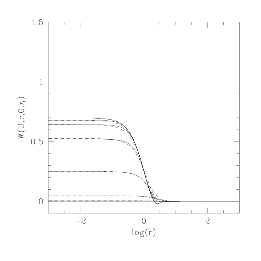
Figure 7: Solid lines show the numerically calculated correlation as a function of separation $r$ for a series of values of $\zeta$ (see eq. 27 for the definition), for $r_{s}=0$. In each panel, from above, the curves correspond to $\zeta=0,~{}10^{-2},~{}10^{-1.5},~{}10^{-1},~{}10^{-0.5},~{}1,~{}10^{0.5},~{}10$. The dashed lines show the fitting function. Top Left: $U=1$. Top Right: $U=3.162$. Bottom Left: $U=10$. Bottom Right: $U=31.62$.

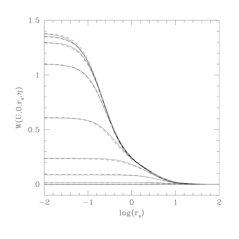
Figure 8: Solid lines show the correlation as a function of source size $r_{s}$ for a series of values of $\zeta$, for $r=0$. In each panel, from above, the curves correspond to $\zeta=0,~{}10^{-2},~{}10^{-1.5},~{}10^{-1},~{}10^{-0.5},~{}1,~{}10^{0.5},~{}10$. The dashed lines show the fitting function. Top Left: $U=1$. Top Right: $U=3.162$. Bottom Left: $U=10$. Bottom Right: $U=31.62$.

We have also compared the fitting function with the numerical results on $W(U,r,r_{s},\eta)$ for the case when all three variables, $r$, $r_{s}$, $\eta$, are varied, but we do not show the corresponding plots. By comparing the fitting function and the numerical results over an extensive grid of values of $U$, $r$, $r_{s}$ and $\eta$, we find that the maximum error in this four-dimensional space for a gaussian source is 0.047. The maximum error is larger for a tophat source, $\sim 0.06$, perhaps because the simplification of replacing the two source sizes $r_{s1}$ and $r_{s2}$ with a single effective size $r_{s}$ (eq. 18) is less well motivated in that case.

4.5 Logic Behind the Fitting Function

Although the fitting function described in the previous subsections was obtained to a large extent by a combination of intuition and trial-and-error, we tried to draw on analytical clues from Appendix B wherever possible.

Consider first $W_{0}(U)$. Equation (B.1) shows that in the limit of very weak scattering ($U\ll 1$) the flux variations have a mean square amplitude equal to $0.7729U$; the first term in the fitting function (21) is designed to satisfy this limit. Similarly, for very strong scattering ($U\gg 1$), equation (B11) shows that the refractive fluctuations have an amplitude $0.2380U^{-0.4}$ while equation (B14) indicates that the diffractive fluctuations have amplitude $1+0.2380U^{-0.4}$. Thus, the total mean square flux variations is equal to $1+0.4760U^{-0.4}$, which is ensured by the second term in equation (21) when $U\gg 1$. Also, we see that the diffractive fluctuations have a baseline amplitude of unity and that the excess fluctuations above unity are divided equally between diffractive and refractive fluctuations. This is the motivatation behind the particular split used in equation (38). The particular functional form that we have chosen in equation (21) to interpolate between the weak and strong scattering limits is completely arbitrary. In fact, it is easy to find other forms that model the transition region around $U\sim 1$ equally well.

Consider next the flux correlation as a function of separation $r$, for a point source ($r_{s}=0$) and zero wavelength difference ($\eta=0$). Equation (B13) shows that, for diffractive scintillation in the strong scattering regime with $\alpha=5/3$, the correlation varies as $\exp(-Ur^{5/3})$. When $r_{s}=\eta=0$ and $U\gg 1$, the parameter $R_{1}$ in equation (24) tends to $R_{5}$ in equation (40), whose leading term is proportional to $U^{-3/5}$. Thus, the $r$-dependence of the fitting function has the correct functional form. Unfortunately, the analytical result (B4) does not give a very convenient expression for $F_{r}$ in the weak scattering limit. However, since we require the fitting function to vary smoothly across the transition from strong diffractive to weak scattering, we use the same functional form (24) for both regimes. Similarly, the expression (B9) does not provide a useful approximation for the factor $F_{r,r}$ for strong refractive scintillation. By numerical experimentation we determined that $F_{r,r}$ cuts off more rapidly compared to $F_{r}$; we chose the index in (41) to be 7/3 out of a sense of “symmetry.”

Appendix B.3 discusses some asymptotic results for a finite source size. For large source size, the flux correlation is shown to decline as a power law in $r_{s}$, though with a different index in the different regimes. In refractive scintillation, the decline is described by $W\propto(r_{s}/r_{\rm ref})^{-7/3}$ (eq. B24 for $\alpha=5/3$) and this is hardwired into the fitting function via equation (42). The situation in the case of weak and strong diffractive scintillation is more complicated. The former has a scaling $W\propto r_{s}^{-7/3}$ (eq. B23) and the latter $W\propto(r_{s}/r_{\rm diff})^{-\beta}$ with $\beta<2$ (eq. B26). The two indices are thus different. However, we have required our fitting function to have a common set of scalings for weak and diffractive scintillation. (This is in the interests of simplicity and for smoothness across $U=U_{0}$). Because of this, we allowed the index on $(r_{s}/R_{2})$ in equation (25) to be a free parameter and adjusted it to give the best overall fit to the numerical data; this resulted in a value for the index of 1.81.

Finally, consider the correlation as a function of the parameter $\eta$ for $r=r_{s}=0$. First, notice that $\eta$ is defined such that it is equal to $\Delta\lambda/\lambda$ when the two wavelengths are close to each other, but it tends to unity as the wavelengths differ by an arbitrarily large amount. Because of the latter property, we have found it more convenient to use the modified parameter $\zeta$ defined in equation (27) in the fitting function. This parameter is equal to $\eta$ when $\eta\ll 1$, but it is proportional to the wavelength ratio $\lambda_{2}/\lambda_{1}$ as $\eta\to 1$.

In weak scattering and when $\eta,~{}\zeta\ll 1$, equation (B.1) shows that the correlation varies as $1-\eta^{5/6}$, i.e., roughly as $(1+\zeta^{5/6})^{-1}$. The functional form chosen for $F_{\eta}$ in equation (26) is designed to satisfy this limiting result (note that $a_{1}$ tends to a constant when $U\ll 1$). In the strong diffractive regime and in the limit of large $\eta$ (large compared to the decorrelation bandwidth but still small compared to unity), equation (B20) shows that the correlation declines as $\eta^{-2}U^{-2.4}$. This asymptotic dependence is ensured by the term $a_{2}(U)\zeta^{2}$ in equation (26). Finally, in the strong refractive regime, equation (B11) shows that the correlation varies as $1-\eta^{2}$ for small $\eta$. This is taken care of by the term $a_{4}(U)\zeta^{2}$ in equation (43), where we note that $a_{4}$ tends to a constant in the limit when $U\gg 1$.

While we have tried to respect asymptotic results for $U\ll 1$ and $U\gg 1$ to the extent possible, our primary interest is the regime in between where $U$ is neither very small nor very large. We have picked functional forms for the various terms in the fitting function such that they go smoothly between the two limits and agree as closely as possible with the numerical results. This is relatively easy to achieve when only one of the three parameters, $r$, $r_{s}$, $\eta$, is varied and the other two are set to zero (see the results shown in Figs. 3, 4, 5). However, we are also interested in variations of two (e.g., the arc phenomenon, Appendix C) or even three of these parameters simultaneously. Finding a reasonable fitting function to handle these regimes is more challenging. The particular function described in §4.2 and §4.3 could doubtless be improved, but it appears to fit the numerical results adequately over the entire parameter range of interest.

5 Summary

We provide in §4 of this paper a fitting function for a fairly general correlation, $W(U,r,r_{s},\eta)$, that describes the statistics of flux scintillations of compact radio sources. The function has been optimized for two source shapes, gaussian and tophat; the latter may be appropriate for gamma-ray burst afterglows (Sari 1998). We also allow for different source sizes and observation frequencies for the two flux measurements being correlated, which may again be useful for interpreting afterglow observations.

We have not specifically allowed for the finite integration time or finite bandwidth over which each flux measurement is made. Finite integration time causes any given flux correlation to correspond not to a single value of $r$ but to a range of values, i.e., $W(U,r,r_{s},\eta)$ is smeared in $r$ by a convolution. Similarly, finite bandwidth leads to smearing in $\eta$. These effects can be modeled by convolving the fitting function with the appropriate broadening functions in $r$ and $\eta$. Alternatively, they could be incorporated directly into the fitting function itself through additional factors (we have not attempted this here). In practice, with current technological limits, finite bandwidth is unlikely to be important in the regimes of weak or moderate scattering ($U\lesssim$ a few).

The results we have presented are for a single thin scattering screen. This is probably a reasonable model since the scattering regions in the interstellar medium tends to be clumpy. Therefore, the scattering is dominated by one or at most a few distinct screens. The model is also specific to a Kolmogorov spectrum of fluctuations in the scattering medium. This again is not unreasonable (e.g., Armstrong et al. 1981), although Boldyrev & Gwinn (2003) have recently challenged the usual assumption, which we have adopted, that the statistics of these fluctuations are gaussian.

The most serious simplifying assumption in this work is that we have taken the scattering to be isotropic, so that the scintillation correlation function depends on separation $r$ but not on the particular direction of $r$ transverse to the line-of-sight. A number of observations (e.g., Wilkinson et al. 1994; Dennett-Thorpe & de Bruyn 2003; and references therein) have shown that the scattering irregularities in the interstellar medium are anisotropic, presumably because blobs are elongated parallel to the local magnetic field. It would be useful to generalize the work described here to include anisotropy.

Appendix A Derivation of the flux correlation integral

The goal of this appendix is to derive the expression (A4) for the fourth-order coherence function in the special case that the points coincide in two pairs, so that it reduces to a flux correlation. Codona et al. (1986) have given a similar result for frequency-independent refractive fluctuations, e.g. atmospheric rather than interstellar turbulence. GN89 addressed the plasma case but assumed small frequency differences, an approximation that is not made here.

With ${\bf b}=0$, eq. (2.5.4) of GN89 becomes

$$\Gamma_{4}({\bf 0};{\bf r};\nu_{1},\nu_{2}) = \frac{1}{(\lambda_{1}\lambda_{2}z^{2})^{2}}\int d{\bf x}_{1}\int d{\bf x}_{2}\int d{\bf x}_{3}\int d{\bf x}_{4}$$ (A1)

$$\exp\left\{i\pi\left[\frac{{\bf x}_{1}^{2}-{\bf x}_{3}^{2}}{\lambda_{1}z}-\frac{({\bf x}_{2}-{\bf r})^{2}-({\bf x}_{4}-{\bf r})^{2}}{\lambda_{2}z}\right]\right\}$$

$$\exp\left\{-\frac{1}{2}\left\langle\phi({\bf x}_{1},\lambda_{1})-\phi({\bf x}_{3},\lambda_{1})-\phi({\bf x}_{2},\lambda_{2})+\phi({\bf x}_{4},\lambda_{2})\right\rangle\right\}.$$

Here $\lambda=c/\nu$ and $z$ is the effective distance to the thin screen, which impresses a phase shift $\phi({\bf x},\lambda)$ on rays of wavelength $\lambda$ that strike the screen at ${\bf x}$. The screen is parallel to the observer’s plane but separated from it by distance $z_{\rm screen}$, while $z\equiv(z_{\rm screen}^{-1}+z_{\rm source}^{-1})^{-1}$, where $z_{\rm source}$ is the distance from the screen to the source. Since $\phi$ involves the departure of the refractive index from unity due to free electrons all along the path of propagation, we assume that the $\phi\propto\lambda$. Also, $\phi({\bf x},\lambda)$ is proportional to the column density of electrons, which is stochastic. The mean-square phase differences impressed upon parallel paths meeting the screen at ${\bf x}_{1}$ and ${\bf x}_{2}$ is

$$D({\bf x}_{1}-{\bf x}_{2};\lambda) \equiv \left\langle\left[\phi({\bf x}_{1},\lambda)-\phi({\bf x}_{2},\lambda)\right]^{2}\right\rangle$$

$$D({\bf x}_{1}-{\bf x}_{2};\lambda^{\prime}) = \left(\frac{\lambda^{\prime}}{\lambda}\right)^{2}D({\bf x}_{1}-{\bf x}_{2};\lambda)\,,$$ (A2)

where $\langle\ldots\rangle$ is an appropriate statistical average. Let $\bar{\lambda}\equiv(\lambda_{1}\lambda_{2})^{1/2}$, $\rho\equiv(\lambda_{2}/\lambda_{1})^{1/2}$, $\phi_{i}\equiv\phi({\bf x}_{i},\bar{\lambda})$, and $D_{ij}\equiv D({\bf x}_{i}-{\bf x}_{j},\bar{\lambda})$. Since $\langle\phi_{i}\phi_{j}\rangle=\sigma^{2}-\frac{1}{2}D_{ij}$, where $\sigma^{2}$ is the variance of $\phi$, the second exponential in eq. (A1) is

$$\exp\left\{-\frac{1}{2}\left[\rho^{-2}D_{13}+\rho^{2}D_{24}+D_{12}+D_{34}-D_{14}-D_{23}\right]\right\}.$$ (A3)

Next, multiply (A1) by

$$\int d{\bf c}~{}\delta\left({\bf c}-\frac{1}{4}\sum_{i=1}^{4}{\bf x}_{i}\right)=1.$$

Then shift variables ${\bf x}\to{\bf x}+{\bf c}$, which has no effect on (A3) but multiplies the first exponential in (A1) by

$$\exp\left[2\pi i{\bf c\cdot}\left(\frac{{\bf x}_{1}-{\bf x}_{3}}{\lambda_{1}z}-\frac{{\bf x}_{2}-{\bf x}_{4}}{\lambda_{2}z}\right)\right]\,.$$

After integration over ${\bf c}$, the net effect of these steps is to insert the delta functions

$$\delta\left(\frac{{\bf x}_{1}+{\bf x}_{2}+{\bf x}_{3}+{\bf x}_{4}}{4}\right)\,\delta\left(\frac{{\bf x}_{1}-{\bf x}_{3}}{\lambda_{1}z}-\frac{{\bf x}_{2}-{\bf x}_{4}}{\lambda_{2}z}\right)$$

into the integrand of (A1). So, only two combinations of the ${\bf x}$s are independent. It is convenient to choose these as

$${\bf q} \equiv \frac{1}{2}(1+\rho^{2})({\bf x}_{1}-{\bf x}_{3})~{}=~{}\frac{1}{2}(1+\rho^{-2})({\bf x}_{2}-{\bf x}_{4})$$

$${\bf s} \equiv \frac{1}{2}({\bf x}_{1}+{\bf x}_{3}-{\bf x}_{2}-{\bf x}_{4})\,,$$

because the Fresnel (i.e. first) exponential in (A1) then becomes

$$\exp\left[\frac{4\pi i}{(\lambda_{1}+\lambda_{2})z}{\bf q\cdot}({\bf s}+{\bf r})\right]$$

After integrating out the two delta functions and expressing the remaining integrals in terms of ${\bf q}$ & ${\bf s}$, one has

$$\Gamma_{4}({\bf 0};{\bf r};\nu_{1},\nu_{2}) = \frac{1}{(2\pi r_{\rm F}^{2})^{2}}\int\,d{\bf q}\exp\left(\frac{i{\bf r}\cdot{\bf q}}{r_{\rm F}^{2}}\right)\int d{\bf s}\,\exp\left(\frac{i{\bf q}\cdot{\bf s}}{r_{\rm F}^{2}}\right)$$ (A4)

$$\times \exp\left\{-\frac{1}{2}\left[\frac{1-\eta}{1+\eta}D((1-\eta){\bf q})+\frac{1+\eta}{1-\eta}D((1+\eta){\bf q})\right.\right.$$

$$\qquad\left.\left.\vphantom{\frac{1-\eta}{1+\eta}}+D({\bf s}-\eta{\bf q})+D({\bf s}+\eta{\bf q})-D({\bf s}-{\bf q})-D({\bf s}+{\bf q})\right]\right\}\,,$$

in which the structure functions (the $D$s) are evaluated at the geometric mean $\sqrt{\lambda_{1}\lambda_{2}}$ of the two wavelengths, whereas the Fresnel scale is defined with the arithmetic mean, eq. (4), and $\eta$ is the dimensionless frequency difference (5). Equation (A4) agrees with eqs. (17)-(18) of Codona et al. (1986), apart from what appear to be minor typographical errors and for changes to allow for the $\lambda^{2}$ dependence of the plasma refractive index.

Appendix B Asymptotic Results for the Flux Correlation

The bulk of this Appendix is devoted to analytical results for the flux correlation in various asymptotic regimes. Since the following presentation is rather dense, we begin with an index to the main results:

• Weak scintillation ($U\ll 1$): Eqs. (B4), (B.1).

• Strong refractive scintillation: Eqs. (B8)-(B11).

• Strong diffractive scintillation:

  • Total flux variance (i.e., ${\bf r}=0=\eta$): Eq. (B15)

  • Diffractive correlation at $r=0$ but $\eta\neq 0$: Eqs. (B18)-(B19).

  • Diffractive correlation at $r\neq 0$ & $\eta\gg U^{-2/\alpha}$: Eq. (B21).

§B.3 discusses the effect of a finite source size.

B.1 Weak scattering ($U\ll 1$)

The idea here is to take $\exp(-G/2)\approx 1-G/2$ in (8). This is justified because on the one hand, $|G|\lesssim O\left(Uq^{\alpha}\right)$ since $G\to 0$ as $s/q\to\infty$; and on the other hand, $Uq^{\alpha}\ll 1$ unless $q\gg 1$, in which case the rapidly oscillating factor $\exp(i{\bf q}\cdot{\bf s})$ suppresses the integral anyway:

$$\widetilde{W}({\bf q},\eta) \approx (2\pi)^{2}\delta({\bf q})~{}-~{}\frac{1}{2}U\int d{\bf s}\,e^{i{\bf q}\cdot{\bf s}}\left[\left|{\bf s}-\eta{\bf q}\right|^{\alpha}+\left|{\bf s}+\eta{\bf q}\right|^{\alpha}-\left|{\bf s}-{\bf q}\right|^{\alpha}-\left|{\bf s}+{\bf q}\right|^{\alpha}\right]$$ (B1)

$$~{}+~{}O(U^{2}).$$

The delta function simply reflects the fact that the mean flux is nonzero. In the remaining integral, each term has the form

$$\int d{\bf s}\,e^{i{\bf q}\cdot{\bf s}}\left|{\bf s}-{\bf a}\right|^{\alpha}=e^{i{\bf q}\cdot{\bf a}}\int d{\bf t}\,e^{i{\bf q}\cdot{\bf t}}\left|{\bf t}\right|^{\alpha}=2\pi e^{i{\bf q}\cdot{\bf a}}\int\limits_{0}^{\infty}t^{\alpha+1}J_{0}(qt)\,dt.$$

The final integral is divergent, but for $-1<\alpha<-1/2$ it would be (Abramowitz & Stegun, 1972, §11.4.16)

$$2\pi\int\limits_{0}^{\infty}t^{\alpha+1}J_{0}(qt)\,dt=-2^{\alpha+2}\Gamma^{2}(\alpha/2+1)\sin(\pi\alpha/2)q^{-\alpha-2}.$$ (B2)

We assume that this formula can in fact be used for all $\alpha$. Presumably the result could be justified by inserting a slowly decreasing smooth function of $s$ into the original integrand (8), for example $\exp(-\epsilon s^{2})$, and then taking the limit $\epsilon\to 0$. Such a convergence factor is implicit in the Fresnel approximation to physical optics since the phase screen is actually only a local approximation to a closed surface enveloping the observer and therefore has finite area. The final result is

$$\widetilde{W}({\bf q};\eta,U) \approx 2^{\alpha+2}\Gamma^{2}(\alpha/2+1)\sin(\pi\alpha/2)\,Uq^{-\alpha-2}\left[\cos(\eta q^{2})-\cos(q^{2})\right]$$ (B3)

$$+O(U^{2}),\qquad q\neq 0.$$

The flux correlation (7) works out to

$$W({\bf r};\eta,U) \approx 1+~{}2^{\alpha}\Gamma(\alpha/2+1)U\left[f(1,r)-f(\eta,r)\right]~{}+O(U^{2}),$$ (B4)

$$\mbox{where}~{}~{}f(\eta,r) \equiv \eta^{\alpha/2}\Re\left[e^{i\pi\alpha/4}M(-\alpha/2,1,ir^{2}/4\eta)\right]\,;$$

$$M(a,1,z) \equiv \sum\limits_{n=0}^{\infty}\frac{\Gamma(a+n)}{\Gamma(a)(n!)^{2}}\,z^{n},$$

is a confluent hypergeometric function (Abramowitz & Stegun, 1972), and $\Re$ denotes the real part. The series for $M$ converges at all $z$. The “$1+$” on the first line above represents the square of the mean flux; we write $\Delta W\equiv W-1$. The correlation at zero spatial separation is particularly simple:

$$\Delta W({\bf 0};\eta,U) \approx 2^{\alpha}\Gamma(\alpha/2+1)\cos(\pi\alpha/4)\left(1-\eta^{\alpha/2}\right)U~{}+~{}O(U^{2})$$

$$\to 0.7729\left(1-\eta^{\alpha/2}\right)U~{}+~{}O(U^{2})~{}~{}\mbox{at}~{}\alpha=5/3.$$

B.2 Strong scattering

B.2.1 Refractive regime

Even when $U\gg 1$, the weak-scattering formula (B3) is valid if $q\ll q_{\rm ref}$,

$$q_{\rm ref}\equiv U^{-1/\alpha}.$$ (B6)

Actually, one can extend the result to $q\sim q_{\rm ref}$ as follows. The integral over ${\bf s}$ is dominated by $s\sim 1/q$, where the oscillating exponential cuts it off; in this range,

$$G\approx(1-\eta^{2})Uq^{\alpha}\left[\alpha+\alpha(\alpha-2)\cos^{2}\theta\right]\left(\frac{q}{s}\right)^{2-\alpha}~{}+~{}O\left(Uq^{4}s^{\alpha-4}\right),\qquad{s\gg q}\,,$$ (B7)

where $\cos\theta$ is the angle between ${\bf q}$ and ${\bf s}$. Since we assume $\alpha<2$, it follows that $G\ll Uq^{\alpha}\lesssim 1$, so that we may again evaluate (8) by expanding $\exp(-G/2)$ to first order in its argument. In contrast to the previous section, however, we retain the prefactor $\exp(-F/2)$ because it cuts off the refractive spectrum sharply at $q\sim q_{\rm ref}$:

$$\widetilde{W}_{\rm ref}({\bf q})\approx 2^{\alpha+1}\sin(\pi\alpha/2)\Gamma^{\,2}(\alpha/2+1)(1-\eta^{2})Uq^{2-\alpha}\exp[-F(q;\eta,U)/2],\qquad q\lesssim q_{\rm ref}.$$ (B8)

Integrating over the direction of ${\bf q}$ so that $\exp({\bf q}\cdot{\bf s})\to 2\pi J_{0}(qr)$, expressing $J_{0}(z)$ by its power series, and integrating term by term, one finds

$$\Delta W_{\rm ref}(r;\eta,U) \approx \frac{2^{\alpha-1}\Gamma(\alpha/2\,+1)\Gamma(4/\alpha\,-1)}{\Gamma(-\alpha/2\,+1)}\,\frac{(1-\eta^{2})U}{U_{\eta}}\,U_{\eta}^{-2(2-\alpha)/\alpha}$$ (B9)

$$\times \sum\limits_{n=0}^{\infty}\frac{\Gamma[(4+2n)/\alpha\,-1]}{\Gamma(4/\alpha-1)\,(n!)^{2}}\,\left(-\frac{r^{2}}{4U_{\eta}^{2/\alpha}}\right)^{n}.$$

We have introduced the abbreviation

$$U_{\eta}\equiv\frac{(1-\eta)^{\alpha+2}+(1+\eta)^{\alpha+2}}{2(1-\eta^{2})}\,U\,.$$ (B10)

Unfortunately the power series on the second line of (B9) is not any sort of hypergeometric function, but it converges for all $r$ if $\alpha>1$. In particular,

$$\Delta W_{\rm ref}(0;\eta,U)\approx 0.2380(1-\eta^{2})\frac{U}{U_{\eta}}\,U_{\eta}^{-2/5},\qquad\alpha=5/3.$$ (B11)

B.2.2 Diffractive regime

If the dimensionless frequency difference $\eta\lesssim U^{-2/\alpha}$, there is also a diffractive contribution to $W$ and $\widetilde{W}$. This comes from $q\gg q_{\rm ref}\sim s$ in the integral (8). Consider first $\eta=0$. Then

$$\frac{1}{2}(F+G)\approx Us^{\alpha}\,\left[1~{}+~{}O(s/q)^{\alpha-2}\right].$$

Keeping only the leading order term gives

$$\Delta W_{\rm diff}({\bf r};0,U)\approx\int\frac{d{\bf q}}{(2\pi)^{2}}e^{i{\bf r}\cdot{\bf q}}\int d{\bf s}\,e^{i{\bf q}\cdot{\bf s}}\exp\left(-Us^{\alpha}\right).$$ (B12)

But this is just a Fourier transform followed by its inverse. So to leading order,

$$\Delta W_{\rm diff}({\bf r};0,U)\approx\exp\left(-Ur^{\alpha}\right).$$ (B13)

We have written $\Delta W_{\rm diff}$ rather than $W$ because (B12) applies only to $q\gg q_{\rm ref}$ and therefore omits both the refractive contribution (B9) and the square of the mean flux, both of which stem from from $q\lesssim q_{\rm ref}$. The total flux correlation is $1+\Delta W_{\rm ref}+\Delta W_{\rm diff}$.

At the current level of approximation (B13), the contribution of diffractive scintillation to the flux variance (the correlation at ${\bf r}=0$) is simply unity, i.e., equal to the square of the mean flux, whereas the contribution from refraction scales as $U^{-2(2-\alpha)/\alpha}$. We can refine the diffractive variance by the following trick. With ${\bf r}=0$ and $\eta=0$, the integral (7) is symmetrical in ${\bf s}$ & ${\bf q}$:

$$W({\bf 0};0,U)=\frac{1}{(2\pi)^{2}}\int d{\bf q}\int d{\bf s}\,e^{i{\bf q}\cdot{\bf s}}\exp\left\{U\left[\frac{1}{2}|{\bf s}+{\bf q}|^{\alpha}+\frac{1}{2}|{\bf s}-{\bf q}|^{\alpha}-s^{\alpha}-q^{\alpha}\right]\right\}\,.$$

According to §B.2.1, the contribution from $s\gg q$ is $1+\Delta W_{\rm ref}({\bf 0};0,U)$. Symmetry demands that the contribution from $s\ll q$ must be the same:

$$\Delta W_{\rm diff}({\bf 0};0,U)\approx~{}1+\Delta W_{\rm ref}({\bf 0};0,U)\,,$$ (B14)

and therefore the total flux variance in a very narrow frequency band is

$$\frac{\langle F^{2}\rangle}{\langle F\rangle^{2}}~{}-1~{}=~{}1+2\Delta W_{\rm ref}({\bf 0};0,U)\,.$$ (B15)

The factor of two reflects equal contributions from the refractive ($s\gg q$) and diffractive ($s\ll q$) regimes; but this symmetry should not obscure the fact that the diffractive and refractive contributions decorrelate on widely different lengthscales $r_{\rm diff}\sim U^{-1/\alpha}$ [eq. (B13)] and $r_{\rm ref}\sim U^{+1/\alpha}$ [eq. (B9)], respectively.

Let us now consider nonzero frequency differences, $\eta\neq 0$. The most sensitive terms are the structure functions $U|{\bf s}\pm\eta{\bf q}|^{\alpha}$; other appearances of $\eta$ are smaller by at least $O(\eta^{2-\alpha})$:

$$\Delta W_{\rm diff}({\bf r};\eta,U)\approx\int\frac{d{\bf q}}{(2\pi)^{2}}e^{i{\bf r}\cdot{\bf q}}\int d{\bf s}\,e^{i{\bf q}\cdot{\bf s}}\exp\left[-\frac{1}{2}U\left(|{\bf s}+\eta{\bf q}|^{\alpha}+|{\bf s}-\eta{\bf q}|^{\alpha}\right)\right].$$ (B16)

This reduces to (B12) at $\eta=0$. With the change of variables

$${\bf s} = \left(\frac{\eta}{2}\right)^{1/2}({\bf u}+{\bf v}),\qquad{\bf q}=\left(\frac{1}{2\eta}\right)^{1/2}({\bf u}-{\bf v}),$$

$${\bf r} = (2\eta)^{1/2}{\bf\rho},\qquad\mbox{and}\quad V=\frac{1}{2}(2\eta)^{\alpha/2}U,$$ (B17)

the double vector integral can be factored into the product of independent integrations over ${\bf u}$ and ${\bf v}$ that are complex conjugates:

$$\Delta W_{\rm diff}({\bf r};\eta,U) \approx \left|f(\rho,V)\right|^{2},$$ (B18)

$$\mbox{where}~{}~{}f(\rho,V) \equiv \int\frac{d{\bf u}}{2\pi}e^{-i{\bf\rho}\cdot{\bf u}-iu^{2}/2-Vu^{\alpha}}~{}=~{}\int\limits_{0}^{\infty}J_{0}(\rho u)\exp\left(-iu^{2}/2-Vu^{\alpha}\right)\,udu.$$

[The object $f(\rho,V)$ is equivalent to the two-frequency, two-position second moment of the electric field given by eq. (50) of Lambert & Rickett (1999), who also cite previous work on the latter quantity. It is well known that fourth moments of the field, such as $W$, can usually be approximated by squares of second moments in very strong scattering (cf. e.g. Codona et al., 1986).] The monochromatic limit $\eta\to 0$ is recovered by taking $V\to 0$ while keeping $(2V)^{1/\alpha}\rho=U^{1/\alpha}r$ constant. We have no general closed-form expression for $f(\rho,V)$, but at $r=0$,

$$f(0,V) = -i\sum\limits_{n=0}^{\infty}\frac{\Gamma(n\alpha/2+1)}{n!}\left(-e^{-i\pi\alpha/4}2^{\alpha-1}\eta^{\alpha/2}U\right)^{n}\,$$ (B19)

$$\sim \frac{2^{2/\alpha}}{2\alpha\eta U^{2/\alpha}}\sum\limits_{n\geq 0}\frac{\Gamma[2(n+1)/\alpha]}{n!}\left(-\frac{i}{2}V^{-2/\alpha}\right)^{n}\,.$$

Looking at the first two terms of this sum, one sees that for small $\eta$, the intensity decorrelates as

$$W({\bf 0};0,0)-W({\bf 0};\eta,0)\approx 2^{\alpha}\Gamma\left(\frac{\alpha+2}{2}\right)\cos\left(\frac{\pi\alpha}{4}\right)\eta^{\alpha/2}U$$

in agreement with eq. (21) of Shishov et al. (2003) if one assumes that the scattering, which they take to be distributed along the line of sight, is instead concentrated on a thin screen at distance $R/2$, and if the term $\cos\frac{n-2}{4\pi}$ should have read $\cos\frac{(n-2)\pi}{4}$ therein. The second sum in (B19) is asymptotic and shows that

$$\Delta W_{\rm diff}({\bf 0};\eta,U)\approx 2^{-4(\alpha-1)/\alpha}\Gamma^{\,2}(2/\alpha\,+1)\left(\eta U^{2/\alpha}\right)^{-2}\quad\mbox{if}~{}\eta\gg U^{-2/\alpha}.$$ (B20)

From either sum, one sees that the decorrelation bandwidth is $\eta\sim U^{-2/\alpha}=q_{\rm ref}^{2}$.

Let us now consider the dependence on spatial lag ${\bf r}$. For $\eta\lesssim q_{\rm ref}^{2}$, this is approximately the same as for $\eta=0$, eq. (B13). For $\eta\gg q_{\rm ref}^{2}$, the term $iu^{2}/2\ll Vu^{\alpha}$ in (B18) except where the integrand is negligibly small anyway. By omitting $iu^{2}/2$ from the exponential and rescaling the dummy variable $u\to V^{-1/\alpha}t$, one can obtain

$$\Delta W_{\rm diff}({\bf r};\eta,U) \approx \Delta W_{\rm diff}({\bf 0};\eta,U)\left|g\left[\frac{r}{2\eta(U/2)^{1/\alpha}}\right]\right|^{2},$$ (B21)

$$\mbox{where}~{}~{}g(z) = \frac{\alpha}{\Gamma(2/\alpha)}\int\limits_{0}^{\infty}J_{0}(zt)e^{-t^{\alpha}}\,tdt.$$

$$= \frac{1}{\Gamma(2/\alpha)}\sum\limits_{n=0}^{\infty}\frac{\Gamma[2(n+1)/\alpha]}{(n!)^{2}}\left(-\frac{z^{2}}{4}\right)^{n}\,.$$

[Mathematically $g(z)$, is essentially the same as the function $Q_{\rm PD}(\tau)$ given in eq. (54) of Lambert & Rickett (1999), but the latter is interpreted physically as a pulse-broadening profile at zero spatial lag.] To be consistent with the assumption $\eta\gg U^{-2/\alpha}$, one ought to use (B20) for $\Delta W_{\rm diff}({\bf 0};\eta,U)$ in the above formula, but one might want to use the more accurate value $|f(0,V)|^{2}$ as given by (B19) instead.

B.3 Finite Source Size

Equations (14)–(16) show how a finite source size modifies the flux correlation. For zero separation ($r=0$), for instance, we have

$$W(r=0,r_{s}\neq 0)\approx{1\over 2\pi}\int_{0}^{1/r_{s}}\widetilde{W}(q)qdq,$$ (B22)

where $r_{s}$ refers to the effective source defined in equation (18), and we have made use of the fact that the Hankel transform $\widetilde{S}(q)$ of a source with a finite size cuts off at $q\sim 1/r_{s}$. Using this result, we may estimate the effect of a finite source size in the different scattering regimes. In the following, we assume for simplicity that $r=\eta=0$.

In weak scattering, there is a reduction in the flux variations when the source size is greater than the Fresnel scale, i.e., $r_{s}>1$ in our units. Thus, the relevant range of $\widetilde{W}(q)$ for evaluating the integral in equation (B22) is $q<1/r_{s}\lesssim 1$. In this regime, $\widetilde{W}(q)\sim q^{2-\alpha}$ (see equation B3), and hence we obtain

$$W_{\rm weak}(r=0,r_{s},\eta=0)\propto r_{s}^{\alpha-4},\qquad r_{s}>1.$$ (B23)

In strong refractive scintillation, finite source effects are felt when the source size exceeds the refractive scale $r_{\rm ref}\sim 1/q_{\rm ref}$. In this regime again $\widetilde{W}(q)$ varies as $q^{2-\alpha}$ (see eq. B8), and so we obtain

$$W_{\rm ref}(r=0,r_{s},\eta=0)\propto(r_{s}/r_{\rm ref})^{\alpha-4},\qquad r_{s}>r_{\rm ref}.$$ (B24)

Finally consider strong diffractive scintillation. In the asymptotic limit of very strong scattering ($U\gg 1$), $\widetilde{W}(q)$ is constant ($\widetilde{W}(q)\sim q^{0}$, white noise) upto $q\sim q_{\rm diff}$ (e.g., Goodman & Narayan 1985). For a source size $r_{s}>r_{\rm diff}\sim 1/q_{\rm diff}$, this gives

$$W_{\rm diff}(r=0,r_{s},\eta=0)\propto(r_{s}/r_{\rm diff})^{-2},\qquad r_{s}>r_{\rm diff},~{}U\gg 1.$$ (B25)

However, unless $U$ is extremely large, the next order term in $\widetilde{W}(q)$ cannot be neglected, and it gives a correction that causes $\widetilde{W}(q)$ to decrease with increasing $q$ (e.g., see Fig. 1 of Goodman & Narayan 1985, where the decrease is apparent even for $U=10^{4}$). As a result, the scaling due to a finite source size is modified slightly to

$$W_{\rm diff}(r=0,r_{s},\eta=0)\propto(r_{s}/r_{\rm diff})^{-\beta},\qquad r_{s}>r_{\rm diff},~{}\beta<2,$$ (B26)

where the exact value of $\beta$ depends on $U$; $\beta$ is distinctly less than 2 when $U$ is not very large, but it tends to 2 as $U\to\infty$.

Appendix C Parabolic arcs in secondary spectra

The dynamical spectrum of a scintillating source is the flux correlation in a two-dimensional plane of time and frequency lag. Its Fourier transform with respect to both arguments is called the secondary spectrum $S_{2}(f_{\nu},f_{t})$. When the interesting range of frequencies is small compared to the mean frequency, $\Delta\nu\ll\nu$, and when the correspondence between spatial and temporal lags is governed by the transverse velocity ${\bf v}_{\perp}$ of line of sight, ${\bf r}={\bf v}_{\perp}t$, the secondary spectrum is related to the cross spectrum (8) by

$$S_{2}(f_{\nu},f_{t})=\frac{r_{\rm F}}{v_{\perp}}\int\frac{dq^{\prime}}{2\pi}\int\nu d\eta~{}\widetilde{W}\left(q_{t}\hat{\bf v}_{\perp}+q^{\prime}\hat{\bf e}^{\prime},\eta\right)e^{2\pi if_{\nu}\nu\eta}\,,$$ (C1)

in which $v_{\perp}\equiv|{\bf v}_{\perp}|$, and $\hat{\bf v}_{\perp}$ & $\hat{\bf e}^{\prime}$ are unit vectors on the sky parallel & perpendicular to ${\bf v}_{\perp}$, respectively, while $q_{t}\equiv 2\pi r_{\rm F}f_{t}/v_{\perp}$ is the component of the wavenumber parallel to the motion through the scintillation pattern. The Fresnel scale (4) appears here because $\widetilde{W}$ and ${\bf q}$ have been expressed in units where $r_{\rm F}=1$: that is, the physical wavenumber is $r_{\rm F}{\bf q}$. The integration over $q^{\prime}$ reduces the 2D cross-spectrum $\widetilde{W}$ to a 1D cross-spectrum.

Secondary spectra often show a concentration of power along parabolic ridges $f_{\nu}=\pm af_{t}^{2}$ (Stinebring et al., 2001). Cordes et al. (2005) have given a theoretical explanation of this phenomenon, according to which the coefficient $a=z\lambda^{2}/(cv_{\perp}^{2})$, where $z$ is the effective distance of the screen (1).

The existence of parabolic arcs in strong diffractive scattering can be demonstrated from equation (B16), which is equivalent to

$$\widetilde{W}_{\rm diff}({\bf q};\eta,U)\approx\int d{\bf s}\,e^{i{\bf q}\cdot{\bf s}}\exp\left[-\frac{1}{2}U\left(|{\bf s}+\eta{\bf q}|^{\alpha}+|{\bf s}-\eta{\bf q}|^{\alpha}\right)\right].$$ (C2)

This is a good approximation to the exact relations (8)-(10) when $\eta^{2}Uq^{\alpha}\ll 1$ (even though $Uq^{\alpha}$ may be large) so that the neglected terms in the exponential approximately cancel. For large $q$, the integral over ${\bf s}$ is dominated by the neighborhood of its branch points. The leading-order contribution from ${\bf s}\approx\eta{\bf q}$ can be obtained by setting $|{\bf s}+\eta{\bf q}|^{\alpha}\to|2\eta{\bf q}|^{\alpha}$ (because this part of the integrand remains smooth in that neighborhood) and then expanding the remaining exponential to first order in its argument; treating ${\bf s}\approx-\eta{\bf q}$ similarly, one has

$$\widetilde{W}_{\rm diff}({\bf q};\eta,U) \approx e^{-(U/2)|2\eta q|^{\alpha}}\left[\int d{\bf s}\,e^{i{\bf q}\cdot{\bf s}}\left(1-\frac{U}{2}|{\bf s}-\eta{\bf q}|^{\alpha}\right)~{}+~{}\int d{\bf s}\,e^{i{\bf q}\cdot{\bf s}}\left(1-\frac{U}{2}|{\bf s}+\eta{\bf q}|^{\alpha}\right)\right]$$

$$\approx 2(2\pi)^{2}\delta({\bf q})~{}+~{}K_{\alpha}Uq^{-\alpha-2}\,\cos(\eta q^{2})e^{-(U/2)|2\eta q|^{\alpha}}\,,$$

where $-K_{\alpha}$ is the coefficient of $q^{-\alpha-2}$ in eq. (B2). The delta function must be discarded since $q$ is large. When the remainder is used in (C1) to calculate the secondary spectrum, the exponential in $U|2\eta q|^{\alpha}$ can be replaced by unity if

$$f_{\nu}\gg\frac{r_{\rm F}}{\nu v_{\perp}}U^{1/\alpha}f_{t}\,,$$ (C3)

because the complex exponential will then effectively limit $\eta$ to small values:

$$S_{2}(f_{\nu},f_{t})\approx\frac{1}{2}K_{\alpha}U\frac{r_{F}\nu}{v_{\perp}}\int\frac{dq^{\prime}}{2\pi}\left(q_{t}^{2}+q^{\prime\,2}\right)^{-(\alpha+2)/2}\left[\delta\left(\nu f_{\nu}+\frac{q_{t}^{2}+q^{\prime\,2}}{2\pi}\right)~{}+~{}\delta\left(\nu f_{\nu}-\frac{q_{t}^{2}+q^{\prime\,2}}{2\pi}\right)\right].$$ (C4)

The parabolic arcs can now be recognized in the arguments of these delta functions, which are softened but not suppressed by the final integration over the transverse wavenumber:

$$S_{2}(f_{\nu},f_{t}) \approx (2\pi)^{-3/2}\left(\frac{2}{\pi}\right)^{\alpha/4}\Gamma^{2}\left(\frac{\alpha+2}{2}\right)\sin\left(\frac{\pi\alpha}{2}\right)U\frac{\sqrt{cz}}{v_{\perp}}$$ (C5)

$$\times ~{}\left(\frac{v_{\perp}^{2}}{\lambda zf_{t}^{2}}\right)^{(\alpha+2)/4}\left(|f_{\nu}|-af_{t}^{2}\right)^{-1/2}H(|f_{\nu}|-af_{t}^{2}).$$

Here $a=\lambda^{2}z/cv_{\perp}^{2}$ as before, and the Heaviside function keeps the argument of the square root positive. The Heaviside function cuts off the power abruptly for $|f_{t}|>(|f_{\nu}|/a)^{1/2}$, and the inverse square root concentrates power just inside this cutoff. Both observations and numerical simulations confirm this general behavior (Cordes et al., 2005), and this is the origin of the arcs. Plausibly the arcs would be more prominent if the electron-density spectrum were anisotropic with stronger scattering along $\hat{\bf v}_{\perp}$ than along $\hat{\bf e}^{\prime}$, because the integration (C4) would have less of a smearing effect. Presumably also, arcs should be more prominent when scattering is dominated by a thin “screen” rather than distributed along the line of sight, since integration over $z$ would further soften the final square root in eq. (C5). These points are made by Cordes et al. (2005).

In strong scattering ($U\gg 1$), the conditions for validity of the final result (C5) include not only eq. (C3) but also $q_{t}\equiv 2\pi f_{t}/v_{\perp}\gg U^{-1/\alpha}=q_{\rm diff}$ so that the integration over ${\bf s}$ is dominated by $s\ll q$. However, the same result obtains in weak scattering as well provided $2\pi f_{t}\gg v_{\perp}/r_{\rm F}$, since the same $\cos(\eta q^{2})$ term appears in eq. (B8) and gives rise to delta functions in the $\eta\to f_{\nu}$ transform of the 2D cross spectrum. In fact, regardless of the magnitude of the scintillation parameter $U$, it appears that the arcs are due to weak large-angle scattering by inhomogeneities smaller than those that are responsible for the main part of the scatter-broadened image (Cordes et al., 2005).

References

- Abramowitz & Stegun (1972) Abramowitz, M. & Stegun, I. A. 1972, Handbook of Mathematical Functions, New York: Dover.
- Armstrong et al. (1981) Armstrong, J. W., Cordes, J. M., & Rickett, B. J. 1981, Nature, 291, 561
- Bignall et al. (2003) Bignall, H. E. et al. 2003, ApJ, 585, 653
- Boldyrev & Gwinn (2003) Boldyrev, S. & Gwinn, C. 2003, ApJ, 584, 791
- Chashei & Shishov (1976) Chashei, I. V., & Shishov, V. I. 1976, Sov. Astron., 20, 13
- Codona et al. (1986) Codona, J. L., Creamer, D. B., Flatté, S. M., Frehlich, R. G., & Henyey, F. S. 1986, Radio Science, 21, 805
- Cordes et al. (1983) Cordes, J. M., Weisberg, J. M., & Boriakoff, V. 1983, ApJ, 268, 370
- Cordes et al. (2005) Cordes, J. M., Rickett, B. J., Stinebring, D. R., & Coles, W. A. 2005, astro-ph/0407072.
- Dennett-Thorpe & de Bruyn (2003) Dennett-Thorpe, J, & de Bruyn, A. G. 2003, A&A, 404, 113
- Frail et al. (1997) Frail, D. A., Kulkarni, S. R., Nicastro, L., Feroci, M., & Taylor, G. B. 1997, Nature, 389, 261
- Goodman (1997) Goodman, J. 1997, New Astr., 2, 449
- Goodman & Narayan (1985) Goodman, J. & Narayan, R. 1985, MNRAS, 214, 519
- Goodman & Narayan (1989) Goodman, J. & Narayan, R. 1989, MNRAS, 238, 995
- Gwinn et al. (1997) Gwinn, C. R., Ojeda, M. J., Britton, M. C., Reynolds, J. E., Jauncey, D. L., King, E. A., McCulloch, P. M., Lovell, J. E. J., et al. 1997, ApJ, 483, L53
- Hewish (1993) Hewish, A. 1993, in Pulsars as Physics Laboratories, eds R. D. Blandford, A. Hewish, A. G. Lyne, & L. Mestel, p167, Oxford Univ. Press
- Lambert & Rickett (1999) Lambert, H. C., & Rickett, B. J. 1999, ApJ, 517, 299
- Lovell et al. (2003) Lovell, J. E. J., Jauncey, D. L., Bignall, H. E., Kedziora-Chudczer, L., Macquart, J.-P., Rickett, B. J., & Tzioumis, A. K. 2003, AJ, 126, 1699
- Narayan (1993) Narayan, R. 1993, in Pulsars as Physics Laboratories, eds R. D. Blandford, A. Hewish, A. G. Lyne, & L. Mestel, p151, Oxford Univ. Press
- Rickett (1990) Rickett, B. J. 1990, ARA&A, 28, 561
- Rickett (2001) Rickett, B. J. 2001, Ap&SS, 278, 5
- Rickett (2002) Rickett, B. J. 2002, Pub. Astron. Soc. Australia, 19, 100
- Rickett et al. (1995) Rickett, B. J., Quirrenbach, A., Wegner, R., Krichbaum, T. P., & Witzel, A. 1995, A&A, 293, 479
- Rickett et al. (2001) Rickett, B. J., Witzel, A., Kraus, A., Krichbaum, T. P., & Qian, S. J. 2001, ApJ, 550, L11
- Roberts & Ables (1982) Roberts, J. A., & Ables, J. G. 1982, MNRAS, 201, 1119
- Sari (1998) Sari, R. 1998, ApJ, 494, L49
- Shishov (2003) Shishov, V. I., et al. 2003, A&A, 404, 557
- Stinebring et al. (2001) Stinebring, D. R., et al., 2001, ApJ, 549, L97
- Taylor et al. (1997) Taylor, G. B., Frail, D. A., Beasley, A. J., & Kulkarni, S. R. 1997, Nature, 389, 263
- Walker (1998) Walker, M. A. 1998, MNRAS, 294, 307
- Wilkinson et al. (1994) Wilkinson, P. N., Narayan, R., & Spencer, R. E. 1994, MNRAS, 269, 67
- Wolszczan & Cordes (1987) Wolszczan, A., & Cordes, J. M. 1987, ApJ, 320, L35