Characterizing a cosmic string with the statistics of string lensing

Abstract

The deep imaging of the field of an observed lensing event by a cosmic string reveals many additional lensing events. We study the statistics of such string lensing. We derive explicit expressions for the distributions of image separations of lensing by a cosmic string and point out that they are quite sensitive to parameters which characterize the cosmic string, such as the redshift and tension of the cosmic string. Thus the statistics of string lensing events add new important information on the cosmic string which cannot be obtained from the detailed investigation of one lensing event.

I Introduction

Cosmic strings are linear topological defects of a gauge field which may have been formed in symmetry-breaking phase transition in the early universe. They are characterized by the tension $\mu$, which is of order the square of the symmetry-breaking scale. Their gravitational effect is measured by a dimensionless parameter $G\mu/c^{2}$. It is about $10^{-6}$ for GUT (grand unified theory) strings. Cosmic strings had been studied as an alternative to inflation as a means of generating the primordial fluctuation. However, recent precise observations of the cosmic microwave background by Wilkinson Microwave Anisotropy Probe and large scale structure by Sloan Digital Sky Survey have excluded the possibility of their dominant contribution to the primordial fluctuations. These observations give constraints on the dimensionless parameter which are typically $G\mu/c^{2}\lesssim 10^{-6}-10^{-7}$ pogosian03 ; pogosian04 ; jeong05 ; lo05 . For recent reviews, see kibble04 ; polchinski04 ; perivolaropoulos05 .

Despite the severe constraints, there has been a remarkable revival of interest. On the theoretical side, the possibility of superstrings of cosmological scale and their observability has been discussed by several authors especially in the context of brane inflation jones03 ; dvali04 ; copeland04 . They have almost the same observational consequences as the conventional cosmic strings. A striking feature of cosmic superstrings is their reconnection probability which differs from that of the conventional cosmic strings by many orders. Thus the difference may allow us to distinguish them observationally jackson04 . Also it was argued in jeannerot03 that cosmic strings should be present in a wide class of grand unified inflationary models.

On the observational side, a possible detection of a cosmic string was recently made by Sazhin et al. sazhin03 . They claimed that a pair of galaxies CSL-1 is a galaxy at $z=0.46$ gravitationally lensed by a foreground cosmic string. The observed image separation $1.9^{\prime\prime}$ implies that somewhat large tension is needed, but this does not pose any serious problem if e.g., one considers cosmic strings with high winding numbers donaire05 . The string lens hypothesis is still to be explored, but if it is the case the system serves as an ideal laboratory to study very early universe. As emphasized by huterer03 , a key observation to distinguish string lensing from the chance projection effect is deep wide-field imaging to identify other nearby lensing events (see also shlaer05 for cosmic string lensing). In this paper, we study how such lensing events constrain the properties of the cosmic string. Specifically, we compute analytically the distribution of image separations and show that it is sensitive to parameters which characterize the string, such as the redshift, the tension of the cosmic string and its coherence length. Throughout the paper, we assume a Lambda-dominated cosmology with $\Omega_{M}=0.3$, $\Omega_{\Lambda}=0.7$, and $h=H_{0}/100{\rm km\,s^{-1}Mpc^{-1}}=0.7$, and also assume that cosmic strings are non-relativistic.

II Formulation

We consider a situation that background galaxies at redshift $z_{s}$ are multiply imaged by a cosmic string at redshift $z_{l}$. The tension of the string is denoted by $\mu$. The angular separation between multiply imaged galaxies is given as vilenkin84

$$\theta(z_{l},z_{s})=\frac{8\pi G\mu}{c^{2}}\frac{D_{ls}}{D_{os}}\sin\phi\equiv\delta\frac{D_{ls}}{D_{os}}\sin\phi,$$ (1)

where $D_{ls}$ and $D_{os}$ are angular diameter distances between lens (string) and source (galaxy) and observer and source, respectively, and $\phi$ is the angle between the string direction and the line-of-sight. We defined the dimensionless parameter $\delta$ which characterizes a cosmic string.

Eq. (1) implies that it is difficult to obtain string parameters such as $\delta$ and the redshift $z_{l}$, even if we examine a single string lens system in great details: Assuming the redshift of the lensed galaxy is known, it is clear that we can constrain only the combination of $\delta$, $z_{l}$, and $\phi$, and there is no way to separate this constraint. Therefore we have to resort to other methods. In this paper, we consider the statistics of string lensing. Below we derive explicit expressions for the distributions of image separations, and show that they are quite effective to determine these parameters separately.

II.1 Straight String

First we consider the case that the cosmic string is straight within the field-of-view we are interested in. As in huterer03 , we study the number of other nearby lensing events, given the detection of one lensing event by a cosmic string. In this case, the number of lenses with image separations larger than $\theta$, $N(>\theta)$, is computed as

$$N(>\theta)=L\int_{z_{l}}^{\infty}dz_{s}\frac{dn_{\rm gal}}{dz_{s}}\theta_{\rm lens}\Theta(\theta(z_{l},z_{s})-\theta),$$ (2)

where $\Theta(x)$ is the Heviside step function, $dn_{\rm gal}/dz$ is the number distribution of background galaxies, and $\theta_{\rm lens}$ is the cross section diameter. The total (projected) length of the cosmic string is defined by $L$: If the field-of-view is a circle with radius $R$, it is simply given by $L=2R$. In the specific examples below, we assume the following form huterer03

$$\frac{dn_{\rm gal}}{dz}=A\frac{4}{\sqrt{\pi}}\left(\frac{z}{z_{0}}\right)^{2}\exp\left[-\left(\frac{z}{z_{0}}\right)^{2}\right]\frac{1}{z_{0}},$$ (3)

where $A$ is the total number density of galaxies. The cross section diameter $\theta_{\rm lens}$ is simply given by $\theta$ if we consider only those whose centers are multiply imaged. More strictly, it is possible that a part of a galaxy is multiply imaged. To compute this, we adopt an exponential disk $I(r)=\exp(-r/r_{\rm d})$ for the surface brightness profile of galaxies. We assume $r_{\rm d}=1h^{-1}$kpc throughout the paper. From this profile, we can compute $\theta_{\rm lens}$ as a function of limiting flux ratios $f_{\rm lim}$, i.e., $\theta_{\rm lens}=\theta_{\rm lens}(f_{\rm lim})$. We note that $\theta_{\rm lens}(f_{\rm lim}=0.5)=\theta$, if the size of galaxy is much smaller than the image separation $\theta$.

The differential image separation distribution of lensed galaxies is obtained from Eq. (2)

$$\frac{dN}{d\theta}=L\int_{z_{l}}^{\infty}dz_{s}\frac{dn_{\rm gal}}{dz}\theta_{\rm lens}\delta(\theta(z_{l},z_{s})-\theta),$$ (4)

where $\delta(x)$ is the delta function.

II.2 Non-straight String

Next, we consider the case that the coherent length of the string, $\xi$, is much smaller than the field-of-view we search for lensed galaxies. Put another way, the cosmic string is not straight but wiggling within the field-of-view. Again, we study the number of other nearby lensing events, given the detection of one lensing event by a cosmic string. In this case, the distributions can be obtained by averaging Eqs. (2) and (4) over the angle $\phi$ with the weight of $\sin\phi$:

$$N(>\theta)=L\int_{0}^{\pi}\frac{d\phi}{2}\sin\phi\int_{z_{l}}^{\infty}dz_{s}\frac{dn_{\rm gal}}{dz_{s}}\theta_{\rm lens}\Theta(\theta(z_{l},z_{s})-\theta),$$ (5)

$$\frac{dN}{d\theta}=L\int_{0}^{\pi}\frac{d\phi}{2}\sin\phi\int_{z_{l}}^{\infty}dz_{s}\frac{dn_{\rm gal}}{dz}\theta_{\rm lens}\delta(\theta(z_{l},z_{s})-\theta).$$ (6)

It is unclear how the string total length $L$ is related with the coherent length $\xi$. We connect these quantities by assuming a random walk of the string. In this case, $L$ is given by

$$L=2R\left(\frac{R}{\xi\langle\sin\phi\rangle}\right)=\pi\frac{R^{2}}{\xi},$$ (7)

where $R$ is the radius of the field-of-view region. We note that the change of this relation only affects the overall normalization of the image separation distribution, and does not change the shape of the distribution itself.

III The Distribution of Image Separations

Figure 1: The distributions of image separations for the cases of a straight string (left) and a wiggling (random walk) string (right). We plot the three cases with different string redshift $z_{l}$ and dimensionless tension $\delta$. The total numbers are $100$ (solid line), $120$ (dotted line), and $180$ (dashed line) for a straight string (assuming $\sin\phi=1$), and $240$ (solid line), $310$ (dotted line), and $440$ (dashed line) for a wiggling string.

We compute the distributions of image separations of lensing events around one lensing event. We assume wide-field deep (the limiting magnitude of $R\sim 28$) imaging by, e.g., Suprime-cam on the Subaru telescope miyazaki02 , and adopt $A=100{\rm arcmin^{-1}}$, $R=800^{\prime\prime}$, and $z_{0}=1.13$ (from Eq. (3) this implies the median galaxy redshift $\langle z\rangle=1.23$). To illustrate how sensitive the distributions depend on string parameters, we consider the following three sets of parameters; ($z_{l}$, $\delta$)=(0.1, $1.2\times 10^{-5}$), (0.2, $1.8\times 10^{-5}$), and (0.3, $3.0\times 10^{-5}$). Note that these parameter are chosen so as to be consistent with the possible detection of a cosmic string sazhin03 where the image separation is $1.9^{\prime\prime}$ and the redshift of lensed galaxy is $z_{s}=0.46$. We ignore the limiting flux ratio and adopt $\theta_{\rm lens}=\theta$. We show the result in Fig. 1. We show both straight and random walk cases: For the latter case, we assumed the correlation length to be $\xi=200^{\prime\prime}$. It is clear from this Figure that the shape of the distributions are quite sensitive to string parameters. This means that the statistics of lensed galaxies in the field can become a powerful way to constrain these parameters.

The dependence of the distributions shown in Fig. 1 on $\delta$ and $z_{l}$ can be understood from the following simple considerations. First, the maximum image separation increases monotonically with increasing $\delta$, simply because the maximum separation is equal to $\delta$ (see Eq. (1)). The width of the distribution is related to the string redshift $z_{l}$ through a factor $D_{ls}/D_{os}$ in Eq. (1). The factor rapidly increases as we increase $z_{s}$ from $z_{l}$, and asymptotically approaches to unity. Therefore, if the string redshift is low the factor is already close to unity at $z_{s}\sim 1$ which is typical redshift of source galaxies, while the factor is still changing at $z_{s}\sim 1$ when the string redshift is higher. These explain qualitative behaviors of the distributions shown in Fig. 1.

Figure 2: The dependence of the distributions on the limiting flux ratio $f_{\rm lim}$. For cases of both straight (left) and wiggling (right) strings, we plot $dN/d\theta$ with five different $f_{\rm lim}$: From upper to lower solid lines, we set $f_{\rm lim}=0.1$, $0.3$, $0.5$, $0.7$, and $0.9$.

Next we study the dependence of the distributions on the limiting flux ratio $f_{\rm lim}$. The result is shown in Fig. 2. We find that the distributions are not affected very much by $f_{\rm lim}$. Even if we adopt $f_{\rm lim}=0.9$, the large number of lenses is still predicted. This implies that a substantial fraction of lensed pairs should have flux ratios close to unity.

IV Constraints on String Parameters

We showed in the previous section that the distribution of image separations of galaxies lensed by a cosmic string will be an effective way to determine the tension and redshift of the cosmic string. To demonstrate this, we perform likelihood analysis of CSL-1 field with lens candidates presented by Sazhin et al. sazhin05 . They identified about 9 lens candidates in the $16^{\prime}\times 16^{\prime}$ field with CSL-1 at the center. While it is unclear how likely these are galaxies pairs lensed by a cosmic string because of the lack of any detailed information on these lens candidates, we adopt 5 lens candidates with flux ratio larger than $0.5$, as well as CSL-1 itself, as “true” gravitational lens events to see how the model parameters are constrained by this kind of additional lens events. We assume wiggling (random walk) cosmic string throughout this section, since the positions of the lens candidates clearly indicate that the cosmic string cannot be straight (see sazhin05 ).

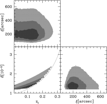
Figure 3: Constraints projected in the 2 parameter subspace from the 3 parameter space, assuming 6 lens candidates in sazhin05 are true lens events. From darker to lighter shaded regions, we show $68\%$, $95\%$, $99.7\%$ confidence limits. The dotted line in the $z_{l}$-$\delta$ plane indicates the limit of the prior given by Eq. (9).

We compute the number distribution of lenses with Eqs. (5) and (6). The lens candidates are identified in the medium deep images with limiting magnitude of $R\sim 24$, which correspond to $A=10{\rm arcmin^{-1}}$ and $z_{0}=0.78$ (the median galaxy redshift $\langle z\rangle=0.85$). From this, we compute the likelihood as

$${\mathcal{L}}=\frac{N^{x}\exp(-N)}{x!}\prod_{i=1}^{x}\left.\frac{dN}{d\theta}\right|_{\theta_{i}},$$ (8)

where $N=N(>1^{\prime\prime})$ is the total number of lenses with image separation larger than $1^{\prime\prime}$ (lenses with smaller image separations are quite hard to be identified) expected in the field, $x=6$ is the observed number of lenses, $\theta_{i}$ is the image separation of $i$-th lens. We compute likelihoods as a function of three parameters; the string redshift $z_{l}$, the dimensionless tension $\delta$, and the correlation length $\xi$, and derive constraints on these parameters. In doing so, we include the following prior

$$1.9^{\prime\prime}=9.2\times 10^{-6}<\delta\left.\frac{D_{ls}}{D_{os}}\right|_{z_{s}=0.46},$$ (9)

which originates from the fact that the redshift of CSL-1 is $z_{s}=0.46$.

The resulting constraints are shown in Fig. 3. The best-fit parameters are $z_{l}=0.13$, $\delta=1.4\times 10^{-5}$, and $\xi=180^{\prime\prime}$ (which corresponds to $0.3h^{-1}{\rm Mpc}$ at $z=0.13$). We find that we can place tight constraints on string parameters even from 6 lens events only: $z_{l}<0.22$ and $1.2<\delta/10^{-5}<1.8$ at $95\%$ confidence limit. Therefore we conclude that the statistics of lensing by a cosmic string are useful way to constrain properties of the cosmic string. Assuming the best-fit parameter set, we predict that the wide-field imaging of the field (see Sec. III for the specific setup) will be able to detect $\sim 270$ lens candidates with the image separations larger than $1^{\prime\prime}$.

V Conclusions

In this paper, we derived explicit expressions for the distributions of image separations of lensing by a cosmic string. We computed the number of nearby lensing events around one lensing event by a cosmic string. We considered both cases that the string is straight and fully wiggling in the field-of-view we are interested in.

It is quite hard to characterize a cosmic string from detailed investigation of a single lensing event, because of the degeneracy between parameters. We have found that the statistics of lensing events, i.e., comparing the theoretical number distribution of image separations with observations is an effective way to break the degeneracy and determine string parameters such as the string redshift and tension. We have shown that the detection of only several nearby lensing events is enough to place interesting new constraints on parameters. Our calculation indicates that a deep wide-field imaging in the field of string lens event will be able to find hundreds of additional lensing events, which offer valuable information on the cosmic string and hence the very early phase of our universe.

In this paper, we have assumed that the cosmic string is non-relativistic, i.e., we neglected the separation-angle correction from its velocity. Statistical study including the velocity effect would be challenging and necessary for the precise interpretation of the future observational data.

- (1) L. Pogosian, S. H. H. Tye, I. Wasserman and M. Wyman, Phys. Rev. D, 68, 023506 (2003).
- (2) L. Pogosian, M. Wyman and I. Wasserman, JCAP, 09, 008 (2004).
- (3) E. Jeong and G. F. Smoot, Astrophys. J., 624, 21 (2005).
- (4) A. S. Lo and E. L. Wright, astro-ph/0503120.
- (5) T. W. B. Kibble, astro-ph/0410073.
- (6) J. Polchinski, hep-th/0412244.
- (7) L. Perivolaropoulos, astro-ph/0501590.
- (8) N. T. Jones, H. Stoica and S.-H. H. Tye, Phys. Lett. B, 563, 6 (2003).
- (9) G. Dvali and A. Vilenkin, JCAP, 0403, 010 (2004).
- (10) E. J. Copeland, R. C. Myers and J. Polchinski, JHEP, 0406, 013 (2004).
- (11) M. G. Jackson, N. T. Jones and J. Polchinski, hep-th/0405229.
- (12) R. Jeannerot, J. Rocher and M. Sakellariadou, Phys. Rev. D 68, 103514 (2003).
- (13) M. Sazhin et al., Mon. Not. Roy. Astron. Soc., 343, 353 (2003); M. Sazhin et al., astro-ph/0506400.
- (14) M. Donaire and A. Rajantie, hep-ph/0508272.
- (15) D. Huterer and T. Vachaspati, Phys. Rev. D, 68, 041301 (2003).
- (16) B. Shlaer and S. -H. H. Tye, Phys. Rev. D, 72, 043532 (2005).
- (17) A. Vilenkin, Astrophys. J., 282, L51 (1984).
- (18) S. Miyazaki et al., Publ. Astron. Soc. Jap., 54, 833 (2002).
- (19) M. Sazhin et al., Astron. Lett., 31, 73 (2005).