Error Analysis for Dual-Beam Optical Linear Polarimetry

Abstract

In this paper we present an error analysis for polarimetric data obtained with dual-beam instruments. After recalling the basic concepts, we introduce the analytical expressions for the uncertainties of polarization degree and angle. These are then compared with the results of Monte-Carlo simulations, which are also used to briefly discuss the statistical bias. Then we approach the problem of background subtraction and the errors introduced by a non-perfect Wollaston prism, flat-fielding and retarder plate defects. We finally investigate the effects of instrumental polarization and we propose a simple test to detect and characterize it. The application of this method to real VLT-FORS1 data has shown the presence of a spurious polarization, which is of the order of $\sim$1.5% at the edges of the field of view. The cause of this effect has been identified with the presence of rather curved lenses in the collimator, combined with the non complete removal of reflections by the coatings. This problem is probably common to all focal-reducer instruments equipped with a polarimetric mode. An additional spurious and asymmetric polarization field, whose cause is still unclear, is visible in the $B$ band.

1. Introduction

Performing polarimetry basically means measuring flux differences along different electric field oscillation planes. In ground-based astronomy this becomes a particularly difficult task, due to the variable atmospheric conditions which make it difficult to detect the relatively low polarization degrees which characterize most astronomical sources (a few percent; see for example Leroy, 2000). These fluctuations, in fact, introduce flux variations among different polarization directions which can be eventually mistaken for genuine polarization effects.

This problem has been solved in a number of different ways reviewed by Tinbergen (1996) and to which we refer the reader for a detailed description. In this paper we will focus on the so-called dual-beam configuration, which is the most popular one for instruments currently mounted at large telescopes. Despite new technologies, the basic concept of astronomical dual-beam polarimeters (see for example Appenzeller, 1967; Scarrot et al., 1983) has remained unchanged. A mask placed on the focal plane, which prevents image (or spectra) overlap, is followed by a Wollaston prism, which splits the incoming beam into two rays characterized by orthogonal polarization states and separated by a suitable angular throw. The rotation of polarization plane is usually achieved with the introduction of a turnable retarder plate (half or quarter wave for linear and circular polarization, respectively) just before the Wollaston prism (see for example Schmidt, Stockman & Smith, 1992). Recently new solutions have been proposed, in order to fully solve the problem in one single exposure (see Oliva 1997 and Pernechele et al. 2003 for an example application), but so far they have been implemented in a few cases only.

Alternatives to Wollaston-based systems have been devised. They are mainly based on the charge transfer in CCDs, which allows an on-chip storage of two different polarization states, which are obtained rotating a polarization modulator. After the pioneering work of McLean, Aspin & Reitsema (1983), this technique, originally proposed by P. Stockman, has been successfully applied in a number of instruments (McLean, 1997).

In this work we address the most relevant problems which are connected to two-beam polarimetric observations and data reduction. The paper is organized as follows. In Sec. 2 we introduce the basic concepts of the problem and in Sec. 3 we recall the analytical expressions for the uncertainties of polarization degree and angle, which are then compared to Monte-Carlo simulations in Sec. 4. In the same section we also recap the basics of polarization bias. Sec. 5 deals with the effects of background on the polarization measurements and Sec. 6 treats the flat-fielding issues. Sec. 7 is devoted to the deviations of the Wollaston prism from the ideal behaviour, the consequences of retarder plate defects are addressed in Sec. 8 while the effects of post-analyzer optics are discussed in Sec. 9. Sec. 10 is dedicated to the instrumental polarization and Sec. 11 deals with the case of VLT-FORS1. Finally, in Sec. 12 we discuss and summarize our results.

2. Basic Concepts

The polarization state of the incoming light can be described through a Stokes vector $\vec{S}(I,Q,U,V)$ (see, for example, Chandrasekhar, 1950). Its components, also known as Stokes parameters, have the following meaning: $I$ is the intensity, $Q$ and $U$ describe the linear polarization and $V$ is the circular polarization. Linear polarization degree $P$ and polarization angle $\chi$ are related to the Stokes parameters as follows:

$$P=\frac{\sqrt{Q^{2}+U^{2}}}{I}\equiv\sqrt{\bar{Q}^{2}+\bar{U}^{2}}$$ (1)

$$\chi=\frac{1}{2}\arctan\frac{U}{Q}$$ (2)

where we have introduced the normalized Stokes parameters $\bar{Q}=Q/I$ and $\bar{U}=U/I$. The above relations can be easily inverted to yield:

$$\bar{Q}=P\;\cos 2\chi\;\;;\;\;\bar{U}=P\;\sin 2\chi$$ (3)

Finally, the circular polarization degree, not discussed in this paper, is simply $P_{c}=\bar{V}\equiv V/I$. For the sake of clarity, we will set $V$=0 and neglect all circular polarization effects throughout the paper.

The ideal measurement system for linear polarization is composed of a half-wave retarder plate (HWP) followed by the analyzer, which is a Wollaston prism (WP) producing two beams with orthogonal polarization directions. In general, each of these elements can be treated as a mathematical operator that acts on the input Stokes vector $\vec{S}$ (see for example Shurcliff, 1962; Goldstein, 2003). What one measures on the detector is the intensities in the ordinary and extraordinary beams at a given $HWP$ angle $\theta_{i}$, which are related to the Stokes parameters by:

$$\left\{\begin{array}[]{ccc}f_{O,i}&=&\frac{1}{2}\left[I+Q\;\cos 4\theta_{i}+U\;\sin 4\theta_{i}\right]\\ &&\\ f_{E,i}&=&\frac{1}{2}\left[I-Q\;\cos 4\theta_{i}-U\;\sin 4\theta_{i}\right]\end{array}\right.$$ (4)

If the observations are carried out using $N$ positions for the HWP, the whole problem of computing $I,Q$ and $U$ reduces to the solution of the 2$N$ linear equations system given by Eqs. 4. It is clear that, having three unknowns ($I,Q$ and $U$), at least $N$=2 HWP position angles have to be used.

Introducing the normalized flux differences $F_{i}$

$$F_{i}\equiv\frac{f_{O,i}-f_{E,i}}{f_{O,i}+f_{E,i}}$$ (5)

and noting that $f_{O,i}+f_{E,i}=I$, Eqs. 4 reduce to the following $N$ equations:

$$F_{i}=\bar{Q}\cos 4\theta_{i}+\bar{U}\sin 4\theta_{i}=P\;\cos(4\theta_{i}-2\chi)$$ (6)

We note that each $F$ parameter is totally determined by a single observation, and it is therefore independent from sky conditions changes. It is also worth mentioning that alternative approaches to the normalized flux ratios exist. One example can be found in Miller, Robinson & Goodrich (1987).

In principle, one can use any set of HWP angles to solve the problem, but is is easy to show that adopting a constant step $\Delta\theta$=$\pi/8$ is the optimal choice. In fact, besides minimizing the errors of the Stokes parameters, this choice makes the solution of Eqs. 6 trivial:

$$\bar{Q}=\frac{2}{N}\;\sum_{i=0}^{N-1}F_{i}\cos(\frac{\pi}{2}i)$$ (7)

$$\bar{U}=\frac{2}{N}\;\sum_{i=0}^{N-1}F_{i}\sin(\frac{\pi}{2}i)$$ (8)

Finally, it prevents the “power leakage” (see, for instance, Press et al., 1999) when one is to perform a Fourier analysis (see below).

In the ideal case, the normalized flux differences $F_{i}$ obey Eq. 6, which is a pure cosinusoid. Since all possible effects introduced by the HWP must reproduce after a full revolution, it is natural to consider them as harmonics of a fundamental function, whose period is $2\pi$.

Therefore, if $\theta_{i}=\pi i/8$, Eq. 6 can be rewritten as the following Fourier series:

$$F_{i}=a_{0}+\;\sum_{i=1}^{N/2}a_{k}\;\sin(k\frac{2\pi i}{N})+b_{k}\;\cos(k\frac{2\pi i}{N})$$

where the Fourier coefficients are given by

$$a_{0} = \frac{1}{N}\sum_{i=0}^{N-1}F_{i}$$

$$a_{k} = \frac{2}{N}\;\sum_{i=0}^{N-1}F_{i}\;\cos(k\frac{2\pi i}{N})$$ (9)

$$b_{k} = \frac{2}{N}\;\sum_{i=0}^{N-1}F_{i}\;\sin(k\frac{2\pi i}{N})$$

which are valid for $N=4,8,12,16$. Comparing Eqs. 2 with Eq. 6, it is clear that the polarization signal is carried by the $k=N/4$ harmonic. In a quasi-ideal case, all Fourier coefficients are expected to be small compared with $a_{N/4}$ and $b_{N/4}$ and deviations from this behaviour could arise from a number of effects. For such an approach to the error analysis and for the meaning of the various harmonics, the reader is referred to Fendt et al. (1996). Here we just notice that the $a_{0}$ term, which should be rigorously null in the ideal case, is related to the deviations of the WP from the ideal behaviour (see Sec. 7).

In general, a Fourier analysis is meaningful when $N$=16, and can reveal possible problems directly related to the HWP quality (cf. Sec. 8). In most cases, though, due to practical reasons, one typically uses $N$=4 and, in that circumstance, a different error treatment is required.

3. Analytical Error analysis

Under the assumption that all relevant quantities are distributed according to Gaussian laws, one can analytically derive simple expressions for the corresponding errors of the final results. As we will see in the next section, this assumption is not always correct and, when this happens, a numerical treatment is required in order to test the analytical results and their range of validity. Assuming that the background level is the same in the ordinary and extraordinary beams and that the read out noise can be neglected, the analytical expression for the absolute error of $P$ can be readily derived (see for example Miller, Robinson & Goodrich, 1987) propagating the various errors through the relevant equations:

$$\sigma_{P}=\frac{1}{\sqrt{N/2}\;SNR}$$ (10)

where $SNR$ is the signal-to-noise ratio of the intensity image ($f_{O}+f_{E}$). The signal-to-noise one expects to achieve in the polarization degree, $SNR_{P}=P/\sigma_{P}$, is simply given by:

$$SNR_{P}=\sqrt{\frac{N}{2}}\;P\;SNR$$

As for the error of $\chi$, this is given by:

$$\sigma_{\chi}=\frac{1}{2\sqrt{N/2}\;P\;SNR}\equiv\frac{\sigma_{P}}{2P}$$ (11)

from which it is clear that, at variance with the polarization degree, the accuracy of the polarization angle does depend on the intrinsic polarization degree.

4. Monte Carlo simulations

The analytical treatment presented in Sec. 3 relies on the assumption that all relevant variables obey Gaussian statistics. Numerical simulations are required in order to derive more realistic distributions and to verify the validity of the analytical results. One can easily implement the concepts we have developed until now in a Monte Carlo (MC) code, which also allows higher sophistication, like the inclusion of Poissonian noise. With this tool one can readily investigate the effects of non-Gaussian distributions of the derived quantities, the most important of which is the systematic error of the polarization, as it was first pointed out by Serkowski (1958).

4.1. Linear Polarization Bias

Due to the various noise sources, the vector components $\bar{Q}$ and $\bar{U}$ are Normally distributed, but since $P$ is defined as the quadrature sum of $\bar{Q}$ and $\bar{U}$, the statistical errors always add in the positive direction, leading to a systematic increase of the estimated polarization degree, thus introducing a bias. The problem was addressed by several authors, both with analytical and numerical methods (Serkowski, 1958; Wardle & Kronberg, 1974; Simmons & Stewart, 1985; Clarke & Stewart, 1986; Sparks & Axon, 1999). We refer the reader to those papers for a detailed description of the problem, while here we just recall the basic concepts and we apply them to our case.

The polarization bias is usually quantified using a robust estimator, supposedly giving a statistically significant representation of the observed value, which is then compared with the input polarization in order to derive the systematic correction. Different choices have been adopted (see Sparks & Axon, 1999). Following the considerations by Wardle & Kronberg (1974) we have here adopted the mode $\langle P\rangle$ of the distribution in order to estimate the bias, that we therefore define as $\Delta P=\langle P\rangle\/-P_{0}$, where $P_{0}$ is the input polarization. Once applied to to the observed data, the bias correction $\Delta P$ tends to restore the symmetry of the deviation distribution (see for example Sparks & Axon, 1999, their Fig. 4).

In Fig. 1 we show the results of our MC simulations for the estimated RMS error of the polarization $\sigma_{P}$ (upper panel) and polarization bias $\Delta P$ (lower panel) for $N$=4. Following Sparks & Axon (1999), we have used $\eta\equiv P_{0}\cdot SNR$ and $\langle\eta\rangle\equiv\langle P\rangle\cdot SNR$ as independent variables in our plots. As we had anticipated, $\sigma_{P}$ follows the analytical prediction of Eq. 10 when $\eta>$2. For lower values of $\eta$, $\sigma_{P}$ tends to be systematically smaller than the analytical prediction and it converges to the value expected for the Rayleigh distribution (dashed line),which becomes a very good approximation for $\eta<$0.5, provided that $SNR>$3. For intermediate values of $\eta$, the distribution is described by a Rice function (Rice, 1944). In conclusion, one can safely use the analytical solution given by Eq. 10 for $\eta\geq$2 only.

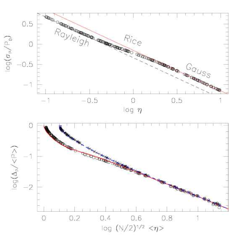
Figure 1.— Upper panel: comparison between the RMS error on the polarization degree from MC simulations (circles) and Eq. 10. The dashed line traces the expected RMS error for the Rayleigh distribution (see text). Lower panel: bias estimated using the mode (circles) and the average (crosses). For comparison, the solid curve traces the Wardle & Kronberg (1974) solution for the mode, while the dashed line is the Sparks & Axon (1999) solution for the average.

As for the polarization bias, we have plotted it as a function of measurable quantities, namely the signal-to-noise and the observed polarization $\langle P\rangle$.

The results of our MC simulations, as plotted in the lower panel of Fig. 1, are in good agreement with the analytical solution found by Wardle & Kronberg (1974) for the same statistical estimator. For comparison, we have also plotted the results one obtains when the average is adopted (crosses). For $\sqrt{N/2}\;\langle\eta\rangle>$4 the relation between $\log(\Delta P/\langle P\rangle\/)$ and $\log(\sqrt{N/2}\;\langle\eta\rangle)$ is well approximated by a linear law. A least squares fit gives the following result:

$$P_{0}=\langle P\rangle\/\left[1-\left(\frac{0.62}{\sqrt{N/2}\;\langle\eta\rangle}\right)^{1.92}\right]$$

which can be used to correct the observed polarization values according to the input signal-to-noise ratio, measured polarization and number of HWP positions. In general, the bias effect is present even at reasonably high values of $SNR$ when the polarization is small and $\sigma_{P}$ and $\Delta P$ tend to become similar, so that the systematic bias correction is comparable to the random uncertainty of the polarization. This is better seen in Fig. 2, where we have plotted the ratio $\Delta P$ over $\sigma_{P}$ as a function of $P_{0}/\sigma_{P}\equiv SNR_{P}$ deduced from our simulations. As anticipated, for low values of $SNR_{P}$, the ratio between $\Delta P$ and $\sigma_{P}$ tends to unity, with some variations among different estimators. For $SNR_{P}\geq$3 the bias correction is less than 10% of the expected accuracy, and it is, therefore, negligible. Moreover, above that threshold, all estimators give practically identical results.

In Fig. 2 we have plotted, for comparison, the function computed by Simmons & Stewart (1985), who have used a Maximum Likelihood estimator in order to evaluate the bias. As these authors have shown, this is the best estimator for $SNR_{P}\leq$0.7, while for $SNR_{P}>$0.7 the mode, first used by Wardle & Kronberg (1974), should be used.

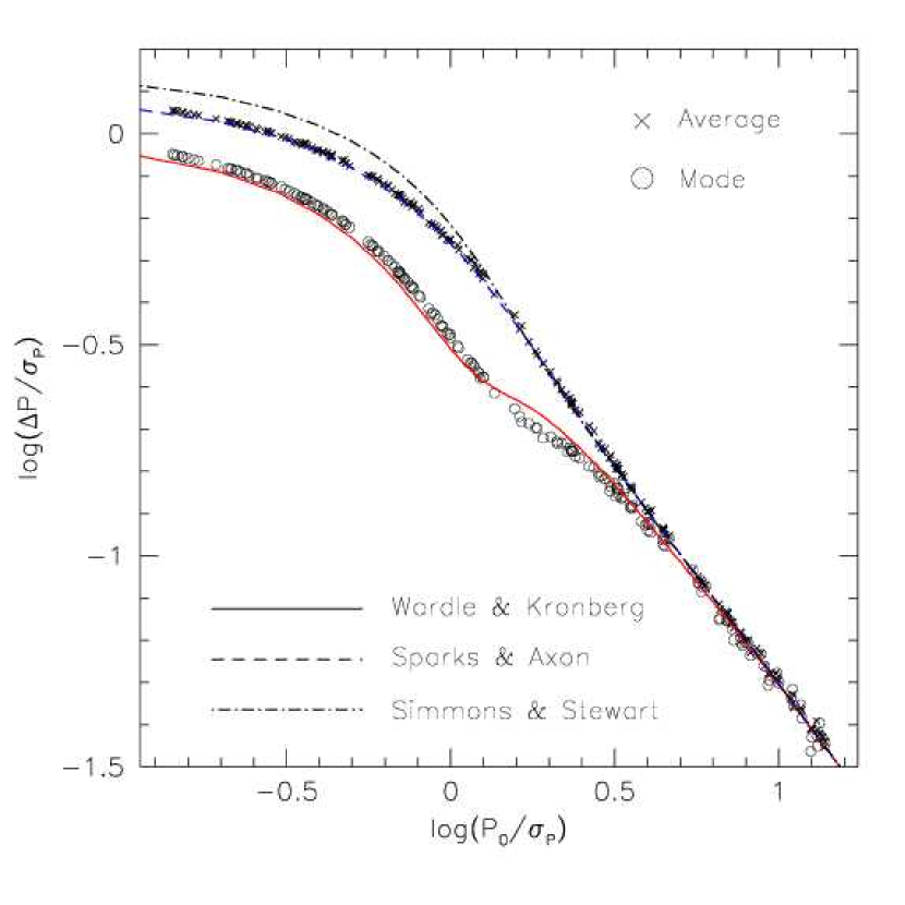
Figure 2.— Comparison between systematic bias $\Delta P$ and random error $\sigma_{P}$ for different estimators as a function of input polarization signal-to-noise ratio.

5. The Effects of the Background

Until now we have assumed that one is able to perfectly subtract the background contribution. This is most likely the case when one is to perform polarimetric measurements on point-like sources, since in that situation local background subtraction is in most cases straightforward.

We remark that the background, whatever its nature is, must be subtracted before the calculation of normalized Stokes parameters (see also Tinbergen, 1996), so that possible background polarization is vectorially removed.

If we assume that the object is characterized by $P_{o}$ and $\chi_{o}$ and the background by $P_{b}$ and $\chi_{b}$, the two polarization fields can be expressed using the Stokes vectors defined as $\vec{S_{o}}(I_{o},I_{o}P_{o}\cos 2\chi_{o},I_{o}P_{o}\sin 2\chi_{o})$ and $\vec{S_{b}}(I_{b},I_{b}P_{b}\cos 2\chi_{b},I_{b}P_{b}\sin 2\chi_{b})$, where we have neglected any circular polarization. Since Stokes vectors are additive (see for example Chandrasekhar, 1950), the resulting polarization field is described by $\vec{S}=\vec{S_{o}}+\vec{S_{b}}$ and, therefore, the total polarization is given by the following formula:

$$P=\frac{I_{o}P_{o}}{I_{o}+I_{b}}\sqrt{1+r^{2}+2r\cos[2(\chi_{o}-\chi_{b})]}$$

where $r=(I_{b}P_{b})/(I_{o}P_{o})$, i.e. the ratio between the polarized fluxes of background and object. The corresponding polarization angle is

$$\chi=\frac{1}{2}\arctan{\frac{\sin 2\chi_{o}+r\;\sin 2\chi_{b}}{\cos 2\chi_{o}+r\;cos2\chi_{b}}}$$

Clearly, the background is going to influence significantly the object when $r\gtrsim 1$. For $r\sim 1$ one can write:

$$P\simeq\frac{P_{o}}{\sqrt{2}}\sqrt{1+\cos[2(\chi_{o}-\chi_{b})]}$$

which implies that, for comparable polarized fluxes, the resulting polarization is nulled when the polarization fields are perpendicular ($|\chi_{o}-\chi_{b}|=\pi/2$).

6. Flat fielding

One of the basic problems one has to face when reducing the data produced by dual-beam instruments is the flat-fielding. Due to the fact that image splitting occurs after the focal mask, the collimator and the HWP, one would in principle need to obtain flat exposures with all optical components in the light path. Unfortunately, in all practical conditions, this introduces strong artificial effects due to the strong polarization typical of flat-field sources (either twilight sky or internal screens). In principle one can reduce this effect using the continuous rotation of the HWP as a depolarizer. This is implemented, for example, in EFOSC2, currently mounted at the ESO-3.6m telescope (Patat, 1999) and it is effective only if the HWP rotation time is much shorter than the required exposure time. The depolarizing effect can also be achieved by averaging flats taken the same set of HWP angles used for the scientific exposures. In fact, with the usage of the optimal angle set (see Sec. 2), one has that

$$\sum_{i=0}^{N-1}f_{O,i}=\frac{N}{2}I$$

and a similar expression for $f_{E,i}$, which do not contain any polarization information. The problem is that this is true only if the source is stable in intensity, which is surely not the case for the twilight sky and probably not really true for most lamps.

An alternative solution (at least for imaging) is the usage of a set of twilight flats obtained without HWP and WP. If on the one hand this eliminates source polarization, on the other hand it does not allow for a proper flat field correction. In fact, while the pixel-to-pixel variations are properly taken into account, the large scale patterns are not, due to the beam split that maps a given focal plane area into two distinct regions of the post-WP optics and detector. Moreover, these calibrations do not carry any information about possible spatial effects introduced by the HWP and the WP. However, as the simulations show, this problem becomes milder if some redundancy is introduced. For example, if one uses $N$=4 HWP positions, the ordinary and extraordinary ray will just swap when the angle differs by $\pi/4$ within each of the two redundant pairs ($f^{i}_{O}=-f^{i+2}_{E}$, see Eqs. 4). This tends to cancel out the flat-field effect and becomes more efficient if the maximum redundancy ($N$=16) is used. It must be noticed, however, that time dependent effects, like fringing, may affect the redundant pairs in a different way, therefore decreasing the cancellation efficiency.

7. Effects of a non-ideal Wollaston prism

So far we have assumed that our system is described by Eqs. 4, i.e. that the Wollaston prism splits incoming unpolarized light into identical fractions. A deviation from this ideal behaviour can be described by the introduction of a new parameter $t$ in Eqs. 4, which can be reformulated as follows:

$$\left\{\begin{array}[]{ccl}f_{O,i}&=&t\left[I+Q\;\cos 4\theta_{i}+U\;\sin 4\theta_{i}\right]\\ &&\\ f_{E,i}&=&(1-t)\left[I-Q\;\cos 4\theta_{i}-U\;\sin 4\theta_{i}\right]\end{array}\right.$$ (12)

An ideal system is obtained for $t=\frac{1}{2}$. Now, for unpolarized light ($Q$=$U$=0), these new equations give $f_{O,i}=tI$ and $f_{E,i}=(1-t)I$ for all HWP angles, so that all normalized flux differences turn out to be identical, i.e. $F_{i}=2t-1$. Therefore, the value of $t$ can be directly estimated observing an unpolarized source.

In the simplest situation, where $N$=2, neglecting the presence of the $t$ term would lead to a spurious polarization degree $P=\sqrt{2}\;(2t-1)$, with a polarization angle $\chi=\pi/8$. It is interesting to note that this is not the case, for example, when $N$=4. In that situation, in fact, because all redundant $F$’s are identical, Eqs. 7 and 8 would correctly yield null Stokes parameters.

The problem when the incoming light is polarized is more complicated, since the normalized flux differences are not anymore a linear combination of $\bar{Q}$ and $\bar{U}$, as one can verify from Eqs. 12:

$$F_{i}=\frac{\kappa+\bar{Q}\cos 4\theta_{i}+\bar{U}\sin 4\theta_{i}}{1+\kappa\bar{Q}\cos 4\theta_{i}+\kappa\bar{U}\sin 4\theta_{i}}$$ (13)

where we have set $\kappa=2t-1$ ($|\kappa|\leq$1, $\kappa$=0 in the ideal case). If $\kappa$ is known, one can correct the observed $f_{O}$ and $f_{E}$ dividing them by $2t$ and $2(1-t)$ respectively before following the procedure adopted for the ideal case. Of course, if the source has a known polarization (e.g. a polarized standard), one can use this information together with the observed $F$ ratios to derive $\kappa$ for each HWP angle, according to the following relation:

$$\kappa_{i}=\frac{\bar{Q}\cos 4\theta_{i}+\bar{U}\sin 4\theta_{i}-F_{i}}{F_{i}\;(\bar{Q}\cos 4\theta_{i}+\bar{U}\sin 4\theta_{i})}$$

If the input polarization is unknown, then one can in principle derive $\kappa$ from the observations themselves, provided that $N\geq$4. In fact, after introducing the parameter

$$g_{j}=\frac{1+F_{j-1}\;F_{j+1}}{F_{j-1}+F_{j+1}}$$ (14)

and using Eqs. 13, it is easy to demonstrate that

$$\kappa_{j}=g_{j}\pm\sqrt{g^{2}_{j}-1}$$ (15)

where $j=1,...,N/2-2$ and the positive sign refers to the case $g_{j}\leq 0$. For instance, for $N=4$, one can determine two independent estimates of $\kappa$, which can be averaged to improve on the accuracy.

It is interesting to note that, when $P\ll 1$, Eq. 13 can be approximated as $F_{i}\simeq\kappa+\bar{Q}\cos 4\theta_{i}+\bar{U}\sin 4\theta_{i}$. If $N$ is a multiple of 4 (i.e. if the $F$ function is sampled for an integer number of periods $\pi/2$), one has that

$$\kappa\approx\frac{1}{N}\;\sum_{i=0}^{N-1}F_{i}\equiv a_{0}$$ (16)

which clarifies the meaning of the $a_{0}$ term in the Fourier series (see Eq. 2).

It is worth mentioning that the redundancy on the $F$ parameters does eliminate the effects of a non ideal WP to a large extent. For example, a blind application of Eqs. 7 and 8 to the case of $N$=4 gives the following result:

$$\frac{2}{N}\;\sum_{i=1}^{N-1}F_{i}\cos(4\theta_{i})=\bar{Q}\;\frac{1-\kappa^{2}}{1-\kappa^{2}\bar{Q}^{2}}$$

and a similar expression for $\bar{U}$. If the polarization is small ($P_{0}\leq 0.1$), we have that $\kappa^{2}\bar{Q}^{2}\ll 1$ and therefore the application of the ideal case procedure to a non ideal situation would lead to a value of $\bar{Q}$ which is $(1-\kappa^{2})$ times smaller than the real one. Since the same is true for $\bar{U}$, the resulting polarization $P$ will also be $(1-\kappa^{2})$ times smaller than the input value, while the polarization angle remains unchanged. For example, if $|\kappa|\leq 0.2$, $\sigma_{P}/P$ is less than 4%.

Eqs. 12 describe a particular case only, where the incoming unpolarized flux is distributed into two fractions $t$ and $(1-t)$. More in general, one should replace the term $(1-t)$ with an independent parameter $s$, so that the fraction of light split by the WP in the ordinary and extraordinary ray become uncorrelated. Using the same procedure, it is easy to demonstrate that one can estimate the ratio $\kappa_{j}=(t-s)/(t+s)$ still using Eq. 15.

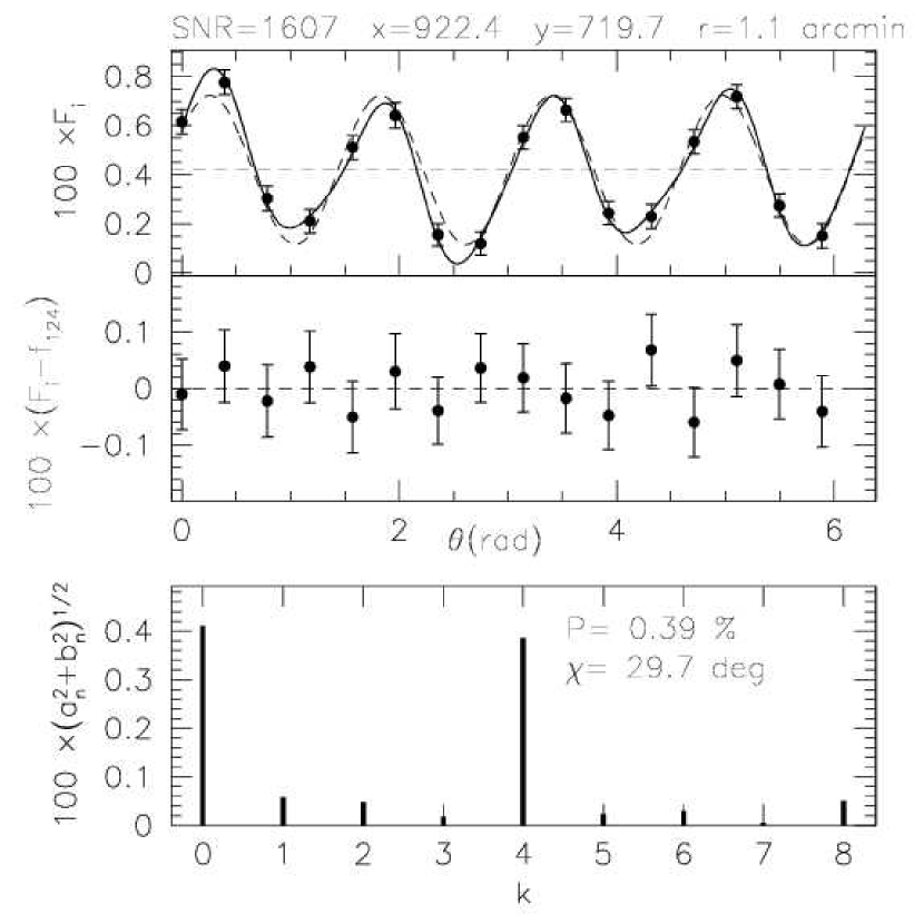
Figure 3.— Example of Fourier Analysis applied to archival VLT-FORS1 observations of a bright star in the $V$ passband (see text). Upper panel: normalized flux differences. Partial reconstructions using 8 harmonics (solid curve) and the 4-th harmonic only (dashed curve) are traced. The dashed horizontal line is placed at the average of $F$ values ($a_{0}$). Central panel: residuals after subtracting the $k$=1,2,4 components. Lower panel: harmonics power spectrum.

Another effect we have investigated is the possibility that the difference in polarization direction between the ordinary and the extraordinary ray of the WP is not $\pi/2$. If we call $\Delta\alpha$ the deviation from this ideal angle, using the general expression of the Mueller matrix for a linear polarizer (see for example Goldstein, 2003) and deriving the expressions for the normalized flux ratios, one gets:

$$F_{i}\simeq\frac{\bar{Q}}{2}[\cos(4\theta_{i}-2\Delta\alpha)+\cos 4\theta_{i}]+\frac{\bar{U}}{2}[\sin(4\theta_{i}-2\Delta\alpha)+\sin 4\theta_{i}]$$

where the approximation is valid under the assumption that $P\ll 1$. With the aid of this expression it is easy to conclude that for reasonably small values of $\Delta\alpha$ ($\leq$10^∘), the implied errors are of the order of 0.05% on the polarization degree and 5^∘ on the polarization angle, irrespective of the number of HWP positions used.

8. HWP defects

In the ideal case, the normalized flux differences are modulated by the HWP rotation according to Eq. 6, which is a pure cosinusoid. If defects are present on the HWP, like dirt or inhomogeneously distributed dust, one can expect spurious flux modulations, which are not related to the polarization of the incoming light and can reduce the performance of the instrument. As a consequence, error estimates based on pure photon statistics are systematically smaller than the actual ones.

These kinds of problems can be investigated with the aid of Fourier Analysis, following the procedure we have outlined at the end of Sec. 2. This method becomes particularly effective when the observations are taken sampling the full HWP angle range, i.e. 2$\pi$ which, given the choice of the optimal angle set $\theta_{i}$=$\pi i/8$, implies $N$=16 retarder plate positions. In these circumstances, one is able to determine the Fourier coefficients $a_{k}$ and $b_{k}$ for the first 8 harmonics, the fundamental ($k=1$) being related to local transparency fluctuations which repeat themselves after a full revolution, like dirt or dust. By definition (cf. Eq. 6), the fourth harmonic is directly related to the linear polarization, i.e. $a_{4}\equiv\bar{Q}$ and $b_{4}\equiv\bar{U}$. All other harmonics, with the only remarkable exception of the second one ($k$=2), are simply overtones of harmonics with lower frequencies and include part of the noise generated by the photon statistics, which is present at all frequencies and is therefore indicated as white noise. For this reason, the global random error is often estimated as the signal carried by the harmonics having $k$=3,5-8 (see for example Fendt et al., 1996, their Appendix A.3).

The second harmonic deserves a separate discussion. Ideally, the HWP operates as a pure rotator of the input Stokes vector, with the advantage that one does not need to rotate the whole instrument in order to analyze different polarization planes. In the real case, being the HWP usually constructed using bi-refringent materials, it is affected by the so-called pleochroism. This is a wavelength dependent variation of the transmission that takes place when the direction of the incoming light is changed with respect to the crystal lattice. Due to the way the HWP is manufactured, the crystals have an axial symmetry, which gives a period of $\pi$. Therefore, this effect is seen as the $k$=2 component.

In Fig. 3 we show a real case, where we have applied this analysis to archival data obtained with the FOcal Reducer/low dispersion Spectrograph (hereafter FORS1), which is currently mounted at the Cassegrain focus of ESO-VLT 8.2m telescope (Szeifert, 2002).

A bright (and supposedly unpolarized) star was observed using $N$=16 HWP positions. First of all, the Fourier Analysis indicates the presence of a small deviation of the WP from the ideal behaviour ($\kappa\approx a_{0}\simeq$4.1$\times$10^-3, see Sec. 7). Then, a clear polarization is detected, at the level of about 0.4% while all other components are smaller than 0.05% (this polarization is actually an instrumental effect present in FORS1. See Sec. 10). The effective significance of harmonics other than $k$=4 can be judged on the basis of the expected errors of the Fourier coefficients. For example, using the expression of $a_{k}$ one finds that

$$\sigma_{a_{k}}=\frac{2}{N\;SNR}\;\sqrt{\sum^{N}_{i=1}\cos^{2}k\frac{2\pi i}{N}}$$

With this kind of analysis, one can see that in the example of Fig. 3, $a_{k}$ and $b_{k}$ are consistent with a null value for $k$=3,5-7 (see the central panel). As for the $k$=1,2 harmonics, the Fourier coefficients are non null at a 2$\sigma$ level. Since for the test star it was $SNR\sim$1600, it is clear that to detect $k$=1,2 harmonics of this amplitude (0.05%), a $SNR\geq$3000 is required.

It is important to notice that the presence of these non-null harmonics is implicitly corrected for when one has a sufficient number of HWP positions covering the maximum period 2$\pi$. In the most common case, where $N$=4 angles spaced by $\pi$/8 are used, one can derive the fundamental (i.e. linear polarization, period $\pi$/2) and the first overtone (period $\pi$/4) only. The latter corresponds to the $k$=8 component of the $N$=16 cases, which therefore carries the high frequency information only. As a consequence, if other harmonics are present, they are not properly removed and contribute to the final error, practically setting the maximum accuracy one can achieve, irrespective of the SNR. Numerical simulations performed assuming a virtually infinite SNR show that in the presence of $k=1$ and $k=2$ components, the usage of $N$=4 HWP angles leads to systematic errors which are of the same order of the amplitude of the two harmonics. From this and the example reported in Fig. 3, one can estimate that the absolute maximum accuracy reachable with FORS1 using $N$=4 is of the order of 0.05%.

Another typical problem which affects the retarder plates is the chromatic dependence of the angle zero point. This is usually measured by means of a Glan-Thompson prism and it can change by more than 5^∘ across the optical wavelength range. The computed polarization angle can be corrected simply adding the HWP angle offset for the relevant wavelength (or effective wavelength in the case of broad band imaging). See, for example, Szeifert (2002).

Finally, we have investigated the effects produced by a deviation $\Delta\beta$ from the nominal phase retardance of an HWP ($\pi$). Using the general expression of the Mueller matrix for a retarder (see for example Goldstein, 2003), the normalized flux ratios turn out to be

$$F_{i} = \bar{Q}[\cos 4\theta_{i}-\sin^{2}2\theta_{i}(1-\cos\Delta\beta)]+$$

$$+ \frac{1}{2}\bar{U}\sin 4\theta_{i}\;(1+\cos\Delta\beta)+\bar{V}\sin 2\theta_{i}\sin\Delta\beta$$

from which it is clear that the measured linear polarization depends on the circular polarization of the input signal. For $V$=0 and $\Delta\beta\leq$10^∘ the corresponding absolute error of the polarization degree is less than 0.05%, while the outcome on the polarization angle is negligible. For $V\neq$0 the exact effect depends on the ratio between circular and linear polarization degrees. For example, for $\Delta=$10^∘ and $Q=U=V=$0.01, the absolute error of the computed polarization degree is about 0.1% for $N$=4, which decreases to 0.01% for $N$=16. It is worthwhile noting that this defect would be detected by a Fourier analysis as a component with a period $\pi$ and whose intensity is $|\bar{V}\sin\Delta|$.

9. Effects of post-analyzer optics

Typically the analyzer is followed by additional optics, like filters, grisms and camera lenses which, due to their possible tilt with respect to the optical axis, may behave as poor linear polarizers. In the most probable case where the polarization is produced by transmission (see also next section), the properties of post-analyzer (PA) components can be described by the following approximate Mueller matrix:

$$M_{PA}\simeq A\left(\begin{array}[]{ccccccc}1&&Bc&&Bs&&0\\ Bc&&1&&0&&0\\ Bs&&0&&C&&0\\ 0&&0&&0&&C\\ \end{array}\right)$$ (21)

where $A\approx$1, $C\approx$1, $c=\cos 2\varphi$, $s=\sin 2\varphi$ and $\varphi$ is the polarization angle (which can change across the field of view) while $B$ is related to the polarization degree introduced by the PA optics. This expression can be deduced from the general formulation (see Keller, 2002, Eq. 4.63) after applying the usual matrix rotation (see for example Keller, 2002, Eq. 2.5). If $\vec{S_{0}}=(I_{0},Q_{0},U_{0},V_{0})$ is the input Stokes vector, the effect of PA optics can be evaluated computing the Stokes vectors that correspond to the ordinary and extraordinary beams produced by the WP, transforming them using the operator $M_{PA}$ and using the resulting intensity components to compute the normalized flux differences $F_{i}$. After simple calculations, one arrives at the following expression:

$$F_{i}\simeq B\cos 2\varphi+\bar{Q_{0}}\cos 4\theta_{i}+\bar{U_{0}}\sin\theta_{i}$$

were we have assumed that $|B|\ll 1$, i.e. that the linear polarization induced by the PA optics is small. Given this expression, it is clear that the redundancy in the HWP positions ($N$=4, 8, 16) eliminates this problem, since the additive term $B\cos 2\varphi$ is not modulated by the HWP rotation, while for $N$=2 the derived polarization degree and angle would be affected, possibly in a severe way. If the optimal HWP angle set has been used, it is easy to verify that $B\cos 2\varphi=\sum_{i=0}^{N-1}F_{i}/N$, which is identical to Eq. 16. This means that, in a first approximation, it is not possible to disentangle between an imperfect WP and the presence of polarization in the PA optics. Therefore, the fact that $a_{0}\simeq$0.4% in Fig. 3, can actually be attributed to both kinds of problems. The PA optics effect becomes definitely stronger when these include highly tilted components, like the grisms. This is very well illustrated by the two examples of Fig. 4, where we show the results obtained using VLT-FORS1 archival data of a highly polarized star (Vela 1 95, $\alpha$=09:06:00, $\delta$=$-$47:19:00) and an unpolarized star (WD 1615-154, $\alpha$=16:17:55, $\delta$=$-$15:35:51), which were observed on the optical axis, where the instrumental polarization is known to be null (Szeifert, 2002).

In both cases the polarization degree deduced using $N$=2 (central panels) is markedly different from that derived with $N$=4 (upper panels) and the deviation is particularly severe for the unpolarized object. As one can finally notice, the resulting values of $B\cos 2\varphi$ show a strong wavelength dependency and are higher than 5% at about 800 nm. It is interesting to note that $B\cos 2\varphi\sim$0 at about 450 nm, i.e. at the wavelength where the anti-reflection coatings are optimized (see next section). This fact, together with the marked wavelength dependency and the much lower level seen in broad band imaging (see Fig. 3), strongly suggest that the effect seen in Fig. 4 is indeed produced by the tilted surfaces of the grism.

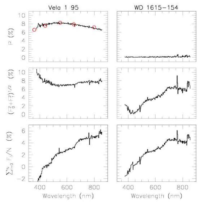
Figure 4.— VLT-FORS1 observations of Vela 1 95 (left panels) and WD 1615-154 (right panels). The plots show the linear polarization derived with $N$=4 HWP positions (upper panels), $N$=2 (middle panels) and $\sum_{i=0}^{N}F_{i}/N$ for $N$=4 (lower panels. See text for more details). The original spectra were obtained with the 300V grism and a slit of 1^′′; for presentation they have been binned to 25 Å. The empty circles in the upper left panel mark the broad-band polarimetric measurements for Vela 1 95 (UBVRI, from left to right).

10. Effects of instrumental polarization

So far, we have assumed that all optics preceding the analyzer do not introduce any polarization. Of course, this is not generally true (see for example Tinbergen, 1996, and Leroy 2000 for a general introduction to the subject).

To show the effect of instrumental polarization, we assume that the pre-analyzer optics, which include telescope mirrors, collimator, HWP and so on, introduce an artificial polarization, which depends on the position in the field. For the sake of simplicity, we assume these optics act as a non-perfect linear polarizer, characterized by a position dependent polarization degree $p(x,y)$ and polarization angle $\varphi(x,y)$. This can be described by the following Mueller matrix:

$$M_{I}(x,y)=\frac{1}{1+p}\left(\begin{array}[]{ccccc}1&&pc&&ps\\ pc&&1-ps^{2}&&psc\\ ps&&pcs&&1-pc^{2}\\ \end{array}\right)$$ (25)

where we have neglected circular polarization and we have set $s=\sin 2\varphi$ and $c=\cos 2\varphi$. For $p$=0 one obtains a totally transparent component, while $p$=1 gives an ideal linear polarizer.

If $\vec{S_{0}}(I_{0},Q_{0},U_{0})$ is the Stokes vector describing the input polarization state, it will be transformed by pre-analyzer optics into the vector $\vec{S_{1}}=M_{I}\cdot\vec{S_{0}}$ before entering the analyzer:

$$\begin{array}[]{llcl}I_{1}&(1+p)&=&I_{0}+pcQ_{0}+psU_{0}\\ Q_{1}&(1+p)&=&Q_{0}+pcI_{0}-ps^{2}Q_{0}+pcsU_{0}\\ U_{1}&(1+p)&=&U_{0}+psI_{0}+pcsQ_{0}-pc^{2}U_{0}\end{array}$$ (29)

and, therefore, the measurements would lead to $\vec{S_{1}}$ which would then need to be corrected for the instrumental effect inverting Eqs. 29, provided that $p(x,y)$ and $\varphi(x,y)$ are known.

Of course, if the observed source is known to be unpolarized, $p$ and $\varphi$ can be derived immediately, for example by placing a single target on different positions of the field of view or observing an unpolarized stellar field.

If the source is polarized, the problem becomes much more complicated, since Eqs. 29 are non linear in $c$ and $s$. The solution can be simplified assuming that $p\ll 1$ and $P_{0}\ll 1$, which is a reasonable hypothesis in most real cases, since instrumental polarization is typically less than a few percent. In these circumstances, Eqs. 29 can be rewritten as follows:

$$\begin{array}[]{lll}I_{1}&\simeq&I_{0}\\ Q_{1}&\simeq&Q_{0}+pI_{0}\;\cos 2\varphi\\ U_{1}&\simeq&U_{0}+pI_{0}\;\sin 2\varphi\end{array}$$ (33)

It is important to note that the instrumental polarization is not removed by the local background subtraction. Moreover, it is independent of the object’s intensity; in fact, using the previous expressions one can verify that

$$P=\sqrt{P_{0}^{2}+p^{2}+2P_{0}p\;\cos[2(\chi_{0}-\varphi)]}$$

where $P_{0}$ and $\chi_{0}$ are the input polarization degree and angle. From this expression it is clear that when $P_{0}\gg p$ it is also $P\approx P_{0}$, while in the case that object and instrumental polarization are comparable ($p\approx P_{0})$, the observed polarization is approximately given by

$$P\simeq\sqrt{2}P_{0}\sqrt{1+\cos[2(\chi_{0}-\varphi)]}$$

which, according to the value of $(\chi_{0}-\varphi)$, gives values that range from 0 to 2$P_{0}$. It is important to notice that the main difference between instrumental polarization and a polarized background is that the latter is effective only when $BGR\gtrsim I$ (see Sec. 5), while the former acts regardless of the object intensity and what counts is its polarization.

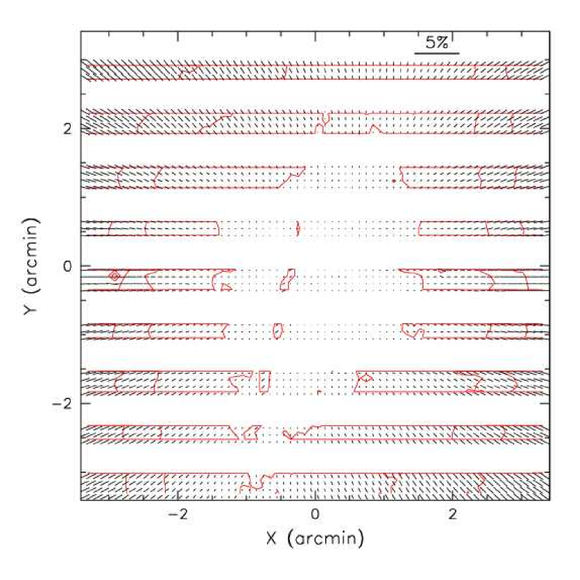
Figure 5.— FORS1 instrumental polarization map in the $B$ band. The contours trace 0.3%, 0.6% and 0.9% polarization levels. Coordinates, expressed in arcminutes, refer to the geometrical center of the detector.

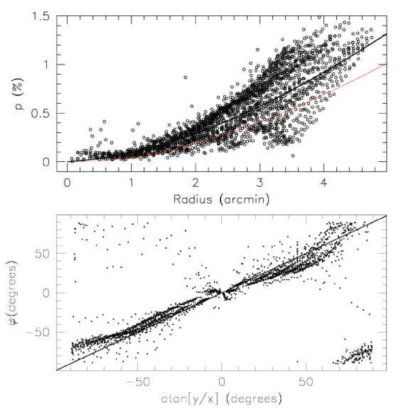
Figure 6.— Upper panel: FORS1 instrumental polarization radial profile for the $B$ band. Each point is the result of a 30$\times$30 px binning in the original images. Radius, expressed in arcminutes, is computed from the geometrical center of the detector. The thick line traces a linear least squares fit, while the thin line is the polarimetric ray-tracing prediction. Lower panel: instrumental polarization angle as a function of pixel polar angle. The solid line is not a fit to the data, but rather has unit slope and zero intercept.

With the aid of these approximate expressions (Eqs. 33), one can easily evaluate the instrumental polarization, provided that the input polarization field is known and the observed source covers a large fraction of the instrument field of view. In fact, solving Eqs. 33 for $\varphi$ and $p$ yields:

$$\tan 2\varphi\simeq\frac{U_{1}-U_{0}}{Q_{1}-Q_{0}}$$

and

$$p_{1}\simeq\frac{Q_{1}-Q_{0}}{I_{0}\cos 2\varphi}\;\;\;\;;\;\;\;\;p_{2}\simeq\frac{U_{1}-U_{0}}{I_{0}\sin 2\varphi}$$

where $p_{1}$ and $p_{2}$ are two independent estimates of $p$, that can be averaged to increase the accuracy.

As it is well known, the night sky shows a polarization which varies according to the ecliptic and galactic coordinates (see Leinert et al., 1998, for an extensive review). It is mostly dominated by the zodiacal light polarization, which reaches its minimum, below a few percent, at the anti solar position (Roach & Gordon, 1973). Since this is not expected to vary on the scales of a few arcminutes, in principle, relatively empty fields represent suitable targets for panoramic polarization tests, provided that the signal-to-noise ratio per spatial resolution element is of the order of several thousands.

11. The case of FORS1 at ESO-VLT

To show an example application, we have performed a test using real data obtained with FORS1 at the ESO-VLT. In this instrument, the polarimetric mode is achieved inserting in the beam a super-achromatic HWP and a WP, which has a throw of about 22^′′ (Szeifert, 2002).

We have identified in the ESO archive three sets of data obtained in rather empty fields in $B$, $V$ and $I$ passbands. Equatorial coordinates ($\alpha$, $\delta$), ecliptic longitude and latitude ($\lambda$, $\beta$), helio-ecliptic longitude ($\lambda-\lambda_{\odot}$), sky polarization degree and angle ($P_{sky}$, $\chi_{sky}$) are reported in Table 1 for the different fields. In all three cases the signal-to-noise ratio achieved on the sky background $I_{sky}$ in the combined images is larger than $SNR\simeq$200 per pixel. With such a signal and for a typical 1% polarization, the bias effect is expected to be small (see Fig. 1) and the RMS error of the polarization degree, according to Eq. 10, is of the order of 0.3%, while the uncertainty of $\chi$ is about 9^∘ (see Eq. 11). In order to further increase the accuracy and to allow for outlier rejection, we have computed a clipped average in 30$\times$30 px bins which, given the FORS1 detector scale (0^′′.2 px^-1), translates into an angular resolution of 6^′′.

Table 1 Data for the empty fields

Filter	$\alpha$	$\delta$	$\lambda$	$\beta$	$\lambda-\lambda_{\odot}$	$P_{sky}$	$\chi_{sky}$
	hh:mm:ss	dd:mm:ss	∘	∘	∘	%	∘
B	03:32:17	$-$27:44:24	$-$41.1	$-$45.1	128.1	6.45	+68.4
V	13:58:03	$-$31:22:21	218.6	$-$18.1	$-$159.7	1.74	$-$53.8
I	20:36:08	$-$13:06:39	308.0	+5.3	$-$110.0	1.34	+68.7

Since the instrumental polarization on the optical axis, measured with unpolarized standard stars, is smaller than 0.03% (Szeifert, 2002), one can be confident that the sky background polarization field ($P_{sky},\chi_{sky}$) measured close to that area is not affected by spurious effects (the values are reported in the last two columns of Table 1). Therefore, we can easily compute $p(x,y)$ and $\varphi(x,y)$ using the method previously outlined, where $I_{0}$=$I_{sky}$, $Q_{0}=I_{sky}P_{sky}\cos 2\chi_{sky}$ and $U_{0}=I_{sky}P_{sky}\sin 2\chi_{sky}$. The results of these calculations are presented in Figs. 5, 7 and 9. With the remarkable exception of the $B$ band, the instrumental polarization of FORS1 shows a quasi-symmetric radial pattern. For example, for the $V$ filter, the instrumental polarization remains below 0.1% within 1 arcmin from the geometrical center of the detector, while it grows up to $\sim$0.6% at 3 arcmin, to reach the maximum, i.e. $\sim$1.4%, at the corners of the field of view.

This is illustrated in the upper panels of Figs. 6, 8 and 10, where we have plotted the estimated instrumental polarization for each 30 $\times$ 30 px bin as a function of its average distance $r$ from the center. The deviation from a perfect central symmetry is distinctly shown by the dispersion of the points, which is larger than the measurement error. Particularly marked is the case of the $B$ band, which shows a strong azimuthal dependence and deserves a separate discussion (see next section). For the $V$ band there is a systematic deviation from central symmetry for a polar angle $\alpha=\arctan(y/x)$ between 10^∘ and 80^∘. This region is probably disturbed by the presence of a saturated star and a reflection caused by the HWP, visible in the input images. Excluding these points, a linear least squares fit to the $V$ data gives

$$p(r)=0.012r+0.046r^{2}+0.002r^{3}$$

where $r$ is expressed in arcminutes (Fig. 8, solid curve). The $I$ band shows the smoothest behaviour and the observations are described very well by the following polynomial:

$$p(r)=-0.017r+0.105r^{2}-0.006r^{3}$$

The absolute RMS deviations shown by the data from the best fits are of the order of 0.05%, so that in these two passbands the spurious polarization can be corrected with an accuracy which is comparable to that dictated by the photon statistics. In both cases, but especially in the $I$ band, the pattern is remarkably radial, as shown in the lower panels of Figs. 8 and 10, where we have plotted $\varphi$ as a function of polar angle $\alpha$.

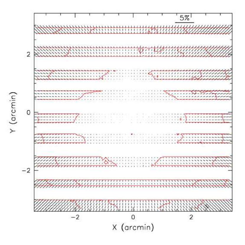
Figure 7.— Same as Fig. 5 for the $V$ band. The dark segment marked by a circle in the lower right corner indicates the values obtained from an unpolarized standard star.

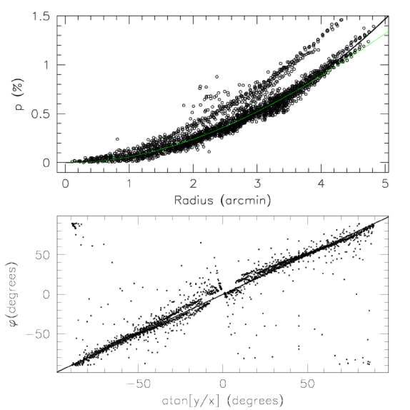
Figure 8.— Same as Fig. 6 for the $V$ band.

In order to verify these results for the $V$ filter, we have carried out a test observing an unpolarized standard star placed in the lower right corner of the detector. Measured polarization was $P$=0.92$\pm$0.04% and $\chi$=$-$48${}^{\circ}\pm$1^∘.4 while, according to the previous analysis, the expected instrumental polarization in that position is $p$=0.96% and $\varphi=-$51^∘.9, which are in very good agreement with each other (see also Fig. 7, lower right corner).

Once the instrumental polarization is mapped, one can correct for it using the approximate Eqs. 33, which hold when $p$ and $P_{0}$ are small and only if the instrumental polarization is produced by a linear polarizer preceding the analyzer.

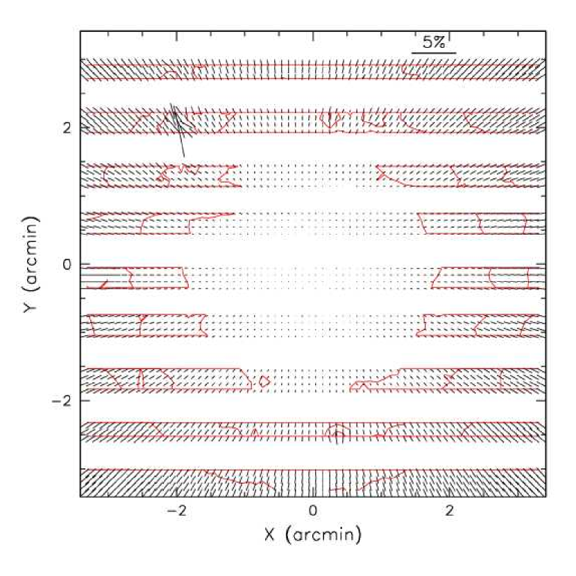
Figure 9.— Same as Fig. 5 for the $I$ band.

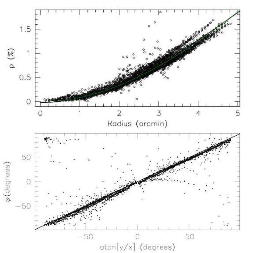
Figure 10.— Same as Fig. 6 for the $I$ band.

11.1. The cause of instrumental polarization in FORS1

As we have seen, the spurious polarization detected in FORS1 in $V$ and $I$ passbands has a clear central symmetry, it is null on the optical axis Szeifert (2002), shows a radial pattern and grows with the distance from the optical axis. All these facts suggest that this must be generated by the optics which precede the analyzer, i.e. within the collimator. In fact, when a light beam enters an optical interface along a non-normal direction, the component of the transmitted beam perpendicular to the plane of incidence is attenuated, according to Fresnel equations (see for example Born & Wolff, 1980). As a consequence, the emerging beam is linearly polarized in a direction which is parallel to the plane of incidence. If the surface is curved, as it is the case of lenses, the incidence angle quickly increases moving away from the optical axis and this, in turn, produces an increase in the induced polarization. The effect becomes more pronounced if the lens is strongly curved, i.e. if the curvature radius is comparable to its diameter. Of course, on the optical axis, the incidence angle is null, so that no polarization is produced. Therefore, at least from a qualitative point of view, the polarization induced by transmission has all the required features to explain the observed pattern.

The polarization induced by transmission can be easily evaluated using the appropriate expression for the corresponding Mueller matrix (see Keller, 2002, Eq. 4.63). For a typical refraction index $n$=1.5 and an incidence angle of 30^∘, refraction through an uncoated glass would produce a polarization of about $B$=1.7 % per optical surface. This polarization is usually reduced in a drastic way (i.e. down to 0.1-0.2%) by anti-reflection (AR) coatings. Nevertheless, since the effect of multiple surfaces is roughly additive, in the presence of numerous and pretty curved lenses, residual polarization can be non negligible. Another important aspect is that this mechanism has no effect on circular polarization, in agreement with the fact that no instrumental circular polarization has been measured in FORS1 (Bagnulo et al., 2000).

We have run polarization ray-tracing simulations, including telescope mirrors, collimator lenses and AR coatings. This kind of calculation allows one to describe in detail the optical system, taking into account partial polarization cancellation produced by symmetries within the optical beams and the depolarizing effect of AR coatings.

The standard resolution collimator of FORS1 contains 3 lenses and a doublet, all treated with a single-layer MgF₂ quarter-wave AR coating at 450 nm (Seifert, 1994). The ray-tracing calculations (Avila, 2005) show that indeed the polarization induced by transmission is not totally removed by the AR coatings. For $V$ and $I$ filters, a best fit to the simulated data gives a radial dependence which is very similar to the results we have derived from the experimental data. The deviation is maximum at the edges of the field of view, where the ray-tracing model gives a polarization which is $\sim$0.08% and $\sim$0.05% smaller than what is actually observed in $V$ and $I$ respectively (see also Figs. 8 and  10, upper panel, thin curves). Possible explanations for this small discrepancy are to be identified with imperfections in the AR coatings and with the effects of non-orthogonal incidence on the HWP.

In principle, since single-layer AR coatings are optimized for one specific wavelength (450 nm in the case of FORS1), the residual polarization is expected to be higher at other wavelengths. Simulations have been run in order to sample the wavelength range 400-900 nm and they show that the expected wavelength dependency can be very well approximated by the following linear relation:

$$\frac{p(\lambda)}{p(550)}\simeq 0.02+1.73\times 10^{-3}\;\lambda$$

where $\lambda$ is expressed in nm. This relation predicts pretty accurately the $\sim$40% relative increase we indeed see passing from $V$ to the $I$ passband and can, thus, be safely used to predict the effect in the $R$ band.

According to the simulations, one would expect that the spurious polarization in $B$ is about 25% smaller than in $V$. But, as we have already mentioned, this passband shows a rather weird behaviour and does not conform to the model predictions. In fact, the polarization pattern strongly deviates from central symmetry, displaying a marked azimuthal dependence (Fig. 5, left panel). This becomes more evident looking at the radial profile presented in Fig. 6 (upper panel): the purely radial dependence is clearly disturbed by an asymmetric field. In some directions the polarization field grows much faster than in others, producing a great spread in the observed data and, in most of the cases, the observed polarization is larger than what is predicted by the polarization ray-tracing (thin solid curve). The deviations from a centrally symmetric pattern reach up to 0.5% (see Fig. 11), making the correction in the $B$ band quite difficult, and certainly not feasible using simple smooth functions as in the cases of $V$ and $I$. Rather, a much more accurate correction can be obtained by interpolating the map of Fig. 5 at the required field position. We must remark, however, that a rigorous correction for this secondary effect will be possible only once its physical reason is identified and its mathematical description is formulated.

We have tried to reproduce the observed behaviour introducing defects in the system, like a weak linear polarization from the HWP and the presence of linear polarization in the post analyzer optics. In both cases the effect is completely different from what we see in the $B$ band. Therefore, the physical reason of this phenomenon is still unclear (see also the discussion in the next section). What we can say here is that the deviation from central symmetry is present, though to a much smaller extent, also in the $V$ band. This is shown by the contours at constant polarization, which are clearly box-shaped (see Fig. 7), while in the $I$ band they are practically circular (see Fig. 9). The conclusion is that this additional effect, whatever its origin is, becomes more severe at shorter wavelengths.

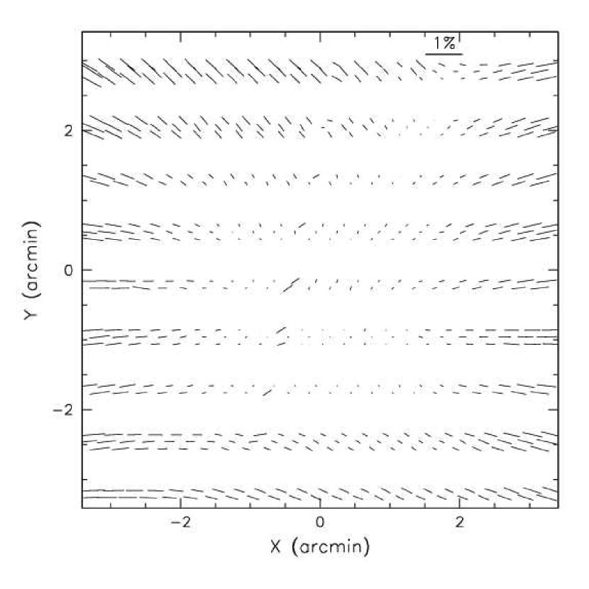
Figure 11.— Residual field obtained subtracting the ray-tracing model from the observed polarization in the $B$ band.

We must notice that our method heavily relies on the assumptions that the instrumental polarization is null on the optical axis and the sky background polarization is constant across the field of view. As a matter of fact, the night sky polarization is not very well studied. The only extensive analysis we could find in the literature is the one by Wolstencroft & Bandermann (1973), who concluded that the polarization structure varies in scale from a few degrees to about 30^∘, i.e. on scales which are much larger than the field of view of FORS1 (6′. 8 $\times$ 6′. 8). In order to explain the deviations we observe from a centrally symmetric pattern, one would need a variation in the sky polarization of the order 0.5% on a scale of a few arcmin. Even though this seems to be quite a large gradient, in principle we cannot exclude it. Only further tests will clarify the nature of the effect we see in the $B$ band.

12. Discussion and Conclusions

Dual-beam polarizers coupled to 2D arrays provide a tool to perform panoramic imaging polarimetry and multi-object spectro-polarimetry. In these instruments, the atmospheric fluctuations problem is solved by obtaining simultaneous measurements of two orthogonal polarization states. Of course, the use of a WP has also some drawbacks, as the flat-fielding issue discussed in Sec. 6. With the only exception of this feature, data reduction and analysis are totally similar to other polarimetric systems, as we have shown with both analytical and numerical approaches (Secs. 3 and 4).

When the targets to be studied are extended and cover a large fraction of the field-of-view, accurate background subtraction becomes an issue, whose effects we have investigated in Sec. 5. This is particularly important when the background is not the simple sky background, but it has a complicated structure. This is the case, for instance, for a faint supernova projected onto a galactic spiral arm.

Another problem that may reduce the performance of a dual-beam polarimeter is the imperfect behaviour of the WP. In Sec. 7 we have discussed this issue and presented a test to determine possible deviations from the ideal case. As an example, we have applied it to the FORS1 archive data we have described in Sec. 10. Using an object-free region roughly in the center of the field-of-view we have used Eqs. 14 and 15 to compute $t$ (see Eq. 12), which turns out to be $t$=0.502$\pm$0.001, i.e. perfectly compatible with the value derived from the Fourier analysis (Sec. 8). As we have shown, the redundancy introduced by having $N\geq 4$ strongly reduces this problem, even in the cases where $t$ differs by about 10% from the ideal case ($t$=0.5). This is the case also for the presence of linear polarization in the post-analyzer optics, whose effects are practically eliminated by the redundancy (Sec. 9).

Finally, we have addressed the instrumental polarization issue, described its consequences and proposed an easy test to detect any spurious effect with rather high accuracy (Sec. 10). As an example, we have applied it to archival FORS1 data and we have detected an instrumental polarization pattern, roughly centrally symmetric (for $V$ and $I$) and with a radial dependency. The presence of this spurious polarization affects all objects placed at distances larger than 1′. 5 from the optical axis with intrinsic polarizations of a few percent or less. The problem becomes particularly severe when $p\simeq P$: in that case the measured Stokes parameters can be severely wrong. For objects filling most of the field of view, there always will be regions affected by this problem. Moreover, the correct sky background estimate, which is absolutely necessary to recover the intrinsic object field in the outer parts of the galaxy, becomes impossible, if the instrumental polarization is not taken care of properly. The spurious field must be removed before one is able to estimate the background contribution. Both our data and ray-tracing simulations show that the effect is wavelength dependent. In the case of FORS1, a strong deviation from central symmetry is seen in the $B$ band and we have interpreted this as a signature of an additional effect, yet to be explained, not included in the ray-tracing simulations that, in contrast, reproduce quite well the observed data in $V$ and $I$.

One possible source of asymmetric instrumental polarization is the unrelieved stress birefringence in the optical glasses, due to thermal strain and mechanical loading (see for example Theocaris & Gdoutos, 1979). This phenomenon is known to introduce a retardance which, in turn, can change the polarization status of incoming polarized light (the effect is null if the light is unpolarized). Since the incoming radiation is certainly polarized by FORS1 in a differential way across the field of view, this would also imply that the secondary effect should be weaker where the centrally symmetric component is smaller. The fact that this is indeed the case (see Fig. 11) and also that the retardance is expected to grow faster than $\lambda^{-1}$ seem to suggest that this is a plausible explanation for the asymmetric component. If this is indeed the case, then it is not possible to correct the measured linear polarization just subtracting vectorially the residual field (like the one shown in Fig. 11) simply because the effect of retardance depends on the polarization state of the incoming light. This requires a more sophisticated treatment, necessarily based on the exact knowledge of the physical mechanism and its mathematical description through Mueller matrices formalism.

In general, instrumental polarization induced by transmission is most likely common to all focal reducers equipped with a polarimetric mode. While the overall pattern should be a general feature of these instruments, the exact radial dependence may change according to the optical design and the curvature of the lenses. The method we have described in this paper allows an accurate way of characterizing the instrument and a tool to correct for this effect.

References

- Appenzeller (1967) Appenzeller, I., 1967, PASP, 79, 136
- Avila (2005) Avila, G. 2005, ESO Technical Note INS-05/01
- Bagnulo et al. (2000) Bagnulo, S., Szeifert, T., Wade, G. A., Landstreet, J.D. & Mathys, G. 2000, A&A, 389, 191
- Born & Wolff (1980) Born, M. & Wolff, E. 1980, Principles of Optics, 6th ed., (New York: Pergamon Press)
- Chandrasekhar (1950) Chandrasekhar, S., 1950, Radiative Transfer, (Oxford: Oxford University Press)
- Clarke & Stewart (1986) Clarke, D. & Stewart. B.G. 1986, Vistas Astron., 29, 27
- Fendt et al. (1996) Fendt, C., Beck, R., Lesch, H. & Neninger, N. 1996, A&A, 308, 713
- Goldstein (2003) Goldstein, D. 2003, Polarized Light, second edition, (New York: Marcel Dekker Inc.)
- Keller (2002) Keller, C.U. 2002, in Astrophysical Spectropolarimetry, (Cambridge: Cambridge University Press, p.303)
- Kendall & Stuart (1977) Kendall, M. & Stuart, K. 1977, The Advanced Theory of Statistics, Vol. 1, (London: Charles Griffin & Co.)
- Leinert et al. (1998) Leinert, Ch., Bowyer, S., Haikala, L.K., et al. 1998, A&AS, 127, 1
- Leroy (2000) Leroy, J.L. 2000, Polarization of Light and Astronomical Observation, (Singapore: Gordon & Breach Science Publishers)
- McLean, Aspin & Reitsema (1983) McLean, I.S., Aspin, C. & Reitsema, H. 1983, Nature, 304, 243M
- McLean (1997) McLean, I.S. 1997, Electronic Imaging in Astronomy, John Wiley & Sons
- Miller, Robinson & Goodrich (1987) Miller, J.S., Robinson, L.B. & Goodrich, R.W. 1987, in Instrumentation for Ground-Based Optical Astronomy, Ed. L.B. Robinson, p.157
- Oliva (1997) Oliva, E. 1997, A&AS, 13, 589
- Patat (1999) Patat, F. 1999, EFOSC2 User’s Manual, LSO-MAN-ESO-36100-0004
- Pernechele et al. (2003) Pernechele, C., Giro, E., & Fantinel, D. 2003, SPIE Proc., 4843, 156
- Press et al. (1999) Press, W. H., Teukolsky, S. A., Vetterling, W. T., & Flannery, B. P. 1999, Numerical Recipes in C: the Art of Scientific Computing, 2nd ed., (Cambridge: Cambridge University Press)
- Rice (1944) Rice, S.O. 1944, Bell System Tech. J., 24,96
- Roach & Gordon (1973) Roach, F.E. & Gordon, J.L. 1973, The light of the Night Sky, (Dordrecht: D. Reidel Publ. Company)
- Scarrot et al. (1983) Scarrot, S.M., Warren-Smith, R.F., Pallister, W.S., Axon, D.J. & Bingham, R.G. 1983, MNRAS, 204, 1163
- Schmidt, Stockman & Smith (1992) Schmidt, G. D., Stockman, H. S. & Smith, P. S. 1992, ApJ, 398, L60
- Seifert (1994) Seifert, W. 1994, FORS Final Design Report - Optics, VLT-TRE-VIC-13110-0011
- Serkowski (1958) Serkowski, K. 1958, Acta Astron., 8, 135
- Shurcliff (1962) Shurcliff, W.A. 1962, Polarized Light, Production and Use (Cambridge: Harvard University Press)
- Simmons & Stewart (1985) Simmons, J.F.L. & Stewart, B.G. 1985, A&A, 142, 100
- Sparks & Axon (1999) Sparks, W. B. & Axon, D. J. 1999, PASP, 111, 1298
- Szeifert (2002) Szeifert, T. 2002, FORS1+2 User’s Manual, VLT-MAN-ESO-13100-1543, Issue 2.3
- Theocaris & Gdoutos (1979) Theocaris, P.S. & Gdoutos, E.E. 1979, Matrix Theory of Photoelasticity, Chap. 2 (Berlin: Springer-Verlag)
- Tinbergen (1996) Tinbergen, J. 1996, Astronomical Polarimetry, (Cambridge: Cambridge University Press)
- Wardle & Kronberg (1974) Wardle, J.F.C. & Kronberg, P.P. 1974, ApJ, 194, 249
- Wolstencroft & Bandermann (1973) Wolstencroft, R.D. & Bandermann, L.W. 1973, MNRAS, 163, 229