Observational Constraints on a Variable Dark Energy Model

Abstract

We study the effect of a phenomenological parameterized quintessence model on low, intermediate and high redshift observations. At low and intermediate redshifts, we use the Gold sample of supernova Type Ia (SNIa) data and recently observed size of baryonic acoustic peak from Sloan Digital Sky Survey (SDSS), to put constraint on the parameters of the quintessence model. At the high redshift, the same fitting procedure is done using WAMP data, comparing the location of acoustic peak with that obtain from the dark energy model. As a complementary analysis in a flat universe, we combine the results from the SNIa, CMB and SDSS. The best fit values for the model parameters are $\Omega_{m}=0.27^{+0.02}_{-0.02}$ (the present matter content) and $w_{0}=-1.45^{+0.35}_{-0.60}$ (dark energy equation of state). Finally we calculate the age of universe in this model and compare it with the age of old stars and high redshift objects.

PACS numbers: 05.10.-a ,05.10.Gg, 05.40.-a, 98.80.Es, 98.70.Vc

]

I Introduction

Observations of the apparent luminosity and redshift of type Ia supernovas (SNIa) provided us with the main evidence for the accelerating expansion of the Universe [1, 2]. A combined analysis of SNIa and the Cosmic Microwave Background radiation (CMB) observations indicates that the dark energy fills about $2/3$ of the total energy of the Universe and the remaining part is the dark matter and a few percent in the Baryonic form [3, 4, 5].

The ”cosmological constant” which was introduced by Einstein to have a static universe, can be a possible solution for the acceleration of the universe [6]. The cosmological constant in Einstein field equation is a geometrical term, however, it can be regarded as a fluid with the equation of state of $w=-1$. There are two problems with this scenario, namely the two dark energy problems of the fine-tuning and the cosmic coincidence. Within the framework of quantum field theory, the vacuum expectation value of the energy momentum tensor diverges as $k^{4}$. A cutoff at the Planck energy leads to a cosmological constant with $123$ orders of magnitude larger than the observed value of $10^{-47}$ GeV⁴. The absence of a fundamental mechanism which sets the cosmological constant to zero or to a very small value is the cosmological constant problem. The second problem, cosmic coincidence, states that since the energy densities of dark energy and dark matter scale so differently during the expansion of the Universe, why are they nearly equal today?

One of the solutions to this problem is a model with decaying cosmological constant from the Planckian area at the early Universe to a small enough at the present time. Dolgov (1983) proposed a massless non-minimally coupled scalar field to the gravity with a negative coupling constant to solve this problem [7]. However, this model provides a time varying Gravitational constant which strongly contradicts the upper limits from the Viking radar range [8] and lunar laser ranging experiments [9]. A non-dissipative minimally coupled scalar field, so-called Quintessence model can also play the role of time varying cosmological constant [10, 11, 12]. The ratio of energy density of this field to the matter density increases by the expansion of the universe and after a while the dark energy becomes the dominated term in the energy-momentum tensor. Tuning the parameters of this model it can produce the value of $\Lambda$-term both for the early universe and the present time.

One of the features of the quintessence model is the evolution of the equation of state of dark energy during the expansion of the Universe. Various models depending on the potential for the scalar field as k-essence [13], Tachyonic matter [14], Phantom [15, 16] and Chaplygin gas [17] provide different time dependent functions for the equation of state [16, 18, 19, 20, 21, 22, 23, 24]. There are also phenomenological models, parameterize the equation of state of dark energy in terms of redshift [25, 26, 27]. Here we examine a simple phenomenological parameterization for the variable dark energy, proposed by Wetterich (2004) [28]. In this parameterization the variable dark energy is expressed in terms of three parameters. The first two parameters are the dark energy density, $\Omega_{\lambda}$ and dark energy equation of state $w_{0}$ at the present time. The third parameter $b$ is the bending parameter which can be expressed in terms of the fraction of dark energy at early universe. The equation of state of this model depends on $b$ and $w_{0}$ as:

$$w(z;b,w_{0})=\frac{w_{0}}{\left[1+b\ln(1+z)\right]^{2}},$$ (1)

Using the continuity equation, the density of dark energy changes with the redshift as:

$$\rho_{\lambda}(z;b,w_{0})=\rho_{\lambda}(1+z)^{3[1+\bar{w}(z;b,w_{0})]},$$ (2)

where $\bar{w}(z;b,w_{0})={w_{0}}/\left[1+b\ln(1+z)\right]$. In this paper we compare this model in a flat universe with the cosmological observations such as SNIa, CMB shift parameter and Large Scale Structure (LSS) and constrain the parameters of the model.

The organization of the paper is as follows: In Sec. II we study the effect of the parameters of the dark energy model on the age of Universe, comoving distance, comoving volume element and the variation of angular size by the redshift [29]. In Sec. III we use the Gold sample of Supernova Type Ia data [30] to constrain the parameters of the model. In Sec. IV the position of the observed acoustic angular scale on CMB is compared with that of quintessence model. In Sec. V with the combined SNIa$+$ CMB$+$ SDSS data we put better constraints on the parameters of this model. Finally the age of the universe determined by this model is compared with the age of the old stars and old high redshift objects as the consistency test. The conclusions are given in Sec. VI.

II the effect of variable dark energy on the geometrical parameters

In this section we study the geometrical effect of the dark energy on the observable parameters of the universe as itemized as follows:

• comoving distance: The radial comoving distance of an object located at a given redshift $z$ is one of the basis parameters of the cosmology. Using the null geodesics in the FRW metric, the comoving distance can be obtained by:

  $$r(z;b,w_{0})=\int_{0}^{z}{dz^{\prime}\over H(z^{\prime};b,w_{0})},$$ (3)

  where $H(z;b,w_{0})$ is the Hubble parameter and for the redshifts smaller than the radiation dominant epoch $(z<z_{eq})$, it can be expressed in terms of Hubble parameter at the present time, $H_{0}$, the matter and dark energy content of the universe as:

  $$H^{2}(z;b,w_{0})=H_{0}^{2}[\Omega_{m}(1+z)^{3}+\Omega_{\lambda}(1+z)^{3[1+\bar{w}(z)]}],$$ (4)

  

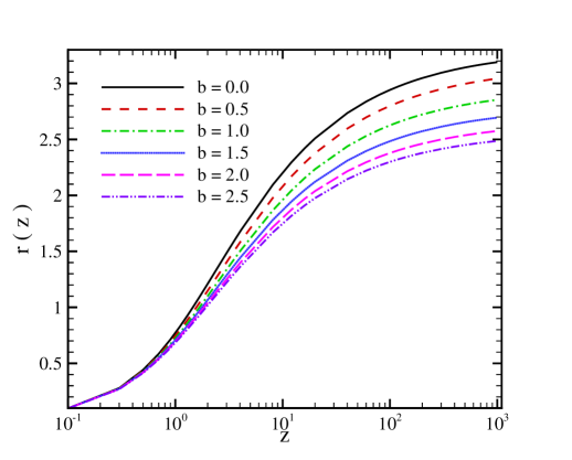
  FIG. 1.: Comoving distance, $r(z;b,w_{0})$ (in unit of $c/H_{0}$) as a function of redshift for various values of bending parameters.

  By numerical integration of equation (3), the comoving distance as a function of redshift can be obtained. The dependence of comoving distance in terms of redshift for various bending factors is shown in Figure 1. This diagram shows that the comoving distance is more sensitive to $b$ at higher redshifts than lower redshifts. Increasing the bending parameter leads the dark energy dominance at the higher redshifts which results a slow growth of $r(z;b,w_{0})$. For redshifts around $z=0$ we can expand equation (3) as:

  $$r(z)=H_{0}^{-1}\left[z-{3\over 4}z^{2}(1+\Omega_{\lambda}w_{0})+\frac{\Omega_{\lambda}w_{0}}{2}bz^{3}+\cdots\right].$$ (5)

  One of the main applications of the comoving distance is in the luminosity distance calculation. In the next section we use SNIa data as the standard candle in the cosmological scales to confine the parameters of the dark energy model.

• angular size: The apparent angular size of objects at the cosmological scales is another observable that can be affected by the dark energy model. If $D$ is the physical size of an object that subtends an angle $\theta$ to the observer, for small $\theta$ we have:

  $$D=d_{A}\theta$$ (6)

  where $d_{A}=r(z;b,w_{0})/(1+z)$ is called the angular diameter distance. One of the main applications of equation (6) is on measurement of matter content of the universe by observing the apparent angular size of acoustic peak on CMB map and baryonic acoustic peak at lower redshifts. A variable dark energy can change the comoving distance to the observer and consequently the apparent size of the acoustic peak. So measurement of the angular size of objects in various redshifts (so-called Alcock-Paczynski test) can probe the variable dark energy [29]. The variation of apparent angular size $\Delta\theta$ in terms variations of redshift $\Delta z$ can be determined as:

  $${\Delta z\over\Delta\theta}=\frac{H(z;b,w_{0})r(z;b,w_{0})}{\theta}$$ (7)

  

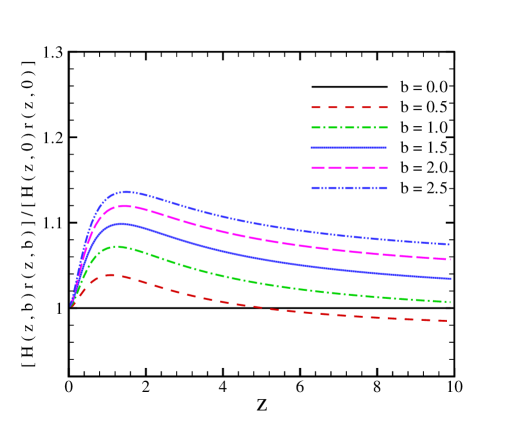
  FIG. 2.: Alcock-Paczynski test, compares $\Delta z/{\Delta\theta}$ normalized to the case of $\Lambda$CDM model as a function of redshift.

  Figure 2 shows $\Delta z/\Delta\theta$ in terms of redshift, normalized to the case with $b=0$ ($\Lambda$CDM model). According to Figure 2, the variation of the apparent angular size is sensitive to the bending parameter at higher redshifts. The advantage of Alcock-Paczynski test is that we need standard ruler in the universe instead of the standard candle. Recently a possible Alcock-Paczynski test for measuring the dark energy parameters has been proposed by high-z observation of the power spectrum of large scale structures at 21cm wavelength. Observation of 21cm fluctuations will enable us to determine the angular diameter and the Hubble constant [31, 32]. The Ly-$\alpha$ forest of close QSO pairs may also measure $\Omega_{\lambda}$ and its variation with time [33].

• comoving volume element: The other geometrical parameter is the comoving volume element which is the basis of number-count tests, such as lensed quasars, galaxies, or clusters of galaxies. The comoving volume element in terms of comoving distance and Hubble parameters is given by:

  $$f(z;b,w_{0})\equiv{dV\over dzd\Omega}=r^{2}(z;b,w_{0})/H(z;b,w_{0}).$$ (8)

  As shown in Figure 3, the comoving volume element reaches to its maximum value around $z\simeq 2$ and for larger bending parameters the position of the peak shifts to the smaller redshifts.

  

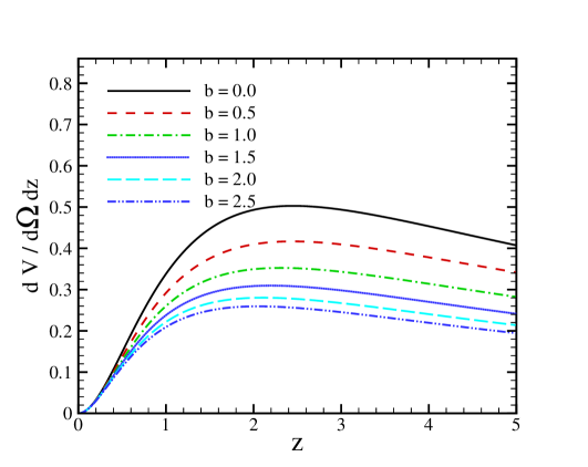
  FIG. 3.: The comoving volume element in terms of redshift for various bending parameters. Increasing the bending parameters makes the position of maximum value of volume element shifts to the smaller redshifts.

• age of the universe: The age of universe is another observable parameter that can be used to constrain the parameters of dark energy models. Studies on the old stars [34] suggests an age of $13^{+4}_{-2}$ Gyr for the universe. Richer et. al. [35] and Hansen et. al. [36] also proposed an age of $12.7\pm 0.7$ Gyr, by using the white dwarf cooling sequence method. For a detailed review on the cosmic age see [5]. The universe age in varying dark energy models depends on the parameters of the model. Integrating the age of universe from the beginning of universe up to now, we obtain the age of universe as follows:

  $$t_{0}(b,w_{0})=\int_{0}^{t_{0}}\,dt=\int_{0}^{\infty}{dz\over(1+z)H(z;b,w_{0})},$$ (9)

  Similarly to the effect of bending parameter on the comoving distance, in the case of age of the universe, increasing the bending parameter makes a shorter age for the universe. Figure 4 shows the effect of bending parameter on the age of universe. Here we show the variation of $H_{0}t_{0}$ as a function of $b$ for a typical values of cosmological parameters (e.g. $h=0.65$, $\Omega_{m}=0.27$ and $w_{0}=-1.0$).

  

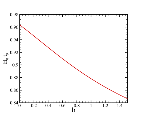
  FIG. 4.: Age times Hubble constant as the present time $(H_{0}t_{0})$, as a function of $b$ in a flat universe with the parameters of $\Omega_{m}=0.3$, $h=0.65$ and $w_{0}=-1.0$. Increasing bending parameters makes a shorter age for the universe.

III Test by Supernova Type Ia: Gold Sample

The Supernova Type Ia experiments provided the main evidence for the existence of dark energy in the framework of standard cosmology. Since 1995 two teams of the High-Z Supernova Search and the Supernova Cosmology Project have been discovered several type Ia supernova candidates at the high redshifts [20, 37]. Recently Riess et al.  (2004) announced the discovery of $16$ type Ia supernova with the Hubble Space Telescope. This new sample includes $6$ of the $7$ most distant ($z>1.25$) type Ia supernovas. They determined the luminosity distance of these supernovas and with the previously reported algorithms, obtained a uniform Gold sample of type Ia supernovas, containing $157$ objects [30, 38, 39]. In this section we compare the distance modulus of the Gold sample data with that theoretically derived from the dark energy model. The distance modulus $(\mu=m-M)$ in terms of redshift and parameters of model is given by:

$$m-M=5\log{D_{L}(z;b,w_{0})}+25,$$ (10)

where $M$ is the absolute magnitude, $D_{L}$ is the luminosity distance in Mpc and $m$ is the corrected apparent magnitude, including reddening, K correction etc. For a flat and homogeneous cosmological model the luminosity distance can be obtained by:

$$D_{L}(z;b,w_{0}) = (1+z)\int^{z}_{0}{dz^{\prime}\over H(z^{\prime};b,w_{0})}.$$ (11)

The comparison between the observed and theoretical distance modulus is given by $\chi^{2}$ as follows:

$$\chi^{2}=\sum_{i}^{N}\frac{[\mu_{obs}(z_{i})-\mu_{th}(z_{i};\Omega_{m},w_{0},b,h)]^{2}}{\sigma_{i}^{2}},$$ (12)

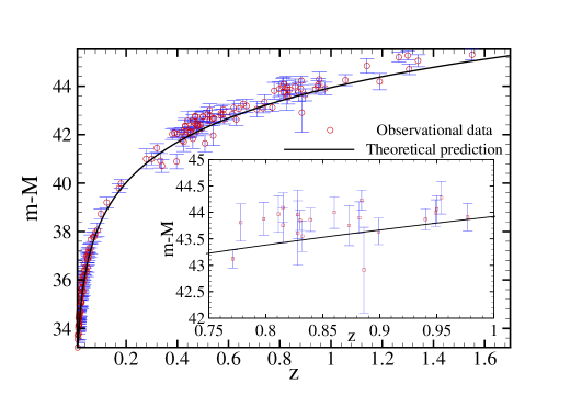
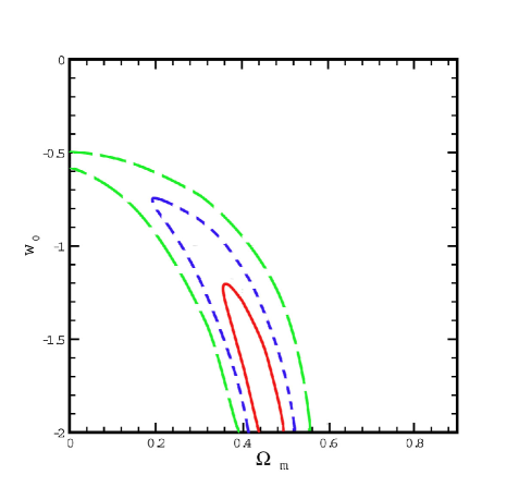
where $\sigma_{i}$ is the error bar of the observed distance modulus for each Supernova candidate. The best fit values for the model parameters are $w_{0}=-1.90_{-3.29}^{+0.75}$, $\Omega_{m}=0.01^{+0.51}_{-0.01}$ and $b=6.00_{-6.00}^{+7.35}$ with $\chi^{2}_{min}/N_{d.o.f}=1.13$ at $1\sigma$ level of confidence. Figure 5 compares the distance modulus of the observed SNIa Gold sample in terms of redshift and the best fit from the dark energy model. We see clearly that the fit values in this model are evidently different from those of $\Lambda$CDM (the WMAP results for $\Lambda$CDM models are: $h=0.71^{+0.04}_{-0.03}$ and $\Omega_{m}=0.27^{+0.04}_{-0.04}$ [5, 40]). We also compare our result with that of Riess et al. (2004), putting $b=0$ we should recover their result. Figure 6 indicates the confidence contours of $1\sigma$, $2\sigma$ and $3\sigma$ in the $(\Omega_{m},w_{0})$ plane for the case of $b=0$, marginalized over $h$, shows a good agreement with that of Riess et al. (2004).

By substituting the cosmological parameters derived from the SNIa fit in equation (9), we obtain the age of universe about $13.45$ Gry, which is in good agreement with the age of old stars.

FIG. 5.: Comparison of the distance modulus of the SNIa Gold sample in terms of redshift with the dark energy model. Solid line shows the best fit ($\chi^{2}_{min}/N_{d.o.f}=1.13$) with the corresponding parameters of $w_{0}=-1.90_{-3.29}^{+0.75}$, $\Omega_{m}=0.01^{+0.51}_{-0.01}$ and $b=6.00_{-6.00}^{+7.35}$ in $1\sigma$ level of confidence.

FIG. 6.: Joint confidence intervals for $\Omega_{m}$ and $w_{0}$ for the case of $b=0$ with $1\sigma$ (solid-line), $2\sigma$ (dashed-line) and $3\sigma$ (long dashed-line) confidence level. This result is in good agreement with that of Riess et al. (2004).

IV The location of acoustic peak on CMB Map

In this section we use the CMB data from the WMAP experiment to put additional constraints on the parameters of the dark energy model [41]. The statistical properties of the temperature fluctuations on CMB is given by a two point correlation function. In the isotropic universe, the two point correlation function $C(\gamma)$ depends only on the angle between the two vectors $(\gamma)$ connecting the observer to the last scattering surface and it can be expanded into a Legendre polynomials as:

$$C(\gamma)\,=\,\frac{1}{4\pi}\sum_{l=2}^{\infty}(2l+1)C_{l}P_{l}(\cos{\gamma}),$$ (13)

where $C_{l}$ is the widely used angular power spectrum. The summation over $l$ starts from $2$ because the $l\,=\,0$ term is the monopole which in the case of statistical isotropy the monopole is constant, and it can be subtracted out. The dipole $l\,=\,1$ is due to the local motion of the observer with respect to the last scattering surface and can be subtracted out as well.

The relevant parameter in the spectrum of CMB which can determine the geometry and matter content of universe is the position of the apparent acoustic peak. The acoustic peak corresponds to the Jeans length of photon-baryon structures at the last scattering surface some $\sim 379$ Kyr after the Big Bang [5]. The position of the acoustic peak in Legendre polynomial space relates to its apparent angular size, $\theta_{A}$ through $l_{A}\equiv\pi/\theta_{A}$. The apparent angular size of acoustic peak in a flat universe can be obtained by dividing of the comoving sound horizon at the decoupling epoch $r_{s}(z_{dec})$ to the comoving distance of observer to the last scattering surface $r(z_{dec})$ as:

$$\theta_{A}={{r_{s}(z_{dec})}\over r(z_{dec})},$$ (14)

where we take the redshift of the decoupling at $z_{dec}=1089$ [42]. The sound horizon corresponds to a distance that a perturbation of pressure can travel from the beginning of universe up to the decoupling area. The size of sound horizon at numerator of equation (14) can be obtained by:

$$r_{s}(z_{dec};b,w_{0})=\int_{z_{dec}}^{\infty}\frac{v_{s}(z)}{H(z;b,w_{0})}dz$$ (15)

where $v_{s}(z)^{-2}=3+9/4\times\rho_{b}(z)/\rho_{r}(z)$ is the sound velocity in the unit of speed of light from the big bang up to the last scattering surface [22, 42]. The denominator of equation (14), $r(z_{dec})$, comoving distance to the last scattering surface is also given by equation (3).

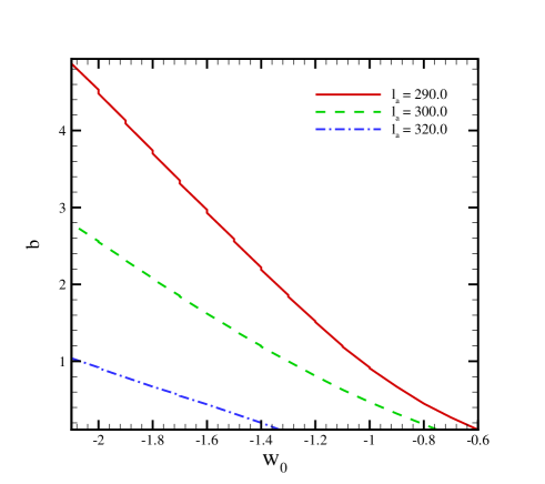
Changing parameters of the dark energy can shift the size of apparent acoustic peak and the position of $l_{A}$ in the power spectrum. Here we plot the dependence of $l_{A}$ on $b$ and $w_{0}$ for a typical values of cosmological parameters (Figure 7). It is seen that increasing $b$ makes a shorter comoving distance to the last scattering surface (see Figure 1) and subsequently results in a larger acoustic size or smaller $l_{A}$. By a similar argument as in the case of $b$, shifting $w_{0}$ towards zero makes smaller $l_{A}$.

FIG. 7.: Dependence of acoustic angular scale $l_{A}$ on the bending parameter, $b$ and $w_{0}$ for the three cases of $l_{A}=290$ (solid-line), $300$ (dashed-line) and $320$ (dashed-dotted line).

In order to compare the angular size of acoustic peak from this model with the observation we use the shift parameter as [43]:

$$R=\sqrt{\Omega_{m}}\int_{0}^{z_{dec}}\frac{dz}{E(z;b,w_{0})},$$ (16)

where $E(z;b,w_{0})=H(z;b,w_{0})/H_{0}$. The shift parameter is proportional to the size of acoustic peak to that of flat pure-CDM, $\Lambda=0$ model, ($R\propto\theta_{A}/\theta_{A}^{\it flat}=l_{A}^{\it flat}/l_{A}$). The observational result of CMB experiments correspond a shift parameter of $R=1.716\pm 0.062$ (given by WMAP, CBI, ACBAR) [5, 40]. One of the advantages of using the parameter $R$ is that it is independent of the Hubble constant. The best fit values for the dark energy model using the combined CMB and SNIa observations, minimizing $\chi^{2}=\chi^{2}_{{\rm SNIa}}+\chi^{2}_{{\rm CMB}}$, results in: $\Omega_{m}=0.37^{+0.08}_{-0.07}$, $b=2.7^{+5.25}_{-1.65}$ and $w_{0}=-2.5^{+0.90}_{-2.85}$ with $\chi_{min}/N_{d.o.f}=1.11$ with ($1\sigma$) level of confidence (see Table I). The age of universe from these parameters is $13.47$ Gyr.

In the next section we use the additional LSS data from SDSS and combine them with that of CMB and SNIa, to put more constraint on the parameters of the dark energy model.

V LSS Combined analysis with the CMB and SNIa

Recent observations of large scale correlation function measured from the spectroscopic sample of 46,748 Luminous Red Galaxies (LRG) by the Sloan Digital Sky Survey shows a well detected peak around $100$ Mpc $h^{-1}$.

This peak is an excellent match with the predicted shape and the location of the imprint of the recombination-epoch acoustic oscillation on the low-redshift clustering matter [44]. For a flat universe we can construct parameter $A$ as follows:

$$A=\sqrt{\Omega_{m}}E(z_{1};b,w_{0})^{-1/3}\times\left[\frac{1}{z_{1}}\int_{0}^{z_{1}}\frac{dz}{E(z;b,w_{0})}\right]^{2/3},$$ (17)

where $E(z;b,w_{0})=H(z;b,w_{0})/H_{0}$. Here $A$ is also independent of $H_{0}$. We use the robust constraint on the dark energy model using the value of $A=0.469\pm 0.017$ from the LRG observation at $z_{1}=0.35$ [44].

In what follows we perform a combined analysis of SNIa, CMB and SDSS to constrain the parameters of dark energy model. The combined $\chi^{2}$ from each experiment is as follows:

$$\chi^{2}=\chi^{2}_{\rm{SNIa}}+\chi^{2}_{{\rm CMB}}+\chi^{2}_{{\rm SDSS}},$$ (18)

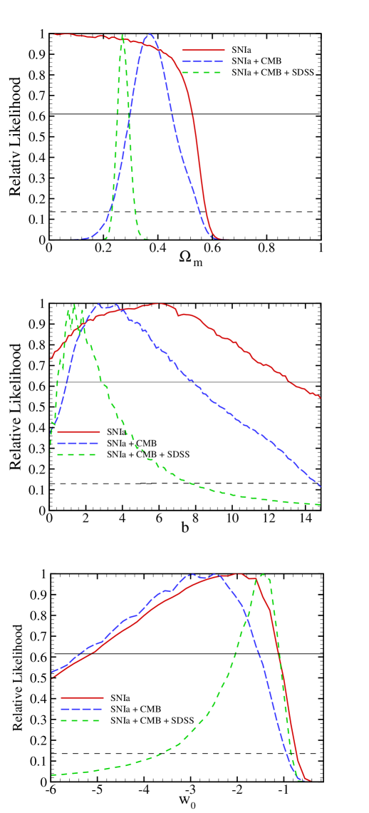
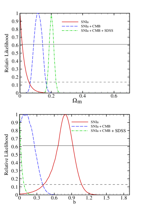
where $\chi^{2}_{{\rm SNIa}}$ is obtained from equation (12), comparing the distance modulus of the SNIa candidates from the Gold sample with that of theoretical dark energy model. $\chi^{2}_{{\rm CMB}}$ is also calculated by comparison of the observed shift parameter by WMAP with the model through equation (16) and finally $\chi^{2}_{{\rm SDSS}}$ is obtained from equation (17). The marginalized likelihood functions $(\mathcal{L}$$\propto e^{-\chi^{2}/2})$ [45] in terms of the parameters of the model for three cases of (i) fitting model with Supernova data, (ii) with SNIa$+$CMB data and (iii) considering all three experiments of CMB$+$SNIa$+$SDSS are shown in Figure 8.

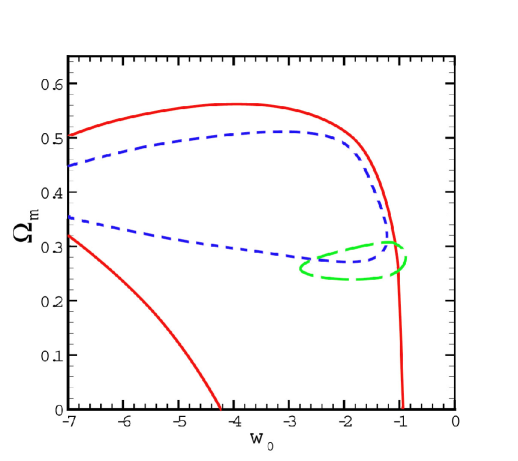
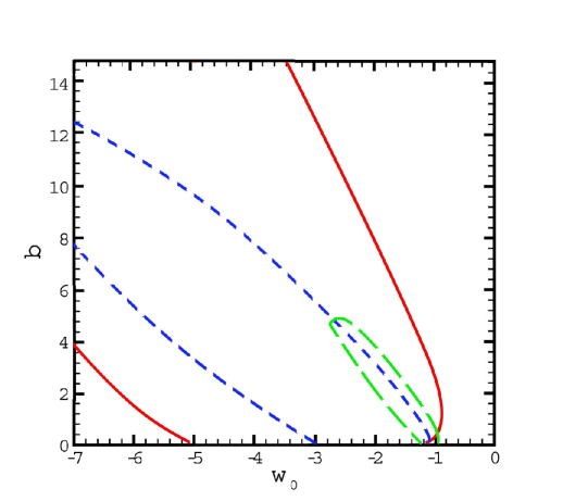
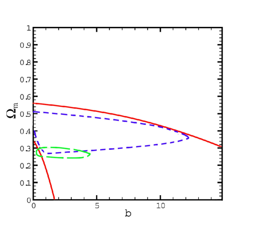
The best fit values for the model parameters by marginalizing on the remained ones are: $\Omega_{m}=0.27_{-0.02}^{+0.02}$, $b=1.35_{-0.90}^{+1.65}$ and $w_{0}=-1.45_{-0.60}^{+0.35}$ at $1\sigma$ confidence level with $\chi^{2}_{min}/N_{d.o.f}=1.11$. Table I indicates the corresponding values for the cosmological parameters from this fitting with one and two $\sigma$ level of confidence. The joint confidence contours in the $(w_{0},\Omega_{m})$, $(w_{0},b)$ and $(b,\Omega_{m})$ planes are shown in Figures 9, 10 and 11. Comparing Figure 6 which corresponds to the fitting with SNIa, prior $b=0$ with the solid contour in Figure 9, shows that adding the $b$ parameter increases the degeneracy between $\Omega_{m}$ and $w_{0}$.

TABLE I.: The best values for the parameters of variable dark energy as $\Omega_{m}$, $b$, $w_{0}$ with the corresponding age for the universe from the fitting with the SNIa, SNIa+CMB and SNIa+CMB+SDSS experiments with $1\sigma$ and $2\sigma$ confidence level.

Observation	$\Omega_{m}$	$b$	$w_{0}$	age
				(Gyr)
	$0.01^{+0.51}_{-0.01}$	$6.00^{+7.35}_{-6.00}$	$-1.90^{+0.75}_{-3.29}$
SNIa				$13.45$
	$0.01^{+0.56}_{-0.01}$	$6.00^{+17.42}_{-6.00}$	$-1.90^{+1.10}_{-7.23}$
	$0.37^{+0.08}_{-0.07}$	$2.70^{+5.25}_{-1.65}$	$-2.50^{+0.90}_{-2.85}$
SNIa$+$CMB				$13.47$
	$0.37^{+0.18}_{-0.15}$	$2.70^{+11.85}_{-2.70}$	$-2.50^{+1.50}_{-6.71}$
SNIa$+$CMB	$0.27^{+0.02}_{-0.02}$	$1.35^{+1.65}_{-0.90}$	$-1.45^{+0.35}_{-0.60}$
$+$SDSS				$14.09$
	$0.27^{+0.04}_{-0.03}$	$1.35^{+6.30}_{-1.35}$	$-1.45^{+0.65}_{-2.10}$

We repeat the same analysis for the special case, fixing $w_{0}=-1.0$. The best fit values for the parameters of the model in this case obtain as $\Omega_{m}=0.28_{-0.02}^{+0.02}$, $b=0.24_{-0.23}^{+0.27}$ at $1\sigma$ confidence level with $\chi^{2}_{min}/N_{d.o.f}=1.12$. For the case of using the result of HST-Key project (Hubble parameter $h=0.71\pm 0.07$), the marginalized likelihood function in this special case, where we have two free parameters of $\Omega_{m}$ and $b$ are shown in Figure 12. The best fit values for the model parameters are: $\Omega_{m}=0.20_{-0.01}^{+0.01}$, $b=0.00_{-0.00}^{+0.02}$ at $1\sigma$ confidence level with $\chi^{2}_{min}/N_{d.o.f}=1.75$. In this case we have almost $\Lambda$CDM model with no variation in the equation of state of dark energy.

Finally we do the consistency test, comparing the age of universe derived from this model with the age of old stars and the age of Old High Redshift Galaxies (OHRG) in various redshifts. One of the reasons for the existence of the dark energy is the problem of ”age crisis”, i.e. the universe without cosmological constant is younger than its constituents [46]. From Table I, we see that the age of universe from the combined analysis of SNIa$+$CMB$+$SDSS is $14.09$ Gyr which is in agreement with the age of old stars [34]. Here we take three OHRG for comparison with the dark energy model, namely the LBDS $53$W$091$, a $3.5$-Gyr-old radio galaxy at $z=1.55$ [46], the LBDS $53$W$069$, a $4.0$-Gyr-old radio galaxy at $z=1.43$ [47] and a quasar, APM $08279+5255$ at $z=3.91$ with an age of $t=2.1_{-0.1}^{+0.9}$Gyr [48]. The later one has once again led to the ”age crisis”. An interesting point about this quasar is that it cannot be accommodated in the $\Lambda$CDM model [49]. To quantify the age consistency test we introduce the expression $\tau$ as:

$$\tau=\frac{t(z;b,w_{0})}{t_{obs}}=\frac{t(z;b,w_{0})H_{0}}{t_{obs}H_{0}},$$ (19)

where $t(z)$ is the age of universe which can be obtained from the equation (9) and $t_{obs}$ is an estimation for the age of old cosmological object. In order to have a compatible age for the objects, we should have $\tau>1$.

Table II shows the value of $\tau$ for three mentioned OHRG. Various observational constraints on the parameters of the dark energy model from SNIa, CMB, LSS and their combinations, results an age for the universe more than the age of LBDS $53$W$069$ and LBDS $53$W$091$, while APM $08279+5255$ at $z=3.91$ is older than the age of universe. Only in the case that we fix $w_{0}=-1$ and use the SNIa+HST constraints, we obtain $\tau=1.26$, a compatible age for the universe with that of Quasar.

TABLE II.: The value of $\tau$ for three high redshift objects, using the parameters of the dark energy model from the best fit.

Observation	LBDS $53$W$069$	LBDS $53$W$091$	APM
			$08279+5255$
	$z=1.43$	$z=1.55$	$z=3.91$
SNIa	$1.13$	$1.21$	$0.78$
, $(w_{0}=-1)$
SNIa+HST	$1.67$	$1.81$	$1.26$
, $(w_{0}=-1)$
SNIa$+$CMB
$+$SDSS	$1.18$	$1.27$	$0.82$
, $(w_{0}=-1)$
SNIa$+$CMB
$+$SDSS	$1.29$	$1.38$	$0.89$
$+$HST,
$(w_{0}=-1)$
SNIa	$1.00$	$1.05$	$0.65$
SNIa$+$CMB	$1.09$	$1.17$	$0.75$
$+$SDSS

FIG. 8.: Marginalized likelihood functions of three cosmological parameters. The solid line is the likelihood function fitting the model with SNIa data, the long dashed-line with the joint SNIa$+$CMB and the dashed-line corresponds to the fitting with SNIa$+$CMB$+$SDSS data. The intersections of the curves with the horizontal solid and dashed lines give the bounds with $1\sigma$ and $2\sigma$ level of confidence respectively.

FIG. 9.: Joint confidence intervals for $\Omega_{m}$ and $w_{0}$ from fitting with the SNIa (solid line), SNIa$+$CMB (dashed-line) and SNIa$+$CMB$+$SDSS (long dashed-line) data with $1\sigma$ level of confidence.

FIG. 10.: Joint confidence intervals for $b$ and $w_{0}$ from fitting with the SNIa (solid line), SNIa$+$CMB (dashed-line) and SNIa$+$CMB$+$SDSS (long dashed-line) data with $1\sigma$ level of confidence.

FIG. 11.: Joint confidence intervals for $\Omega_{m}$ and $b$ from fitting with the SNIa (solid line), SNIa$+$CMB (dashed-line) and SNIa$+$CMB$+$SDSS (long dashed-line) data with $1\sigma$ level of confidence.

VI Conclusion

In this work we examined a parameterized quintessence model proposed by Wetterich (2004)[28] in a flat universe with the low, intermediate and high redshift observations. The effect of this model on the age of universe, radial comoving distance, comoving volume element and the variation of apparent size of objects with the redshift (Alcock-Paczynski test) have been studied.

In order to constrain the parameters of model we used the Gold sample SNIa data. The supernova analysis results in a large degeneracy between the parameters of the model. To improve the analysis, we combined analysis of SNIa and CMB shift parameter. Finally we used the results of recently observed baryonic peak at the Large Scale Structure, combined with the two former experiments to confine the parameters of the dark energy model. The fitting parameters from the joint analysis of SNIa$+$CMB $+$ SDSS marginalizing on the remained ones results in: $\Omega_{m}=0.27_{-0.02}^{+0.02}$, $b=1.35_{-0.90}^{+1.65}$ and $w_{0}=-1.45_{-0.60}^{+0.35}$ at $1\sigma$ confidence level with $\chi^{2}_{min}/N_{d.o.f}=1.11$. The best fit value for the equation of state of the dark energy leads to $w_{0}<-1$ which violates the strong energy condition. From the quantum field theory point of view, exotic models like scalar field with negative kinetic energy can provide $w<-1$ [50, 51] (theoretical attempts for $w<-1$ can be found in  [52, 53, 54, 55, 56])

FIG. 12.: Marginalized likelihood functions for two cosmological parameters of $\Omega_{m}$ and $b$ in the special case of fixing $w_{0}=-1$ and using the $H_{0}=71.0\pm 7.0$ from the HST-Key project.The solid line corresponds to the Likelihood function of the parameters for the case of fitting dark energy model with the SNIa data, the dashed line corresponds to the combined SNIa$+$ CMB data and dotted-dashed line is for combined SNIa$+$CMB$+$SDSS data. The intersections with the horizontal solid and dashed lines give the bounds for $1\sigma$ and $2\sigma$ confidence level respectively.

We also did the age test, comparing the age of old stars and old high redshift galaxies with the age that we obtained based on the dark energy model. The age of the universe from the best fit parameters of the model, results in an age of $14.09$ Gyr for the universe which is in agreement with the age of old stars. We also chose two high redshift radio galaxies at $z=1.55$ and $z=1.43$ with a quasar at $z=3.91$. The two first objects were consistent with the age of the universe, meaning that there were younger than the age of universe at the corresponding redshifts while the latter one was older than the age of universe. The age of APM $08279+5255$ quasar as the ”age crisis” was not compatible with the age of universe in this dark energy model. Only in the case that we fixed $w_{0}=-1$ and took $H_{0}=71.0\pm 7.0$ a compatible age for the universe with that of quasar has been obtained.

Acknowledgements The authors thank the anonymous referee for useful comments. This paper is dedicated to Dr. Somaieh Abdolahi.

REFERENCES

- [1] A. G. Riess et al., Astron. J. 116, 1009 (1998).
- [2] S. Perlmutter et al., Astrophys. J. 517, 565 (1999).
- [3] C. L. Bennett et al., Astrophys. J. Suppl. Ser. 148, 1 (2003).
- [4] H.V. Peiris et al., Astrophys. J. Suppl. Ser. 148, 213 (2003).
- [5] D. N. Spergel, L. Verde, H. V. Peiris et al., Astrophys. J. 148, 175 (2003).
- [6] S. Weinberg, Rev. Mod. Phys. 61, 1 (1989; S. M. Carroll, Living Rev. Relativity 4, 1 (2001); P. J. E. Peebles and B. Ratra, Rev. Mod. Phys. 75, 559 (2003); T. Padmanabhan, Phys. Rep. 380, 235 (2003).
- [7] A. D. Dolgov, in The very early universe, eds. G. W. Gibbons, S. W. Hawking and S. T. C.Siklos, Cambridge university press, Cambridge, 449 (1983).
- [8] R. W. Hellings et al., Phys. Rev. Lett. 51, 1609 (1983).
- [9] J. G. Williams, X. X. Newhall and J. O. Dickey , Planetary & Space Science 44, 1077 (1996).
- [10] C. Wetterich, Nucl. Phys. B302, 668 (1988); P. J. E. Peebles and B. Ratra, Astrophys. J. 325, L17 (1988); B. Ratra and P. J. E. Peebles, Phys. Rev. D 37, 3406 (1988); J. A. Frieman, C. T. Hill, A. Stebbins, and I. Waga, Phys. Rev. Lett. 75, 2077 (1995); M. S. Turner and M. White, Phys. Rev. D 56, R4439 (1997); R. R. Caldwell, R. Dave, and P. J. Steinhardt, Phys. Rev. Lett. 80, 1582 (1998); A. R. Liddle and R. J. Scherrer, Phys. Rev. D 59, 023509 (1999); I. Zlatev, L.Wang, and P. J. Steinhardt, Phys. Rev. Lett. 82, 896 (1999); P. J. Steinhardt, L. Wang, and I. Zlatev, Phys. Rev. D 59, 123504 (1999); D. F. Torres, Phys. Rev. D 66, 043522 (2002).
- [11] L. Amendola, Phys. Rev. D 62, 043511 (2000); L. Amendola and D. Tocchini-Valentini, Phys. Rev. D 64, 043509 (2001); 66, 043528 (2002); L. Amendola, Mon. Not. R. Astron. Soc. 342, 221 (2003); M. Pietroni, Phys. Rev. D 67, 103523 (2003); D. Comelli, M. Pietroni, and A. Riotto, Phys. Lett. B 571, 115 (2003); U. Franca and R. Rosenfeld, Phys. Rev. D 69, 063517 (2004); X. Zhang, astro-ph/0503072; Phys. Lett. B 611, 1 (2005).
- [12] P. J. E. Peebles, R. Ratra, Astrophys. J. 325, L17 (1988).
- [13] C. Armendariz-Picon, V. Mukhanov and P. J. Steinhardt, Phys. Rev. Lett. 85, 4438 (2000).
- [14] J. S. Bagla, H. K. Jassal and T. Padmanabhan, Phys. Rev. D 67, 063504 (2003).
- [15] R. R. Caldwell, Phys. Lett. B 545, 23 (2002).
- [16] R. R. Caldwell, M. Kamionkowski and N. N. Weinberg, Phys. Rev. Lett. 91, 071301 (2003).
- [17] A. Kamenshchik, U. Moschella and V. Pasquier, Phys. Lett. B 511, 265 (2001).
- [18] S. Arbabi-Bidgoli, M. S. Movahed and S. Rahvar, astro-ph/0508323.
- [19] L. Wang, R. R. Caldwell, J. P. Ostriker and P. J. Steinhardt, Astrophys. J. 530, 17 (2000).
- [20] S. Perlmutter, M. S. Turner and M. White, Phys. Rev. Lett. 83, 670 (1999).
- [21] L. Page et al., Astrophys. Supp. J. 148, 233 (2003).
- [22] M. Doran, M. Lilley,J. Schwindt and C. Wetterich, Astrophys. J. 559, 501 (2001).
- [23] M. Doran, M. Lilley, Mon. Not.Roy. A. Soc. 330, 965 (2002).
- [24] R. R. Caldwell and M. Doran, Phys. Rev. D 69, 103517 (2004).
- [25] M. Chevallier, D. Polarski and A. Starobinsky, Int. J. Mod. Phys D 10, 213 (2001).
- [26] E. V. Linder, Phys. Rev. Lett. 90, 091301 (2003).
- [27] U. Seljak et al., Phys. Rev. D 71, 103515 (2005).
- [28] C. Wetterich, Physics Lett. B 594, 17 (2004).
- [29] C. Alcock and B. Paczynski, Nature 281, 358 (1979).
- [30] A. G. Riess et al., Astrophys. J. 607, 665 (2004).
- [31] A. Nusser, astro-ph/0410420
- [32] R. Barkana, astro-ph/0508341
- [33] K. A. Eriksen, A. R. Marble, C. D. Impey, L. Bai and C. E. Petry, AAS 203, 8207 (2003); K. A. Eriksen, A. R. Marble, C. D. Impey, L. Bai and C. E. Petry, ASPC 339, 172 (2005)
- [34] E. Carretta et al., Astrophys. J. 533, 215 (2000); L. M. Krauss and B. Chaboyer, astro-ph/0111597; B. Chaboyer and L. M. Krauss, Astrophys. J. Lett. 567, L45 (2002).
- [35] H. B. Richer et al., Astrophys. J. 574, L151 (2002).
- [36] B. M. S. Hansen et al., Astrophys. J. 574, L155 (2002).
- [37] B. P. Schmidt et al., Astrophys. J. 507, 46 (1998).
- [38] J. L. Tonry et al., Astrophys. J. 594, 1 (2003).
- [39] B. J. Barris et al., Astrophys. J. 602, 571 (2004).
- [40] T. J. Pearson et al. (CBI Collaboration), Astrophys. J. 591, 556 (2003); C. L. Kuo et al. (ACBAR Collaboration), Astrophys. J. 600, 32 (2004).
- [41] C. L. Bennett, R. S, Hill and G. Hinshaw, Astrophys. J. Suppl. 148, 97 (2003).
- [42] W. Hu and N. Sugiyama, Astrophys. J. 444, 489 (1995).
- [43] J. R. Bond, G. Efstathiou, and M. Tegmark, Mon. Not. R. Astron. Soc. 291, L33 (1997); A. Melchiorri, L. Mersini, C. J. Odman, and M. Trodden, Phys. Rev. D 68, 043509 (2003); C. J. Odman, A. Melchiorri, M. P. Hobson, and A. N. Lasenby, Phys. Rev. D 67, 083511 (2003).
- [44] D. J. Eisenstein et al., astro-ph/0501171.
- [45] W. H. Press, S. A. Teukolsky, W. T. Vettering and B. P. Flannery, Numerical Recipes, Cambridge University Press, Cambridge, 1994.
- [46] J. Dunlop et. al., Nature (London) 381, 581 (1996); H. Spinrard, Astrophys. J. 484, 581 (1997).
- [47] J. Dunlop, in The Most Distant Radio Galaxies, edited by H. J. A. Rottgering, P. Best, and M. D. Lehnert (Kluwer, Dordrecht, 1999), p. 71.
- [48] G. Hasinger, N. Schartel and S. Komossa, Astrophys. J. Lett. 573, L77 (2002); S. Komossa and G. Hasinger, astro-ph/0207321.
- [49] D. Jain., A. Dev., astro-ph/0509212 (accepted in Phys. Lett. B)
- [50] S. M. Carroll, M. Hoffman and M. Trodden, Phys. Rev. D 68, 023509 (2003).
- [51] S. W. Hawking, G.F.R. Ellis, The Large Scale Structure of Space-Time, Cambridge University Press, Cambridge (1973).
- [52] R. R. Caldwell, Phys. Lett. B 545, 23 (2002) [arXiv:astro-ph/9908168].
- [53] L. Parker and A. Raval, Phys. Rev. D60, 063512 (1999)
- [54] P.H. Frampton, astro-ph/0209037.
- [55] M. Ahmed, S. Dodelson, P. B. Greene and R. Sorkin, arXiv:astro-ph/0209274.
- [56] S. M. Carroll, M. Hoffman and M. Trodden, arXiv:astro-ph/0301273.