Numerical simulations of type I planetary migration in nonturbulent magnetized discs

Abstract

Using 2D MHD numerical simulations performed with two different finite difference Eulerian codes, we analyze the effect that a toroidal magnetic field has on low mass planet migration in nonturbulent protoplanetary discs. The presence of the magnetic field modifies the waves that can propagate in the disc. In agreement with a recent linear analysis (Terquem 2003), we find that two magnetic resonances develop on both sides of the planet orbit, which contribute to a significant global torque. In order to measure the torque exerted by the disc on the planet, we perform simulations in which the latter is either fixed on a circular orbit or allowed to migrate. For a $5$ earth mass planet, when the ratio $\beta$ between the square of the sound speed and that of the Alfven speed at the location of the planet is equal to $2$, we find inward migration when the magnetic field $B_{\phi}$ is uniform in the disc, reduced migration when $B_{\phi}$ decreases as $r^{-1}$ and outward migration when $B_{\phi}$ decreases as $r^{-2}$. These results are in agreement with predictions from the linear analysis. Taken as a whole, our results confirm that even a subthermal stable field can stop inward migration of an earth–like planet.

1 Introduction

According to our present knowledge, two main scenarios are favored to describe giant planet formation. In the first, planets form via massive disc fragmentation resulting from strong gravitational instabilities (see for example Boss, 1998). The second scenario is the so–called core–accretion mechanism (Pollack et al. 1996), according to which small bodies accumulate to form cores of a few earth masses that eventually accrete an envelope which leads to a gas giant planet. In both cases, young planets are supposed to be embedded in their parent accretion disc during the first few million years of their evolution.

In the protoplanetary disc, the protoplanet excites density waves at the Lindblad resonances that propagate on both sides of its orbit (Goldreich & Tremaine 1979). In the linear regime, the net torque these waves exert on the planet is negative, which causes the planet to migrate inward in the disc (Ward 1997). In the nonlinear regime, the planet opens up a gap in the disc and is then locked into the disc viscous evolution, which also induces inward migration (Lin and Papaloizou 1993 and references therein). This is the mechanism that is believed to be at the origin of the population of giant exoplanets whose period is observed to be smaller than $10$ days (Udry et al. 2003).

For low mass planets like the earth, the migration timescale is of the order of $10^{5}$ years (Tanaka et al. 2002), much smaller than the disc’s lifetime, which is believed to be roughly $10^{7}$ years. A physical mechanism is needed to halt this inward migration and account for the existence of planetary systems. To date, a few possibilities have been investigated to explain why Jupiter–like planets would stop their inward migration (Trilling et al, 1998; Lecar & Sasselov, 2003; Matsuyama et al, 2003). For lower mass planets, a mechanism involving a toroidal magnetic field has recently been put forward by Terquem (2003, hereafter T03). The effect of the magnetic field is to allow new waves to propagate in the disc, which have an effect on the torque that is exerted on the planet. Linearizing the MHD equations, Terquem (2003) indeed showed that outward migration can be induced on the planet when the magnetic field is rapidly decreasing with radius. The goal of the present study is to extend this analysis outside of the linear approximation by performing 2D numerical simulations of a planet embedded in a razor–thin accretion disc in the presence of a toroidal magnetic field. Our aim is to study the magnetic resonances identified in T03 and to measure the torques exerted by the disc on the planet.

In nature, such a configuration, consisting of a toroidal field embedded in a Keplerian disc, is expected to be unstable because of the magnetorotational instability and lead to MHD turbulence (Balbus & Hawley 1998). In our 2D simulations, however, the toroidal magnetic field is stable. The absence of MHD turbulence makes it easier to analyze the properties of the waves that propagate in the disc and to accurately calculate the torque exerted by the disc on the planet. The question of how MHD turbulence will affect the results presented here is an important one. It is beyond the scope of this preliminary work, but needs to be addressed in future studies. We note that there are existing simulations on low–mass planet migration in MHD turbulent discs (Nelson & Papaloizou 2004), but they lack the resolution required to study the magnetic resonances. Indeed, the size of the cells in tese simulations is only half the distance between the planet and the expected location of the resonances (which lie very close to the planet for the low field generated by the turbulence) and also the smoothing length used for the gravitational potential is much larger than this distance.

The plan of the paper is as follows. In section 2, we develop a simple analytical model showing the basic properties of wave propagation in the presence of a toroidal magnetic field. In section 3 we describe the numerical simulations with which we analyze the magnetic resonances. Our results, performed with two completely independent numerical codes, include cases for which the planet is fixed on a circular orbit and cases for which it is allowed to migrate in the disc. Finally, we discuss the results of our work in section 4.

2 Wave propagation in a magnetized shear flow

In a non magnetized disc, the linear perturbation exerted by a small mass protoplanet propagates as density waves outside the Lindblad resonances and is evanescent inside these resonances, in the corotation region. The protoplanet exerts a torque on the density waves, which, together with the torque exerted at corotation, is responsible for the exchange of angular momentum between the disc’s rotation and the planet’s orbital motion. The angular momentum carried by the density waves is advected through the disc, and possibly transferred to the disc if the waves are dissipated, while the torque exterted at corotation is transferred directly to the disc material (Goldreich & Tremaine 1979).

The interaction between the planet and the disc inside/outside its orbit beyond the Lindblad resonances leads to a negative/positive torque on the disc, and therefore to a gain/loss of angular momentum for the planet. In the linear regime, because in a (even uniform) Keplerian disc the outer Lindblad resonances are slightly closer to the planet than the inner Lindblad resonances, the interaction with the outer parts of the disc leads to a larger Lindblad torque than that with the inner parts (Ward 1986, 1997). Therefore, the net Lindblad torque exerted by the planet causes it to lose angular momentum and to move inward relative to the gas (type I migration).

Wave propagation in a Keplerian disc containing a (stable) toroidal magnetic field and an embedded low mass planet was studied in T03. It was found that all fluid perturbations are singular at the so–called magnetic resonances, where the Doppler shifted frequency of the perturbation matches that of a slow MHD wave propagating along the field lines. These lie on both sides of the corotation radius. Waves propagate outside the Lindblad resonances, and also in a restricted region around the magnetic resonances. It was found that the torque exerted in the vicinity of the magnetic resonances tends to dominate the disc response when the magnetic field is large enough. This torque, like the Lindblad torque, is negative inside the planet’s orbit and positive outside the orbit. Therefore, if the magnetic field decreases fast enough with radius, the outer magnetic resonance becomes less important (it disappears altogether when there is no magnetic field outside the planet’s orbit) and the total torque becomes negative, dominated by the inner magnetic resonance. This corresponds to a positive torque on the planet, which leads to outward migration.

It if important to know where the waves can propagate to understand how angular momentum is transferred between the planet’s orbital motion and the disc’s rotation. However, the full problem (with magnetic field) is too complex to allow for the characterization of the waves in the vicinity of the planet. Therefore, here we adopt a simpler toy model which will enable us to get a better understanding of the dynamics around the planet’s orbit, and to interpret the numerical simulations that are presented in this paper.

2.1 Basic equations

We consider a two dimensional flow which is described by the equation of motion:

$$\Sigma\left[\frac{\partial{\bf v}}{\partial t}+\left({\bf v}\cdot\mbox{\boldmath$\nabla$}\right){\bf v}\right]=-\mbox{\boldmath$\nabla$}P+{\bf F},$$ (1)

the equation of continuity:

$$\frac{\partial\Sigma}{\partial t}+\mbox{\boldmath$\nabla$}\cdot\left(\Sigma{\bf v}\right)=0,$$ (2)

and the induction equation in the ideal MHD approximation:

$$\frac{\partial{\bf B}}{\partial t}=\mbox{\boldmath$\nabla$}\mbox{\boldmath$\times$}\left({\bf v}\mbox{\boldmath$\times$}{\bf B}\right),$$ (3)

where

$${\bf F}=\frac{1}{\mu_{0}}\left(\mbox{\boldmath$\nabla$}\mbox{\boldmath$\times$}{\bf B}\right)\mbox{\boldmath$\times$}{\bf B}$$ (4)

is the Lorentz force per unit volume, $P$ the pressure, $\Sigma$ the surface mass density, ${\bf v}$ the flow velocity and ${\bf B}$ the magnetic field ($\mu_{0}$ is the permeability of vacuum). SI units are used throughout the paper.

To close the system of equations, we adopt a barotropic equation of state:

$$P=P\left(\Sigma\right).$$ (5)

The sound speed $c$ is then given by:

$$c^{2}=\frac{dP}{d\Sigma}.$$ (6)

2.2 Equilibrium model

We adopt a (non–rotating) Cartesian coordinate system $(x,y,z)$ and denote $(\hat{\bf x},\hat{\bf y},\hat{\bf z})$ the associated unit vectors. We consider a Cartesian shear flow in the $(x,y)$ plane in which the velocity ${\bf v}=v(x)\;\hat{\bf y}$ is in the $y$–direction and has a gradient along $x$. We assume that the equilibrium configuration contains a uniform magnetic field ${\bf B}=B_{0}\;\hat{\bf y}$ in the $y$–direction. There is no Lorentz force acting on the flow at equilibrium. We also assume that $\Sigma$ and $P$ are uniform.

2.3 Response to a small perturbation

We consider a perturbation with fixed frequency $\omega$ propagating in the $y$–direction with wavenumber $k_{y}$. Because the equilibrium flow is steady and independent of $y$, we can expand each of the perturbed quantities in Fourier series with respect to the variables $t$ and $y$ and solve separately for each values of $\omega$ and $k_{y}$. The general problem may then be reduced to calculating the response of the flow to the real part of a complex perturbation proportional to $\exp\left[i\left(k_{y}y-\omega t\right)\right]$.

The variables $x$ and $y$ may be seen as the equivalent of the cylindrical coordinates $r$ and $\phi$, respectively, in a disc with $r\rightarrow\infty$. If the perturbation is due to an embedded planet on a circular orbit in the disc, $\omega=m\Omega_{p}$, where $\Omega_{p}$ is the angular velocity of the planet and $m$ is the azimuthal mode number (varying from 0 up to infinity), and $k_{y}=m/r$. Finite values of $k_{y}$ correspond to $m\rightarrow\infty$ (as we are considering the limit $r\rightarrow\infty$ in this analysis).

We denote Eulerian perturbations with a prime. We make all Eulerian fluid state variable perturbations complex by writing:

$$X^{\prime}(x,y,t)=\sum_{k_{y}=0}^{\infty}X^{\prime}_{k_{y}}(x)e^{i\left(k_{y}y-\omega t\right)},$$ (7)

where $X$ is any state variable. The physical perturbations will be recovered by taking the real part of these complex quantities. We denote $\xi$ the Lagrangian displacement, and write its $k_{y}$–th Fourier component as $\mbox{\boldmath$\xi$}_{k_{y}}(x)\exp\left[i\left(k_{y}y-\omega t\right)\right]$. Since here we are only interested in the perturbations in the plane of the initial flow, we take $\xi_{z}=0$.

Linearization of the induction equation (3) gives $B^{\prime}_{x}=ik_{y}B_{0}\xi_{x}$ and $B^{\prime}_{y}=-B_{0}\partial\xi_{x}/\partial x$, where we have used $v^{\prime}_{x}=i\left(k_{y}v-\omega\right)\xi_{x}$. The linearized Lorentz force can then be calculated from equation (4):

$${\bf F}^{\prime}=\frac{B_{0}^{2}}{\mu_{0}}\left(\frac{\partial^{2}\xi_{x}}{\partial x^{2}}-k_{y}^{2}\xi_{x}\right)\hat{\bf x}.$$ (8)

We now linearize the equation of motion (1) and the equation of continuity (2). Using equations (5) and (6), we get:

$$\frac{\left(v-v_{\varphi}\right)^{2}}{c^{2}}k_{y}^{2}\xi_{x,k_{y}}=\frac{1}{\Sigma}\frac{d\Sigma^{\prime}_{k_{y}}}{dx}-\frac{F^{\prime}_{x,k_{y}}}{\Sigma c^{2}},$$ (9)

$$\frac{\left(v-v_{\varphi}\right)}{c}\left(\frac{v^{\prime}_{y,k_{y}}}{c}+\frac{1}{c}\frac{dv}{dx}\xi_{x,k_{y}}\right)=-\frac{\Sigma^{\prime}_{k_{y}}}{\Sigma},$$ (10)

$$\left(v-v_{\varphi}\right)\frac{\Sigma^{\prime}_{k_{y}}}{\Sigma}+\frac{\partial\left[\left(v-v_{\varphi}\right)\xi_{x,k_{y}}\right]}{\partial x}+v^{\prime}_{y,k_{y}}=0.$$ (11)

Here $v_{\varphi}\equiv\omega/k_{y}$ is the phase velocity of the perturbation in the $y$–direction. We can further eliminate $v^{\prime}_{y,k_{y}}$ and $\Sigma^{\prime}_{k_{y}}$ to get the following second–order differential equation for $\xi_{x,k_{y}}$:

$${\cal A}_{2}\frac{\partial^{2}\xi_{x,k_{y}}}{\partial x^{2}}+{\cal A}_{1}\frac{\partial\xi_{x,k_{y}}}{\partial x}+{\cal A}_{0}\xi_{x,k_{y}}=0,$$ (12)

with:

$${\cal A}_{2}=1+\frac{1}{\beta}\left[1-\frac{c^{2}}{\left(v-v_{\varphi}\right)^{2}}\right],$$ (13)

$${\cal A}_{1}=\left[1-\frac{\left(v-v_{\varphi}\right)^{2}}{c^{2}}\right]^{-1}\frac{2}{v-v_{\varphi}}\frac{dv}{dx},$$ (14)

$${\cal A}_{0}=\left[\frac{\left(v-v_{\varphi}\right)^{2}}{c^{2}}-1\right]\left[1-\frac{1}{\beta}\frac{c^{2}}{\left(v-v_{\varphi}\right)^{2}}\right]k_{y}^{2},$$ (15)

where $\beta\equiv c^{2}/v_{A}^{2}$, with $v_{A}\equiv\sqrt{B_{0}^{2}/\left(\mu_{0}\Sigma\right)}$ being the Alfvén speed ($B_{0}^{2}$ in the expression for $v_{A}$ should be thought of as the square of the magnetic field integrated over the thickness of the fluid). Note that $\beta$ is usually taken to be the ratio of the thermal to magnetic pressure, which is a factor of two larger than the parameter we use here.

We are now going to determine the regions of space where waves can propagate along the $x$–direction, i.e. radially in a disc. Note that all the perturbations considered here do propagate along the $y$–direction (azimuthally in a disc) for all values of $x$. We begin with the no shear case to gain some understanding in the dynamics of the waves.

2.3.1 Case $dv/dx=0$:

Here ${\cal A}_{1}=0$ and $\xi_{x,k_{y}}$ is a wave propagating in the $x$ direction if ${\cal A}_{2}{\cal A}_{0}>0$. This corresponds to $\left|v-v_{\varphi}\right|>\max(c,v_{A})$ or $c/\sqrt{\beta+1}<\left|v-v_{\varphi}\right|<\min(c,v_{A})$. When this is satisfied, $\xi_{x}=\xi_{x,k_{y}}\exp\left[i\left(k_{y}y-\omega t\right)\right]$ is a dispersive wave propagating along an oblique direction.

When $k_{y}=0$, $\xi_{x}$ is a longitudinal magneto–acoustic wave (fast mode) propagating along the $x$–direction with a velocity $\left(v_{A}^{2}+c^{2}\right)^{1/2}$.

For $B=0$, i.e. $\beta\rightarrow\infty$, we have $\xi_{x}\propto\exp\left[i\left(k_{x}x+k_{y}y-\omega t\right)\right]$, with $k_{x}^{2}=k_{y}^{2}\left[\left(v-v_{\varphi}\right)^{2}/c^{2}-1\right]$. The wavenumber $k=\left(k_{y}^{2}+k_{x}^{2}\right)^{1/2}$ then satisfies $k=k_{y}\left|v-v_{\varphi}\right|/c$, which is characteristic of an oblique sound wave which in general is dispersive (it is non–dispersive only when $v=0$).

2.3.2 Case $dv/dx\neq 0$ and $B=0$:

We will suppose here that $dv/dx\neq 0$ but $d^{2}v/dx^{2}=0$. Note that in a Keplerian disc with $r\rightarrow\infty$, the second derivative of the velocity is $\sim 1/r$ times the first derivative, so that it can be neglected (e.g. the shearing–sheet).

We define the new variable:

$$u_{x,k_{y}}\equiv\xi_{x,k_{y}}\exp\left(\frac{1}{2}\int\frac{{\cal A}_{1}}{{\cal A}_{2}}dx\right).$$ (16)

Equation (12) can then be written under the form:

$$\frac{\partial^{2}u_{x,k_{y}}}{\partial x^{2}}+{\cal K}u_{x,k_{y}}=0,$$ (17)

with

$${\cal K}=\frac{{\cal A}_{0}}{{\cal A}_{2}}-\frac{1}{4}\left(\frac{{\cal A}_{1}}{{\cal A}_{2}}\right)^{2}-\frac{1}{2}\frac{d}{dx}\left(\frac{{\cal A}_{1}}{{\cal A}_{2}}\right).$$ (18)

When $B=0$, i.e. $\beta\rightarrow\infty$, this gives:

$${\cal K}=\left[1-\frac{\left(v-v_{\varphi}\right)^{2}}{c^{2}}\right]^{-2}k_{y}^{2}\left\{-\frac{3}{k_{y}^{2}c^{2}}\left(\frac{dv}{dx}\right)^{2}+\left[\frac{\left(v-v_{\varphi}\right)^{2}}{c^{2}}-1\right]^{3}\right\}.$$ (19)

The solution of equation (17) is a wave propagating in the $x$–direction if ${\cal K}>0$, i.e.:

$$\frac{\left(v-v_{\varphi}\right)^{2}}{c^{2}}>\left[\frac{3}{k_{y}^{2}c^{2}}\left(\frac{dv}{dx}\right)^{2}\right]^{1/3}+1.$$ (20)

Note that if $dv/dx=0$, we recover the condition $\left|v-v_{\varphi}\right|>c$. There is no singularity at $v=v_{\varphi}$. Only $\partial\xi_{x,k_{y}}/\partial x=0$ there. The inequality (20) is the equivalent in a shear flow of the criterion for density wave propagation in a Keplerian disc: $(v-v_{p})^{2}/c^{2}>\kappa^{2}/(k_{y}^{2}c^{2})$ where $v_{p}$ is the orbital velocity at corotation and $\kappa$ is the epicyclic frequency ($\kappa^{2}=v^{2}/r^{2}+{\rm pressure\;term}$). In Figure 1, the shaded area indicates where the waves are evanescent in the $x$–direction (the perturbation does propagate along the $y$–direction for all values of $x$). We note $x_{IR}$ and $x_{OR}$ the location of the turning points, beyond which waves propagate in the $x$–direction (’IR’ and ’OR’ stand for inner and outer ’resonances’, respectively, by analogy with the Lindblad resonances in a disc).

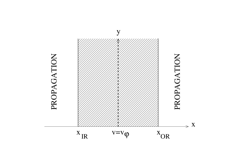
Figure 1: Wave propagation in a cartesian shear flow. Case where $dv/dx\neq 0$ and $B=0$: The shaded area indicate the regions where the waves are evanescent in the $x$–direction (they propagate only in the $y$–direction). $v_{\varphi}\equiv\omega/k_{y}$ is the phase velocity along the $y$–direction. The location $v=v_{\varphi}$ is not a singularity. Waves propagate in the $x$–direction beyond the turning points $x=x_{IR}$ and $x=x_{OR}$ given by equation (20).

In the limit $\left|v-v_{\varphi}\right|\gg c$, i.e. far enough from the turning points, the wavenumber in the $x$–direction, $k_{x}={\cal K}^{1/2}$, can be approximated by $k_{x}\simeq k_{y}\left|v-v_{\varphi}\right|/c\gg k_{y}$. This is characteristic of dispersive sound waves whose group velocity in the $x$–direction is $c$ and whose wavelength along $x$ decreases as they propagate outward. Again, this is equivalent to the density waves that propagate away from the Lindblad resonances in a Keplerian disc.

2.3.3 Case $dv/dx\neq 0$ and $B\neq 0$:

Here again we suppose $d^{2}v/dx^{2}=0$. As in the previous subsection, we have to solve equation (17) with ${\cal K}$ given by equation (18). It can be shown that:

$${\cal K}=\frac{k_{y}^{2}}{{\cal A}_{2}}\left[\frac{\left(v-v_{\varphi}\right)^{2}}{c^{2}}-1\right]^{-2}{\cal D},$$ (21)

where we have defined:

$${\cal D}\equiv-\frac{3}{k_{y}^{2}c^{2}}\left(\frac{dv}{dx}\right)^{2}+\left[\frac{\left(v-v_{\varphi}\right)^{2}}{c^{2}}-1\right]^{3}\left[1-\frac{1}{\beta}\frac{c^{2}}{\left(v-v_{\varphi}\right)^{2}}\right].$$ (22)

Then the condition ${\cal K}>0$ is equivalent to ${\cal A}_{2}{\cal D}>0$. We are going to study in turn the conditions ${\cal D}>0$ and ${\cal A}_{2}>0$.

We first suppose $\left|v-v_{\varphi}\right|/c\ll 1$. Then ${\cal D}>0$ is equivalent to:

$$\frac{\left(v-v_{\varphi}\right)^{2}}{c^{2}}<\frac{1}{\beta}\left[\frac{3}{k_{y}^{2}c^{2}}\left(\frac{dv}{dx}\right)^{2}+1\right]^{-1}.$$ (23)

If $\beta\gg 1$ (weak magnetic field) and/or $\left|dv/dx\right|\gg k_{y}c$, this condition is consistent with $\left|v-v_{\varphi}\right|/c\ll 1$. We note $x^{\prime}_{IR}$ and $x^{\prime}_{OR}$ the turning points corresponding to this condition.

We now suppose $\left|v-v_{\varphi}\right|/c$ is at least on the order of unity. Then, if $\beta\gg 1$ and/or $\left|v-v_{\varphi}\right|/c\gg 1$, ${\cal D}>0$ is equivalent to:

$$\frac{\left(v-v_{\varphi}\right)^{2}}{c^{2}}>\left[\frac{3}{k_{y}^{2}c^{2}}\left(\frac{dv}{dx}\right)^{2}\right]^{1/3}+1.$$ (24)

Again, this calculation is self-consistent if $\beta\gg 1$ and/or $\left|dv/dx\right|\gg k_{y}c$. Note that this condition is the same as that given by equation (20), so that the turning points are here again $x_{IR}$ and $x_{OR}$.

Finally, ${\cal A}_{2}>0$ is equivalent to:

$$\frac{\left(v-v_{\varphi}\right)^{2}}{c^{2}}>\frac{1}{\beta+1}.$$ (25)

Equation (17) has a (regular) singularity at $x=x_{IMR}$ and $x=x_{OMR}$ (where ’IMR’ and ’OMR’ stand for inner and outer magnetic resonances, respectively, by analogy with the magnetic resonances in a disc), where ${\cal A}_{2}=0$, i.e. $\left(v-v_{\varphi}\right)^{2}=c^{2}/\left(\beta+1\right)$. The flow however is well behaved at these locations, in contrast to the flow in a Keplerian disc (see T03). Note that in a Keplerian disc, the position of the magnetic resonances is given by exactly the same equation, provided $v_{\varphi}$ is replaced by the orbital velocity of the planet.

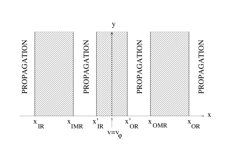
Figure 2: Same as figure 1 but for $B\neq 0$, and for the case $\beta\gg 1$ and/or $\left|dv/dx\right|\gg k_{y}c$. The turning points $(x^{\prime}_{IR},x^{\prime}_{OR})$, $(x_{IR},x_{OR})$ and $(x_{IMR},x_{OMR})$ are given by equations (23), (24) (or equivalently eq. [20]) and (25), respectively. Waves propagate in the $x$–direction beyond the turning points $x_{IR}$ and $x_{OR}$ but also in a restricted region around the magnetic resonances $x_{IMR}$ and $x_{OMR}$. The case represented here corresponds to $3\beta\left(dv/dx\right)^{2}>k_{y}^{2}c^{2}$. When this inequality is not satisfied, the points $(x^{\prime}_{IR},x^{\prime}_{OR})$ and $(x_{IMR},x_{OMR})$ have to be swapped.

In Figure 2, the shaded areas indicate where the waves are evanescent in the $x$–direction (the perturbation does propagate along the $y$–direction for all values of $x$), i.e. where ${\cal A}_{2}{\cal D}<0$. Waves propagate beyond the turning points that are also present in a non–magnetized disc, but they propagate as well in some restricted region around the magnetic resonances.

In the limit $\left|v-v_{\varphi}\right|\gg c$, i.e. far enough from the turning points $x_{IR}$ and $x_{OR}$, the wavenumber in the $x$–direction, $k_{x}={\cal K}^{1/2}$, can be approximated by:

$$k_{x}\simeq k_{y}\left(\frac{\beta}{\beta+1}\right)^{1/2}\frac{\left|v-v_{\varphi}\right|}{c}.$$ (26)

Note that, like in the non magnetic case, $k_{x}\gg k_{y}$ and the wavelength in the $x$–direction decreases as the waves propagate outward. This dispersion relation is characteristic of magneto–acoustic waves (fast mode) whose group velocity in the $x$–direction is $(c^{2}+v_{A}^{2})^{1/2}$. Again, this is equivalent to the waves that propagate away from the Lindblad resonances in a Keplerian disc (see eq. [37] and [38] in T03).

In the vicinity of the magnetic resonances, ${\cal A}_{2}\simeq 0$ and we can write ${\cal K}\simeq{\rm Const}/{\cal A}_{2}$. In the regions where ${\cal K}>0$, the wavenumber in the $x$–direction is $k_{x}={\cal K}^{1/2}$, so that the group velocity in this direction, $d\omega/dk_{x}$, can be calculated by using $2k_{k}dk_{x}/d\omega\simeq-({\rm Const}/{\cal A}_{2}^{2})d{\cal A}_{2}/d\omega$. This gives:

$$\frac{d\omega}{dk_{x}}\simeq{\cal A}_{2}^{3/2}\left[-\frac{3}{k_{y}c^{2}}\left(\frac{dv}{dx}\right)^{2}+\frac{v_{A}}{c}\left(\frac{c^{2}}{c^{2}+v_{A}^{2}}\right)^{3}\right]^{-1/2}\left(\frac{c^{2}}{c^{2}+v_{A}^{2}}\right)^{5/2}v_{A}.$$ (27)

This is characteristic of a slow MHD wave. Note that, as $d\omega/dk_{x}$ tends to zero as we approach the magnetic resonances, the waves propagate essentially along the magnetic field line in the vicinity of these resonances.

To summarize, fast magneto–acoustic waves propagate away from the Lindblad resonances while slow MHD wave propagates in the vicinity of the magnetic resonances. This situation is very similar to that in a Keplerian disc (T03), and these results are going to be used to interpret the numerical simulations that are presented below.

3 Numerical simulations

We perform numerical simulations of a low mass protoplanet embedded in a disc containing a toroidal magnetic field in order to study the properties of the magnetic resonances and in particular their effect on the migration of the planet.

3.1 Numerical setup

3.1.1 The method

We solved the MHD equations given in section 2.1 using a 2D adaptation of the 3D Eulerian code GLOBAL (Hawley & Stone 1995) and a modified version of NIRVANA (Ziegler & Yorke 1997). The algorithms used by both codes are very similar: they solve the above equations in cylindrical polar coordinates ($r$, $\phi$) using time-explicit finite differences. The magnetic field is evolved using the combined Method Of Characteristics and Constrained Transport (MOC-CT) algorithm which both preserves the divergence of the magnetic field and accurately describes the propagation of Alfvén waves (Hawley & Stone 1995).

Because the magnetic resonances lie very close to the orbit of the planet, a very high resolution is needed to resolve them. According to the linear theory, the distance between the planet and the magnetic resonances is (T03):

$$\mid r_{M}-r_{pl}\mid=\frac{2}{3}\frac{H}{\sqrt{1+\beta}}\,,$$ (28)

where $r_{M}$ and $r_{pl}$ are the radii of the magnetic resonances and of the planet, respectively, and $H$ is the disc semi–thickness. With the typical values of $H/r_{pl}=0.1$ and $\beta=2$ that we will use throughout this paper, we get $\mid r_{M}-r_{pl}\mid/r_{pl}=3.8\times 10^{-2}$. In order to accurately describe the magnetic resonances, we need to have roughly ten grid cells within this interval. On a uniform grid, when $r_{pl}=1$, this resolution would require about $550$ grid cells in the radial direction for a typical disc model whose radii range from $0.4$ to $2.5$. For such a resolution, each run would take months on a standard desktop computer. We have followed two routes to solve this problem. On the one hand, using GLOBAL, we built a non–uniform grid whose resolution increases in the neighborhood of the planet (see Appendix A for a detailed description of the grid setup). On the other hand, we ran NIRVANA on a multi-processor facility using the MPI library.

Using the first approach, we can run high resolution simulations with modest computational resources. However, the orbital radius of the planet has to be fixed so that it always remains in the high resolution part of the grid during the simulations. Note also that the calculation has to be made in the frame rotating with the planet, in which case the inertial forces are treated as described by Kley (1998). In the second case, we require access to powerful computing facilities, but the planet can move with respect to the grid, and we can study its actual migration in the disc. With the combination of both techniques, we have been able to analyze the effect of the magnetic resonances in detail.

3.1.2 The disc model

The disc parameters we used are described in detail in Nelson et al. (2000). We use dimensionless units for our numerical simulations. The unit of mass is taken to be the mass of the central star, $M_{\star}$=1, and the unit of length is taken to be the initial orbital radius of the protoplanet, $r_{pl}=1$. We set the gravitational constant $G=1$. We will consider a protoplanet with a mass $M_{pl}\ll M_{\star}$, so that, in a non self–gravitating disc, the unit of time can be approximated by $\left[r_{pl}^{3}/(GM_{\star})\right]^{1/2}$. The surface density is constant with radius, with $\Sigma=3\times 10^{-3}$. The inner boundary of the disc is located at $R_{in}=0.4$ and the outer boundary is at $R_{out}=2.5$. This results in quite a massive disc, and was chosen to give correspondingly rapid migration rates because of the long run times required by our high resolution simulations. In this paper, we only investigated the case $M_{pl}=1.5\times 10^{-5}$, which corresponds to $5$ Earth masses if the mass of the central star is that of the Sun.

The planet orbiting in the disc is modelled as a softened point mass. The total gravitational potential $\Phi$ that is exerted at any point of the disc is the sum of the potential of the central point mass and the potential of the planet:

$$\Phi(r,\phi)=-\frac{GM_{\star}}{r}-\frac{GM_{pl}}{\left[r^{2}+r_{pl}^{2}-2rr_{pl}\cos(\phi-\phi_{pl})+\epsilon^{2}\right]^{1/2}}+\frac{GM_{pl}}{r_{pl}^{3}}\;\mbox{\boldmath{$r$}}\mbox{\boldmath{$\cdot$}}\mbox{\boldmath{$r_{pl}$}}+\Phi_{ind}+\Phi_{disc}\,.$$ (29)

Here the planet is located at the point $(r_{pl},\phi_{pl})$. The parameter $\epsilon$ is the smoothing length of the gravitational potential. We took $\epsilon=0.1H$, so that it is smaller than the distance between the planet and the magnetic resonances. The third term in equation (29) is the indirect potential due to the planet, and accounts for the fact that the reference frame centered on the central star is non–inertial. The fourth term, $\Phi_{ind}$, represents the indirect potential due to the disc (see Nelson et al. 2000), and is non–zero only in simulations where the planet is allowed to migrate. The last term, $\Phi_{disc}$, corresponds to the potential due to the disc self–gravity, and is also non–zero only for simulations in which the planet migrates. In this work, we include only the axisymmetric component of the disc self–gravity, as we are concerned with accurately modelling the angular velocity of the disc gas and the embedded planet. Thus:

$$\Phi_{disc}(r)=-G\int_{R_{in}}^{R_{out}}\frac{{\overline{\Sigma}}(r^{\prime})\,r^{\prime}\,dr^{\prime}\,d\phi^{\prime}}{\sqrt{r^{2}+{r^{\prime}}^{2}-2rr^{\prime}\cos{(\phi-\phi^{\prime})}+\epsilon^{2}}}$$ (30)

where ${\overline{\Sigma}}(r)=\int\Sigma(r,\phi)d\phi/(2\pi)$. In this paper, we consider quite a massive disc model, as it produces more rapid migration rates. This means, however, that the disc gravity then makes a non–negligible contribution to the angular velocity of the disc material and embedded planet. The importance and effects of including $\Phi_{disc}$ are discussed further in section 3.3.

The equation of state is locally isothermal. The vertically integrated pressure $P=\Sigma c^{2}$ is calculated with the thin–disc approximation:

$$P=\left(\frac{H}{r}\right)^{2}\frac{GM_{\star}}{r}\;\Sigma\,.$$ (31)

The magnetic field is initially purely toroidal. Its strength is defined through the parameter $\beta$, which is the ratio of the square of the sound speed to the square of the Alfvén velocity at the initial location of the planet. A power–law variation of $B_{\phi}$ with radius is allowed:

$$B_{\phi}=\sqrt{\frac{\mu_{0}P(r=r_{pl})}{\beta}}\left(\frac{r}{r_{pl}}\right)^{-p}\,.$$ (32)

3.1.3 Boundary conditions

When we tried to use standard radial boundary conditions (outflow or reflecting, for example), we found that high frequency oscillations in the magnetic variables quickly started to grow. Eventually, in all of the cases we tested, these oscillations perturbed the entire disc to such an extent that no migration signal could be extracted. To overcome this problem we developed a damping procedure to reduce the amplitude of the waves generated by the planet as they approach the boundary.

Let $f$ be either components of the fluid velocity, and $f_{0}$ its equilibrium value. At the end of each timestep, we calculate a new value for $f$ according to the formula:

$$f=\left\{\begin{array}[]{ll}f_{0}+(f-f_{0})\times\exp\left[-\left(\frac{r-r_{i}}{\Delta_{i}}\right)^{2}\right]&\textrm{if $r<r_{i}$}\\ f&\textrm{if $r\in[r_{i},r_{o}]$}\\ f_{0}+(f-f_{0})\times\exp\left[-\left(\frac{r-r_{o}}{\Delta_{o}}\right)^{2}\right]&\textrm{if $r>r_{o}$}\end{array}\right.$$ (33)

We found that the best results were obtained when $r_{i}=0.55$ and $\Delta_{i}=0.35$, and $r_{o}=2$ and $\Delta_{o}=2$. It is crucial not to apply equation (33) to the magnetic field, because that would result in a violation of the constraint $\mbox{\boldmath$\nabla$}\mbox{\boldmath{$\cdot$}}\bf{B}=0$. Note that in the control hydrodynamic case that we did, this wave damping procedure produced almost the same torque on the planet as the standard reflective boundary conditions.

In cases when we used the logarithmic grid, we also found that more dissipation than just the standard artificial viscosity was required to reduce the level of high frequency noise. This dissipation was simply modelled by a small kinematic viscosity $\nu$ (see for example Nelson et al. 2000), which we took equal to $7.5\times 10^{-6}$. In our units, this is equivalent to adding an $\alpha$–viscosity (Shakura & Sunyaev 1973) with $\alpha=7.5\times 10^{-4}$. Over the time of our simulations, this small viscosity does not produce any significant change on the background disc structure. Its most important effect, as expected, is to broaden the magnetic resonances (see below). This viscosity was used in both the GLOBAL and NIRVANA runs.

3.1.4 Simulations properties

Model	$\beta$	$p$	resolution	grid type	migration
G1	$\infty$	-	$242\times 258$	VARIABLE	No
G2	2	0	$242\times 258$	VARIABLE	No
G3	2	0	$242\times 354$	VARIABLE	No
G4	2	0	$286\times 400$	VARIABLE	No
G5	2	1	$242\times 258$	VARIABLE	No
G6	2	2	$242\times 258$	VARIABLE	No
N1	2	0	$1000\times 1000$	UNIFORM	No
N2	2	0	$1000\times 1000$	UNIFORM	Yes
N3	2	1	$1000\times 1000$	UNIFORM	Yes
N4	2	2	$1000\times 1000$	UNIFORM	Yes

Table 1: Model parameters. Column $2$ gives $\beta=c^{2}/v_{A}^{2}$ at the initial location of the planet. Column $3$ gives $p$, the power-law exponent describing the variations of the magnetic field. Finally, columns $4$ and $5$ respectively give the resolution and type of the grid we used (uniform vs variable), while the last column indicates whether the planet is allowed to migrate or not.

The parameters of our runs are described in table 1. The first column gives their label. Its first letter indicates the code that has been used. “G” stands for models that have been run with GLOBAL, while models whose label starts with “N” have been performed with NIRVANA. Column 2 gives the ratio $\beta=c^{2}/v_{A}^{2}$ at the initial orbital radius of the protoplanet and column 3 gives the exponent $p$ of the magnetic field power law (see eq. [32]). Columns 4 and 5 describe the grid properties, giving the resolution and the type of the grid (uniform vs logarithmic). Finally, the last column states whether the planet is allowed to migrate through the disc or stay on a fixed orbit during its evolution. The initial coordinates of the planet are $(r_{pl},\phi_{pl})=(1,\pi)$. In the remaining of the paper, all times are measured in units of its initial orbital period $P=2\pi$.

3.2 Planet fixed on a circular orbit

In the simulations presented in this section, the planet is kept on a fixed circular orbit. The torque it exerts on the disc is computed, but the feedback torque from the disc on the planet is ignored.

3.2.1 Case of a uniform field

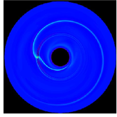
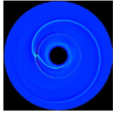
Figure 3: Disc surface density at time $t=5$ (left panel) and $t=10$ (right panel) in model G2. The slow MHD waves are seen propagating along the magnetic field lines, at the radius of the magnetic resonances.

We first begin with a description of our standard case, model G2. It starts with a uniform magnetic field in the disc, such that $\beta=2$ at the location of the planet. Using the logarithmic grid, the resolution in the neighborhood of the planet is $\Delta r=3\times 10^{-3}$, which gives about $12$ cells between the orbit of the planet and the predicted position of the magnetic resonances. We ran this model for $160$ orbits at the location of the planet.

When the simulation starts, the gravitational potential of the planet induces a perturbation on the disc. Fast magnetosonic waves, namely density waves modified by the magnetic pressure, are launched at the Lindblad resonances (defined as $x_{IR}$ and $x_{OR}$ in section 2.3.3) and propagate radially away from the planet orbit. Their behavior is very similar to that of density waves in the hydrodynamic case. Slow MHD waves also appear. They propagate azimuthally, along the magnetic field line, mostly at the expected location of the magnetic resonances (defined as $x_{IMR}$ and $x_{OMR}$ in section 2.3.3). This is illustrated by figure 3, which shows the surface density in the disc at times $t=5$ (left panel) and $t=10$ (right panel). The slow MHD waves are seen propagating around the disc. They are very tightly wrapped, indicating that they undergo very little radial propagation.

This is in complete agreement with the analysis presented in section 2.3.3 and the results displayed in figure 2. We have checked that in the simulations the waves that propagate around the magnetic resonances are dominated by values of $m$ in the range 0–5. In that case, the approximation $|dv/dx|\gg k_{y}c$ used in the analysis of section 2.3.3 is satisfied, and we are in the case displayed in figure 2 where the points $(x^{\prime}_{IR},x^{\prime}_{OR})$ are inside the magnetic resonances.

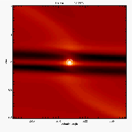
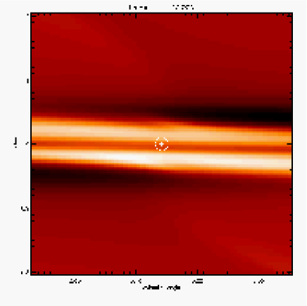
Figure 4: Snapshot of the density (left panel) and the toroidal component of the magnetic field $B_{\phi}$ (right panel) for model G2 after $120$ orbits. The white cross shows the position of the planet, while the radius of the circle is equal to the smoothing length. The magnetic resonances appear on both sides of the planet’s orbit as a decrease in the density and an increase in $B_{\phi}$.

The magnetic resonances appear very clearly on both sides of the planet’s orbit. This is shown in figure 4. The left panel represents the surface density in the vicinity of the planet at time $t=120$, while the right panel shows $B_{\phi}$. The magnetic resonances are apparent as a decrease in the density and an increase in the magnetic field. Note that this calculation is performed close to the linear regime. The perturbation of the variables is small compared to the equilibrium values. Indeed, the increase of the magnetic field strength is $18$% and the decrease of the density is only $4$%. This allows a close comparison between these simulations and the analytical results obtained in the linear regime (see section 2.3.3 and below). As noted above, the location of the magnetic resonances for $\beta=2$ is $r_{M}$ such that $|r_{M}-r_{pl}|/r_{pl}=3.8\times 10^{-2}$. This agrees with figure 4, from which we can also see that the perturbation is much more important inside these resonances than outside. This suggests that the turning points $x^{\prime}_{IR}$ and $x^{\prime}_{OR}$ defined in section 2.3.3 are inside the resonances, i.e. waves propagate in a restricted region inside the resonances, as illustrated in figure 2.

An important goal of these simulations is to investigate the effect of the magnetic resonances on the torque exerted by the disc on the planet. The torque ${\bf T}_{pl}$ exterted by the planet on the disc is:

$${\bf T}_{pl}=-\int\!\!\!\int_{disc}\Sigma{\bf r}\mbox{\boldmath$\times$}\frac{GM_{pl}\left({\bf r}-{\bf r_{pl}}\right)}{\mid{\bf r}-{\bf r_{pl}}\mid^{3}}\,r\,\textrm{d}r\,\textrm{d}\phi$$ (34)

The torque ${\bf T}$ exerted by the disc on the planet is $-{\bf T}_{pl}$. Its value, normalized by the quantity $GM_{pl}r_{pl}$, is:

$$T=\int\!\!\!\int_{disc}\frac{\Sigma r^{2}\sin(\phi-\phi_{pl})\,\textrm{d}r\,\textrm{d}\phi}{\mid{\bf r}-{\bf r_{pl}}\mid^{3}}\;.$$ (35)

Figure 5 shows the time history of $T$ for model G2: the upper curve plots the torque exerted on the planet by the inner part of the disc ($r<r_{pl}$). It is positive, which indicates that the inner disc tends to produce outward migration. The lower curve shows the torque exerted by the outer disc ($r>r_{pl}$) on the planet. The middle curve is the sum of the two, i.e. the total torque exerted by the disc on the planet. One can see that it saturates at a constant and negative value after $80$ orbits. Note also the high frequency variations appearing at the end of the simulation (for $t>140$). They are due to our particular treatment of the inner boundary condition. However, they do not influence the overall behavior of the disc. As in the hydrodynamic case, figure 5 demonstrates that the disc causes the planet to migrate inward. This is because the inner and outer magnetic resonances balance each other in that case.

Figure 5: Time history of the torque exerted by the disc on the planet for model G2. From bottom to top, the curves respectively show the outer torque, the total torque and the inner torque. Since the total torque is negative, the planet migrates inward.

Figure 6: Torque exerted on the planet by the annulus with radii between $r_{pl}$ and $r$ as a function of $|r-r_{pl}|/r_{pl}$ for model G2. The solid line shows $T(r<r_{pl})$ and the dashed line $-T(r>r_{pl})$. The magnetic resonances are obvious at $|r-r_{pl}|/r_{pl}\simeq 0.03$. The expected value from linear theory is $0.038$.

Nevertheless, both resonances still affect the torque, as is illustrated in figure 6. The dashed line shows the quantity $-T(r>r_{pl})$, which is the opposite of the torque exerted on the planet by an annulus with radii between $r_{pl}$ and $r>r_{pl}$ as a function of $|r-r_{pl}|/r_{pl}$ for model G2. The solid line shows the inner torque $T(r<r_{pl})$. On both curves, the magnetic resonances show up as a peak in these quantities. Their radii is around 0.03. This is in reasonable agreement with linear theory, which gives $\mid r-r_{M}\mid=0.038$ for the parameters of model G2. Note that their width is larger than expected in an invicid disc because of the $\alpha$–type viscosity used here. This is probably why they are not exaclty at 0.038. Runs performed in an inviscid disc for a shorter period indeed show the resonances at their expected radii (Fromang 2004).

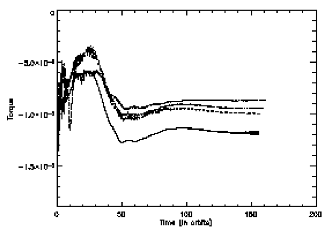
Figure 7: Comparison of the total torque exerted by the disc on the planet for model G2 (solid line), G3 (dashed line), G4 (dotted line) and N1 (dotted-dashed line). In all cases, the saturated torques lie between $-8.5\times 10^{-6}$ and $-1.2\times 10^{-5}$. This indicates that the results presented in this paper only weakly depend on the code and on the resolution.

In figure 7 we plot the torque corresponding to a variety of simulations performed with differing resolutions. Results from runs G2, G3, and G4 are plotted here, showing modest dependence of the torque on resolution.

Also plotted in figure 7 are the torques calculated from run N1 performed using NIRVANA. Here a uniform grid in $r$ and $\phi$ was used, with ($N_{r}$, $N_{\phi}$)=(1000, 1000) grid cells being employed. This gives a resolution of $\Delta r=2.1\times 10^{-3}$, so that there are $\sim 18$ grid cells between the location of the planet and the predicted location of the magnetic resonances. The model was run with the planet being held on a fixed circular orbit, in a rotating frame that corotates with the planet, for a time of 160 orbits. The resulting torques are in very good agreement with those obtained during runs G2 , G3 and G4.

3.2.2 Case of a non–uniform field

In this section, we investigate the effect of a radial gradient of the magnetic field on the migration properties of the protoplanet. To do so, we ran $3$ MHD simulations, models G2 (described above), G5 and G6, corresponding to $p=0,1,2$ respectively (see eq. [32]). All of the other parameters of the three simulations are the same. We also compare these models with model G1, a case without a magnetic field ($B_{\phi}=0$).

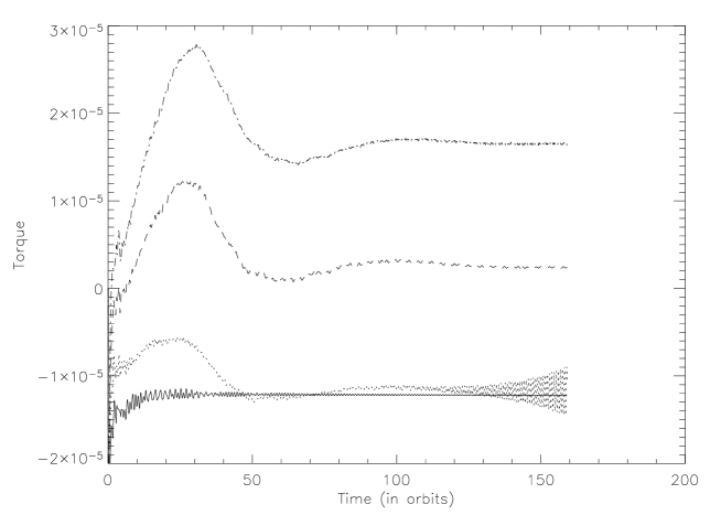
Figure 8: Total torque $T$ exerted by the disc on the planet for model G1 (solid line), G2 (dotted line), G5 (dashed line) and G6 (dotted–dashed line). $T$ increases as the magnetic field steepens and becomes positive when $B_{\phi}\propto r^{-2}$: the planet will migrate outward in that case.

Figure 9: Radial profile of the toroidal component of the magnetic field at the azimuth of the planet for model G2 (solid line), G5 (dotted line) and G6 (dashed line).

For each of these models, the time history of the total torque exerted by the disc on the planet is plotted in figure 8. The solid curve corresponds to model G1, while the other curves are deduced from model G2 (dotted line), G5 (dashed line) and G6 (dotted–dashed line). All of them were run for $160$ orbits, a long enough time to reach saturation, which occurs between $80$ and $90$ orbits. The total torques obtained in models G1 and G2 are very close. This is because the effects of the magnetic resonances located on both sides of the orbit of the planet cancel each other in G2. The hydrodynamic result is recovered in that case. However, there is a clear tendency for the torque to increase (ie becoming less negative/more positive) when the magnetic field becomes steeper. As was already described above, it is negative for model G2. For model G5, it is almost equal to zero, indicating that the migration of the planet should be very slow in that case. Finally, for model G6, it is positive. The planet should show strong outward migration. This trend can be qualitatively understood with the help of figure 9, where the radial profile of $B_{\phi}$ at the azimuth of the planet is plotted for model G2 (solid line), G5 (dotted line) and G6 (dashed line). As the magnetic field gets steeper, the inner magnetic resonance gets stronger and the outer magnetic resonance gets weaker. The balance between the positive torque exerted in the neighborhood of the inner magnetic resonance and the negative torque exerted near the outer magnetic resonance is biased in favor of the former and the net torque increases.

We now compare these values of the torque with the values computed from the linear analysis (see T03). To recover SI units, the torques given above have to be multiplied by $GM_{pl}M_{\star}/r_{p}$. This gives $T=-3.2\times 10^{29}$, $5.34\times 10^{28}$ and $4.5\times 10^{29}$ SI for $p=0,1$ and 2, respectively. The linear analysis gives $T=-5.06\times 10^{29}$, $-1.01\times 10^{29}$ and $3.7\times 10^{29}$ SI for $p=0,1$ and 2, respectively. The agreement for $p=0$ and $p=2$ is very good, the difference between the torques being 37 and 21%, respectively. The agreement is not as good for $p=1$, but note that in that case the torque is small, which makes it more difficult to get a good accuracy from the simulations. The torque obtained from linear theory in the case $B=0$ is $-5.04\times 10^{29}$ SI, very close to the torque corresponding to $p=0$. This also agrees very well with the numerical simulations.

3.3 Migrating planets

In addition to performing simulations in which the planet is held on a fixed circular orbit, runs were performed to investigate the actual migration of the planet as a function of the magnetic field profile in the disc. These runs are listed as N2, N3 and N4 in table 1.

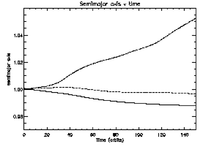
Figure 10: Time evolution of the semimajor axes for simulations N2 (solid line), N3 (dashed line) and N4 (dashed-dotted line). While simulations N2 and N3 lead to inward migration, simulation N4, with the larger magnetic field gradient, leads to outward migration.

The variation of semimajor axis with time is shown in figure 10 for these three runs. Run N2 is shown by the solid line, N3 by the dashed line, and N4 by the dotted-dashed line. These calculations are in basic agreement with their GLOBAL counterparts, and analytic expectations, in that they display quite rapid inward migration (N2 and G2), slow migration (N3 and G5), and strong outward migration (N4 and G6). These latter simulations provide definitive evidence that a strong radial gradient in magnetic field in an accretion disc can stop and even reverse type I migration.

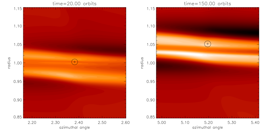
Figure 11: The left panel shows a contour plot of $r^{2}B_{\phi}$ for run N4 at $t=20$. The right panel shows a similar plot at time $t=150$. The locations of the magnetic resonances are seen to track the radial location of the planet (shown by the black cross) as it migrates outward.

In figure 11 we present contour plots of $B_{\phi}$ in the vicinity of the planet for run N4 at $t=20$ and $150$ orbits. The left hand panel shows the magnetic resonances being established near the beginning of the simulation. The right panel shows the field strength to have increased at the resonances after 150 orbits, and also shows the resonant locations tracking the radial position of the planet as it migrates outward. We note that the planet position (shown by a black cross) appears to be closer to the outer magnetic resonance than the inner one at this time. We speculate that this may be due to the readjustment time of the disc being comparable to the migration time in this run. Indeed, the disc response time is about 70–80 orbits, as shown by figure 5, which is the time required for the torques to approach steady values, and for the magnetic field to achieve an approximate steady state at the magnetic resonances.

In section 3.1.2 we discussed briefly the inclusion of the axisymmetric component of self–gravity in our simulations of migrating planets. Normally the disc mass used in simulations of the type presented here is sufficiently small that this is not required. However, because the simulations here are of high resolution, and therefore computationally expensive, we are compelled to use a fairly massive disc with correspondingly faster migration rates. Not including the disc self–gravity, but including the acceleration by the disc on the planet’s orbital evolution, has the effect of increasing the inward radial force experienced by the planet, thus increasing its angular velocity. This causes a shift in the angular frequency associated with the planet’s orbital motion that modifies slightly the positions of the Lindblad and magnetic resonances, making the outer resonances stronger relative to the inner ones. Including the disc self–gravity helps to remove this effect. Given the close proximity of the magnetic resonances to the planet orbital radius, we have found that such shifts in frequency can qualitatively change results. For example, we ran a case similar to run N4, but without the disc self–gravity, and found the outward migration stalled after $t<100$ orbits. Including the self–gravity removes this stalling effect.

4 Discussion

We have performed numerical simulations of a low–mass planet embedded in a disc containing a toroidal magnetic field using two different codes. In the runs performed with GLOBAL, the grid was logarithmic and the planet was kept on a fixed circular orbit. By contrast, in the runs performed with NIRVANA, the grid was uniform and the planet was allowed to migrate under the effect of the torque exerted by the disc.

An important aspect of these simulations was to study the effect of the magnetic resonances on the migration of the planet. Since these resonances are located very close to the planet’s orbit, at only a fraction of the disc semi–thickness, a very high resolution was required.

In agreement with the linear theory, we have found that magneto–acoustic waves propagate radially away from the planet beyond the Lindblad resonances, whereas slow–MHD waves propagate essentially along the field lines at the location of the magnetic resonances. For the parameters we adopted in this paper, the torque exerted by the region of the disc around these resonances tended to dominate the Lindblad torque. We found inward and outward migration for a uniform field and for a field varying as $r^{-2}$, respectively. The torques computed from the simulations were in very good agreement with those calculated from the linear theory. For a field varying like $r^{-1}$, we found outward migration with GLOBAL and inward migration with NIRVANA, in both cases at a rate much reduced compared to when the field is uniform. The linear theory predicted inward migration in that case, also at a reduced rate. This shows that the simulations performed here are at the limit of what can be achieved today.

These simulations confirm that, if the magnetic field has a gradient which is locally steep enough, migration of low–mass planets can be reversed.

An interesting feature that was seen in the simulations is that, if the adjustement time of the disc (and therefore of the resonances) is comparable or longer than the migration time, which may be the case for a massive disc, then the position of the planet with respect to the resonances is affected. In the case $p=2$, the planet, which was migrating outward, got closer to the outer resonance. We may then expect the migration to be slowed down, as the outer resonance becomes more important, until the disc readjusts. By contrast, for a planet migrating inward, the inner resonance would get closer and in that case again migration would slow down.

Note that the slow MHD waves that propagate around the magnetic resonances are the modes which are destabilized in the magnetorotational instability (Balbus and Hawley 1991). Therefore, it is not clear that the processes that are described here would still operate if the field were weak enough to be unstable. Note however that the modes that are magnetorotationally unstable have large values of $m$ (Balbus and Hawley 1992, Terquem and Papaloizou 1996), whereas the modes that are important here have low values of $m$. So it is possible that the resonances described here still operate to reverse planet migration in an unstable disc, i.e. in the presence of turbulence.

In the simulations presented in this paper, as in the analysis of T03, the disc is assumed to be infinitessimally thin. As the distance between the planet and the resonances involved in the disc/planet interactions is smaller than the disc semithickness, this approximation is actually not valid. However, in the absence of a magnetic field, results from 3D calculations were not found to be qualitatively different from those from 2D calculations. This is because the total Lindblad and corotation torques of 3D waves (with vertical motions) are much smaller than those of 2D waves. So the only effect of the 2D approximation is to introduce a vertical averaging of the gravitational potential of the protoplanet. This results in the Lindblad and corotation torques being 60% and 50% larger, respectively, in 2D than in 3D (Tanaka et al. 2002). In the case of a magnetized disc, we anticipate that the torque from the magnetic resonances will be similarly reduced in 3D.

It is the angular momentum carried by the perturbation in the vicinity of the magnetic resonances which enables the planet to reverse its migration. When there is no magnetic field, the angular momentum carried by the density waves beyond the Lindblad resonances is carried away from the planet. The waves that propagate around the magnetic resonances are trapped there though. So it is not clear how the angular momentum they carry is transported away. If the waves were just bouncing back and forth in some finite region, there would be no net exchange of angular momentum between the planet’s orbital motion and the disc’s rotation. Therefore, it is possible that the modes that propagate around the magnetic resonances tunnel through the region where the disc response is evanescent. The detail of the processes by which angular momentum is exchanged will be the subject of a future paper.

Appendix A The logarithmic grid

In this appendix, we describe in detail the logarithmic grid that was used for model G1 to G6. Its aim is to increase the resolution in the neighborhood of the planet with a low cost on the computing time.

The radial grid is composed of three zones: first, a buffer zone, $r\in[Rb1,Rb2]$, where each cell has the same size, encompasses the orbit of the planet. In the region $[R_{in},Rb1]$, the resolution increases has $r$ increases: $(\Delta r)_{i}/(\Delta r)_{i+1}=h$. This is the opposite in the region $[Rb2,R_{out}]$. There, again, the size of the cells increases as one goes away from the planet.

The azimuthal grid has similar properties. Since the planet is located at $\phi_{pl}=\pi$, there is a buffer zone, with constant grid spacing, in the interval $\phi\in[\pi-\pi/20,\pi+\pi/20]$. On both sides of this zone, the size of the grid cells is increasing with the same ratio $h$ as for the radial grid.

Figure 12 illustrates the resulting grid topology. The planet is located in the shaded grid zone, where the resolution is the highest. Note that the ratio between neighboring cells sizes has been exaggerated for clarity in this figure. For the actual simulations presented in this paper, we used $Rb1=0.9$, $Rb2=1.1$ and $h=1.02$. For our fiducial run, model G2, we used $60$ cells in the buffer zone of the radial grid, which gives a resolution $\Delta r=3.3\times 10^{-3}$. The cell size in $\phi$, which is not so crucial for a good description of the magnetic resonances, was taken to be twice this value at the location of the planet: $r_{pl}\Delta\phi=6.6\times 10^{-3}$. On a uniform grid, the number of cells required to reach such a resolution would have been $N_{r}=630$ and $N_{\phi}=950$. Here, with the help of the logarithmic grid, the actual resolution is $(N_{r},N_{\phi})=(242,258)$. For model G3, the number of cells in the buffer zone was doubled in the azimuthal direction, while for model G4 it was composed of $80$ cells in both directions.

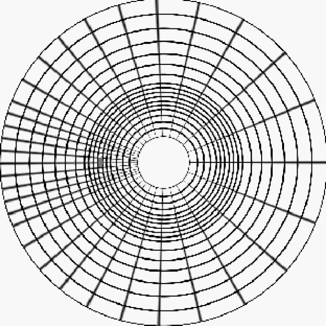
Figure 12: Cartoon illustrating the properties of the grid. The position of the planet is shown by the grey area. The resolution is higher there than what it is elsewhere in the computational domain. Note that the ratio between neighboring cells sizes has been exaggerated here for clarity.

References

- [1991] Balbus S. A., & Hawley J. F., 1991, ApJ, 376, 214
- [1992] Balbus S. A., & Hawley J. F., 1992, ApJ, 400, 610
- [1998] Balbus S. A., & Hawley J. F., 1998, Rev. Mod. Phys., 70, 1
- [1998] Boss A. P., 1998, ApJ, 503, 923
- [2004] Fromang S., 2004, PhD Thesis
- [1979] Goldreich P., & Tremaine S., 1979, ApJ, 233, 857 (GT79)
- [1995] Hawley J. F., Stone J. M., 1995, Comput. Phys. Commun., 1995, 89, 127
- [2003] Lecar M., Sasselov D. D., 2003, ApJ, 596, 99
- [1993] Lin D. N. C., & Papaloizou J. C. B., 1993, in Protostars and Planets III, eds. E. H. Levy, & J. I. Lunine (Tucson: University of Arizona Press), p. 749
- [2003] Matsuyama I., Johnstone D., Murray, N., 2003, ApJ, 585, 143
- [2000] Nelson, R. P., Papaloizou J. C. B., Masset F., Kley W., 2000, MNRAS, 318, 18
- [2004] Nelson, R. P., Papaloizou J. C. B., 2004, MNRAS, 350, 849
- [1996] Pollack J.B., Hubickyj O., Bodenheimer P.; Lissauer J. J., Podolak M., Greenzweig Y., 1996, Icarus, 124, 62
- [2002] Tanaka H., Takeuchi T. & Ward W. R., 2002, ApJ, 565, 1257
- [1996] Terquem C., & Papaloizou J. C. B., 1996, MNRAS, 279, 767
- [2003] Terquem C., 2003, MNRAS, 341, 1157 (T03)
- [1998] Trilling D. E., Benz W., Guillot T., Lunine J. I., Hubbard W. B., Burrows A., 1998, ApJ, 500, 428
- [2003] Udry S., Mayor M. & Santos N. C., 2003, A&A, 407, 369
- [1986] Ward W. R., 1986, Icarus, 67, 164
- [1997] Ward W. R., 1997, Icarus, 126, 261
- [1997] Ziegler U., Yorke H. W., 1997, Comput. Phys. Commun., 101, 54