Black Hole Masses and Eddington Ratios at $0.3<z<4$

Abstract

We study the distribution of Eddington luminosity ratios, $L_{\rm bol}/L_{\rm Edd}$, of active galactic nuclei (AGNs) discovered in the AGN and Galaxy Evolution Survey (AGES). We combine H$\beta$, Mg II, and C IV line widths with continuum luminosities to estimate black hole (BH) masses in 407 AGNs, covering the redshift range $z\sim 0.3-4$ and the bolometric luminosity range $L_{\rm bol}\sim 10^{45}-10^{47}$ erg s^-1. The sample consists of X-ray or mid-infrared (24$\micron$) point sources with optical magnitude $R\leq 21.5$ mag and optical emission line spectra characteristic of AGNs. For the range of luminosity and redshift probed by AGES, the distribution of estimated Eddington ratios is well described as log-normal with a peak at $L_{\rm bol}/L_{\rm Edd}\simeq$ 1/4 and a dispersion of 0.3 dex. Since additional sources of scatter are minimal, this dispersion must account for contributions from the scatter between estimated and true BH mass and the scatter between estimated and true bolometric luminosity. Therefore, we conclude that: (1) neither of these sources of error can contribute more than $\sim$0.3 dex rms; and (2) the true Eddington ratios of optically luminous AGNs are even more sharply peaked. Because the mass estimation errors must be smaller than $\sim$0.3 dex, we can also investigate the distribution of Eddington ratios at fixed BH mass. We show for the first time that the distribution of Eddington ratios at fixed BH mass is peaked, and that the dearth of AGNs at a factor $\sim 10$ below Eddington is real and not an artifact of sample selection. These results provide strong evidence that supermassive BHs gain most of their mass while radiating close to the Eddington limit, and they suggest that the fueling rates in luminous AGNs are ultimately determined by BH self-regulation of the accretion flow rather than galactic scale dynamical disturbances.

1 Introduction

For well over 30 years, the basic theory of active galactic nuclei (AGNs) has been that they are luminous because of the accretion of matter onto black holes (BHs; Salpeter 1964; Zel’dovich & Novikov 1964; Lynden-Bell 1969). In this picture, the luminosity produced by a BH of mass $M_{\rm BH}$ has a natural maximum, the Eddington limit ($L_{{\rm Edd}}$), at which the radiation pressure due to the accretion of the infalling matter balances the gravitational attraction of the BH. Most models for AGNs assume that they are BHs radiating near the Eddington limit, and as techniques for independently estimating BH masses in AGNs have been developed, it has become possible to test this supposition. In particular, large, modern spectroscopic surveys can provide estimates of the Eddington ratios (the ratio of the AGN bolometric luminosity to the Eddington limit) for thousands of AGNs (see, e.g., analyses of the Sloan Digital Sky Survey [SDSS] by McLure & Dunlop [2004] and M. Vestergaard et al., in preparation). Unfortunately, the shallowness of these large, wide-area surveys imposes severe restrictions on the combinations of Eddington ratio and BH mass that are observable, especially at $z>1$. For $M_{\rm BH}\lesssim 10^{9}M_{\odot}$, the SDSS is sensitive only to near-Eddington radiators above this redshift, and even at $z<1$ the SDSS analyses to date have not clearly established whether there is a lower cutoff to the $L_{\rm bol}/L_{\rm Edd}$ distribution at fixed BH mass. Warner et al. (2004) derived BH masses for over 500 ($0\leq z\leq 5$) AGNs and found a broad range of Eddington ratios. However, it is difficult to draw any conclusions about the underlying distribution of $L_{{\rm bol}}/L_{{\rm Edd}}$ because their dataset is heavily weighted toward high-luminosity objects.

The AGN and Galaxy Evolution Survey (AGES; Kochanek et al., 2004) probes nearly a decade further down the AGN luminosity function than the SDSS. For the first time, this permits a relatively unbiased measurement of the distribution of Eddington ratios at fixed BH mass at $z\geq 1$, while the distribution at fixed luminosity can be measured down to $z=0.5$. The AGES survey uses the 300-fiber Hectospec robotic spectrograph on the MMT (Fabricant et al., 1998; Roll et al., 1998; Fabricant et al., 2005) to survey galaxies and AGNs in the Boötes field of the NOAO Deep Wide-Field Survey (NDWFS; Jannuzi & Dey, 1999). Both a population of high mass BHs radiating significantly below Eddington and a population of low mass BHs radiating near or above Eddington would be observable with AGES. In this paper we show: (1) that the distribution of Eddington ratios at fixed BH mass or at fixed luminosity is narrowly peaked and well-described by a single log-normal distribution independent of redshift and luminosity, (2) that this peak occurs at roughly 1/4 of the Eddington limit, and (3) that the rms error in BH mass estimates from emission-line scaling relations is less than $\sim$0.3 dex at fixed luminosity. The first two conclusions imply that the luminous growth of BHs over cosmic time is dominated by objects radiating near the Eddington limit.

We present a brief overview of our data from the AGES survey in § 2 and describe our method of analysis in § 3. We present our BH mass estimates and Eddington ratios as functions of redshift and luminosity in § 4. Finally, we discuss the implications of these results in § 5. In our analysis, we assume an $H_{0}=72\;{\rm km\;s^{-1}}\;{\rm Mpc^{-1}},\Omega_{m}=0.3,\Omega_{\Lambda}=0.7$, flat cosmology.

2 Data

AGES is a redshift survey in the roughly 9 deg² Boötes Field that had been imaged by the NDWFS in $B_{\rm W}$, $R$, and $I$ filters. Subsequent surveys have imaged the field at many wavelengths, providing a rich multi-wavelength data set. In this paper, we make particular use of data from the Chandra X-ray Observatory XBoötes survey (Murray et al., 2005; Brand et al., 2006; Kenter et al., 2005), and the Spitzer Space Telescope (MIPS: Rieke et al. 2004; IRAC: Eisenhardt et al. 2004).

The AGES-I Survey (C. Kochanek et al., in preparation) selected AGN candidates as either X-ray or 24$\micron$ sources, with $R\leq 21.5$ mag (Vega) optical point source counterparts. Objects were considered to be point sources, if they were point-like in any one of $R$, $I$, or $B_{\rm W}$. Since the luminosities we consider here are higher than the canonical Seyfert luminosities, there should be little contribution from host galaxies in these AGNs. The primary sample of $z>1$ AGNs consists of either XBoötes sources with $\geq 4$ counts (over an average exposure time of 5 ks) or 24$\micron$ sources brighter than 1 mJy that are off the stellar locus (2MASS $J>[12+2.5\;{\rm log}F_{24\mu{\rm m}}]$). These are supplemented by X-ray sources with 2 or 3 counts and 24$\micron$ sources with $0.5~{}{\rm mJy}<F_{24\mu{\rm m}}<1~{}{\rm mJy}$. Redshifts were obtained with Hectospec at the MMTO. The spectra were analyzed by two independent pipelines and verified by eye. This led to a sample of 733 broad-line AGNs with $z>0.1$. We analyze a subset of this sample for which we can reliably measure emission line widths, as described in §3.1.

2.1 Completeness

There are three issues for understanding the completeness of our sample: the literal completeness of the spectroscopy, the effects of the optical flux limits, and the effects of the 24$\micron$/X-ray flux limits. The first, the completeness of the spectroscopy, plays no role in our conclusions. While we did not obtain spectra of every candidate matching our selection criteria, we did obtain redshifts for 97% of the candidates for which we obtained spectra. These represented only 66% of the candidates, but the candidates with spectra can be regarded as a “random” sub-sample of the candidates that was dictated by the fraction of the NDWFS region covered by spectroscopy and whether it was possible to assign fibers to the candidates. Presumably neither of these issues are correlated with either Eddington ratio or BH mass. Thus, the only question is whether the spectrum allowed the measurement of the line FWHM, and we discuss this in § 3.1. The second issue, the optical flux limit imposed for the spectroscopic targets, we will include explicitly in our analysis.

It is the third issue, the consequences of the 24$\micron$ and X-ray flux limits that we must consider in more detail. Our X-ray limit is the deepest in the survey (see Brand et al., 2006), and therefore no correction is necessary for the X-ray completeness. However, if we examine the distribution of AGNs in the plane of the $R$-band and 24$\micron$ fluxes, it is clear that both of these flux limits matter. Our spectroscopic limit is nominally defined by $R=21.5$ mag. However, the 24$\micron$+X-ray selected sample is only complete to $R=19.1$ mag. We evaluate the problem and estimate a correction by using the deeper samples from the AGES-II catalogs (C. Kochanek et al., in preparation). AGES-II includes AGNs selected using mid-infrared colors from the IRAC Shallow Survey (Eisenhardt et al., 2004), based on the color selection method outlined in Stern et al. (2005), as well as the 24$\micron$ and X-ray criteria used for AGES-I. This leads to an AGN sample with a 3.6$\micron$ (approximately $L$-band) flux limit of $[3.6]=18$ mag and an optical limit of $I=21.5$ mag that fills in most of the missing quasars to the optical flux limit of AGES-I. The AGES-II $[3.6]=18$ mag limit, combined with the fact that $z>1$ AGNs have $R-[3.6]>2.9$, implies that the survey is complete to $R=20.9$ mag. Brighter than this magnitude, we simply compare the AGES-I and AGES-II samples to determine the required completeness correction. For fainter AGNs, we must apply an additional correction that incorporates the fraction of AGNs that are lost in AGES-II owing to their relatively blue colors with respect to the [3.6] limit. This correction factor is known from the brighter magnitudes where AGES-II is complete. We show the functional form for our completeness correction in Figure 1.

These corrections for completeness are important for the interpretation of the results in §4.2, and we return to the completeness corrections and how they affect our conclusions there.

3 Analysis

BH masses have been estimated from H$\beta$ emission line widths and luminosities for some time (e.g., Dibai, 1980). However, it was only with the application of reverberation mapping (for an overview, see Peterson, 2001) that this relationship became firmly established, and then was revised with improved data and techniques (Kaspi et al., 1996; Wandel, Peterson & Malkan, 1999; Kaspi et al., 2000; McLure & Jarvis, 2002; Vestergaard, 2002; Kaspi et al., 2005; Vestergaard & Peterson, 2006; Bentz et al., 2006). The general form of the relation is:

$$\log M_{\rm BH}=a+b\log(\lambda L_{44})+2\log V,$$ (1)

where $M_{\rm BH}$ is the estimated BH mass in units of M_⊙, $V$ is the H$\beta$ full width at half maximum (FWHM) in ${\rm km\;s^{-1}}$, and $\lambda L_{44}$ is the continuum luminosity near the line (5100 Å) in units of 10${}^{44}\;{\rm erg\;s^{-1}}$. Because optical spectra can only probe H$\beta$ to a maximum redshift of $z\sim 0.75$, studies have been undertaken to find scaling relationships for UV lines, allowing the estimation of black hole masses at high redshift. A relationship for C IV $\lambda$1549 and the 1350 Å continuum (probing $1.6\leq z\leq 5$) was calibrated from reverberation-based H$\beta$ measurements and single-epoch C IV observations (Vestergaard, 2002), which is well-matched to the luminosity range probed by AGES-I. For intermediate redshifts ($0.4<z<2$), McLure & Jarvis (2002) determined a scaling relationship for Mg II $\lambda$2800 by comparing single-epoch measurements of Mg II FWHM and 3000 Å continuum luminosity with results from H$\beta$ reverberation mapping under the assumption that the two lines are emitted at the same distance from the BH due to their similar ionization potentials. While the response of Mg II in reverberation mapping campaigns has been rather weak (see Clavel et al. 1991 and Dietrich & Kollatschny 1995 for the best result, that of NGC 5548), reverberation studies of C IV have yielded BH masses in good agreement with those from H$\beta$ (e.g., Onken & Peterson, 2002). There has been a long struggle to measure BH masses from these emission lines and each line has associated peculiarities. We refer the reader to the original works, which address these issues in greater detail.

We adopt ($a,~{}b$)=(0.68, 0.61) in equation (1) for the H$\beta$ relation (from McLure & Jarvis, 2002, although other versions of the relation differ by less than $\approx$0.10 in slope); we use ($a,~{}b$)$=$(0.20, 0.7) for C IV (from Vestergaard, 2002); and we estimate in § 3.3 that ($a,~{}b$)$=$(0.31, 0.88) for Mg II. We measure the line widths from the AGES-I spectra (§ 3.1) and the continuum luminosity from the NDWFS photometry (§ 3.2). We discuss the sensitivity of our results to the exact parameters of these relations in § 4.3.

3.1 Line Width

The AGES-I spectra have a pixel scale of 1.2 Å and a resolution of $\approx 6$ Å FWHM. For our analysis, we boxcar-smooth the spectra over 11 pixels, then subtract a locally-defined linear continuum from the region around the emission line of interest. The rest-frame wavelength regions used to set the continuum around each line are (4740-4765 Å, 5075-5100 Å) for H$\beta$, (2670-2682 Å, 2940-2970 Å) for Mg II, and (1455-1465 Å, 1700-1705 Å) for C IV. We subtract narrow-line contributions to H$\beta$ using the [O III] $\lambda$5007 line as a model, with the [O III] flux scaled by a factor of 0.15. This fiducial value for the (narrow H$\beta$)-to-[O III] flux ratio lies within the range defined by local AGNs that have only narrow emission lines (Baldwin et al. 1981; Veilleux & Osterbrock 1987). Visual inspection of the post-subtraction spectra revealed little residual narrow-line contribution. We determine the peak flux in the line region and measure the FWHM of the line as follows (adapted from Peterson et al., 2004, and illustrated in Fig. 2). First, we determine two wavelengths on each side of the line: (1) the first crossing of the half-max flux level moving downward from the line peak (indicated as Blue1 and Red1 in Fig. 2); (2) the first half-max crossing moving upward from the line edge (Blue2 and Red2). The mean of these two wavelengths is taken as the half-max point for that side of the line (Blue and Red). The FWHM is defined as the difference between the Blue and Red points. The boxcar smoothing of 13 Å serves to minimize the sensitivity of our automated procedure to noise in the spectra and results in a final resolution of $\sim 500~{}{\rm km\;s^{-1}}$. This adds a negligible ($\sim$2%) systematic contribution to our measured FWHM, for which we do not correct. We estimate the error in the FWHM with the technique described by Corbett et al. (2003), in which line gradients at the half-max points are used to convert the Poisson noise of the spectral counts at half-max into wavelength uncertainties. A minimum FWHM error of 10% is imposed on all measurements.

To remove spurious measurements from the dataset, every spectrum is examined for a series of problems: anomalous features (e.g., sky subtraction artifacts), significant absorption in the line profile, strong Fe II emission around Mg II, and low signal-to-noise ratio (S/N). The presence of broad absorption in AGNs has been found to be independent of Eddington ratio (Scoggins et al. 2004), so the lines removed for strong absorption (mainly C IV) should be unbiased with respect to Eddington ratio. In addition, the Eddington ratio distributions we observe for objects with masses from Mg II and from C IV are similar, despite Fe II contamination being much less significant near C IV. We take this smooth transition as evidence that our cautious removal procedure only leaves objects for which the FWHM measurements are secure.

We remove 326 of the 733 AGNs in this process: 70 spectral anomalies, 130 for absorption features, 77 with problematic Fe II emission, and 49 with low spectroscopic S/N. Representative spectra for the final three classes (and one good spectrum) are shown in Figure 3. Some spectra fall into multiple categories, and for our accounting they are assigned to the first class in this ordering of problems.

Our final data set is composed of 407 AGNs, with mass measurements for (26, 267, 114) AGNs determined from (H$\beta$, Mg II, C IV). The full range of measured line widths is $1200-5300~{}{\rm km\;s^{-1}}$ for H$\beta$, $1400-9700~{}{\rm km\;s^{-1}}$ for Mg II, and $1800-10600~{}{\rm km\;s^{-1}}$ for C IV.

3.2 Continuum Luminosity

Our Hectospec observations were made during the instrument’s inaugural season of operation. During our runs, the atmospheric dispersion corrector did not function consistently, making it difficult to accurately flux calibrate our spectra. We therefore estimate the continuum luminosities required for the $M_{\rm BH}$ estimates from the broad-band magnitudes. Using the 6^′′-aperture NDWFS-DR3 $R$ magnitude, we calculate the flux at the band’s effective wavelength (6515 Å), then compute the rest-frame 5100, 3000, or 1350 Å fluxes assuming a power-law continuum with F${}_{\lambda}\sim\lambda^{-1.7}$. This spectral index is the average spectral slope measured for the $\sim$700 AGNs of comparable luminosity in the sample of Dietrich et al. (2002). The range around the median slope is less than 0.15 (M. Dietrich & F. Hamann, in preparation), so our adoption of a fixed slope contributes little, on average, to our total observational uncertainties. We note that the Dietrich & Hamann measurements are consistent with the results from the SDSS composite spectra (Vanden Berk et al., 2001). Contributions of emission lines to the $R$-band flux should be less than 0.2 mag.

3.3 Calibrating the Mg II Relation

Initially, we used the Mg II relation of McLure & Jarvis (2002), for which ($a,~{}b$)=(0.53, 0.47) in equation (1). However, for AGNs in the redshift ranges in which we could estimate $M_{\rm BH}$ using both Mg II and a second line ($0.4\leq z\leq 0.75$ for H$\beta$ and $1.6\leq z\leq 2.0$ for C IV), we found systematic differences when using this relation. As shown in Figure 4, there is a linear trend in [$\log M_{\rm BH}$(Mg II)$-\log M_{\rm BH}$(H$\beta$ or C IV)] with $\log L_{\rm bol}$ that has a similar slope for both redshift ranges/lines. Fitting for the luminosity trend, we find a consistent relationship for both H$\beta$ and C IV, ensuring that all three lines will be on a common scale. We redefine the Mg II relation from this fit and find that ($a,~{}b$)=(0.31, 0.88), while the McLure & Jarvis (2002) slope is ruled out at the 5-$\sigma$ level. Although we use this modified relation in the current work, we are not at this time advocating our revised relation for other studies because of the differences between our analysis and that presented in the McLure & Jarvis (2002) paper. After adjusting the slopes, the residual scatter between Mg II and H$\beta$ or C IV mass estimates indicates an intrinsic dispersion beyond the measurement errors of 0.27 dex. This is less than the 0.4 dex of intrinsic scatter found in earlier studies of Mg II (McLure & Dunlop 2004) and suggests that Mg II $M_{\rm BH}$ estimates are of comparable accuracy to those from H$\beta$ or C IV, although in principle all three mass relations could be affected by the same zero-point error.

In addition to the scaling with luminosity, we examined the mass difference as a function of Mg II FWHM, allowing both the luminosity and FWHM scaling to be free parameters in our fit. We find that the best-fit relation yields a FWHM scaling of 2.13$\pm$0.34. We interpret the consistency with the standard virial assumption as a positive indication for the validity of the Mg II-based technique.

3.4 Bolometric Luminosity Calculation

Following Kaspi et al. (2000), we estimate the bolometric luminosity as $L_{{\rm bol}}\simeq 9\times\lambda L_{\lambda}(5100~{}{\rm\AA})$, a value that assumes an AGN spectral energy distribution (SED) typical of optically selected quasars with little dust obscuration. We calculate the rest-frame flux at 5100 Å employing the same method that we used to estimate continuum luminosities in § 3.2. While this extrapolation to 5100 Å is quite far for the highest redshift AGNs in our sample, published conversions to $L_{\rm bol}$ using alternative continuum regions affect the resulting luminosities by less than 30% (for our assumed spectral slope). Of course, departures from the standard AGN SED could change the relation between $L_{\rm bol}$ and $\lambda L_{\lambda}(5100~{}{\rm\AA})$, so it is important to keep in mind that the “bolometric” luminosities referred to throughout this paper are really just multiples of the optical luminosity.

3.5 Framework

We emphasize here that we are adopting the theoretical framework that black hole mass can be reliably measured from the virial relationships. Our analysis requires knowledge of black hole masses and bolometric luminosities, but we can only make estimates of these quantities. Because there are dispersions in the spectral slopes and bolometric corrections of real AGNs, our adoption of fixed values for these parameters causes us to misestimate $L_{\rm bol}$. Intrinsic dispersion in the virial relationships causes us to misestimate $M_{\rm BH}$. The combination of the intrinsic dispersion of Eddington ratios and our misestimations of $L_{\rm bol}$ and $M_{\rm BH}$ result in the observed scatter of our measurements.

A primary goal of this study is to understand the mass distribution of active BHs at a fixed luminosity and redshift. The homogeneous nature of our sample and the depth of the AGES-I survey combine to allow us to address the underlying distribution over a wider range of $L_{\rm bol}$ and $z$ than other studies. Figure 5 shows our sample of AGN luminosities as a function of redshift, along with curves at fixed magnitudes, to illustrate how the optical flux limits restrict the sample. We also show how the AGES-I data are distributed relative to the knee of the luminosity function as determined by the 2dF-SDSS LRG and QSO Survey (2SLAQ; Richards et al., 2005). In a bright survey like the SDSS, for which the $i^{\prime}=19.1$ mag limit (for $z<3$ AGNs) corresponds to $R\approx 18.9$ mag and the $i^{\prime}=20.2$ mag limit (for $z>3$) corresponds to $R\approx 20.0$ mag, one cannot compare AGNs of fixed luminosity over as broad a redshift range as with AGES-I.

4 Results

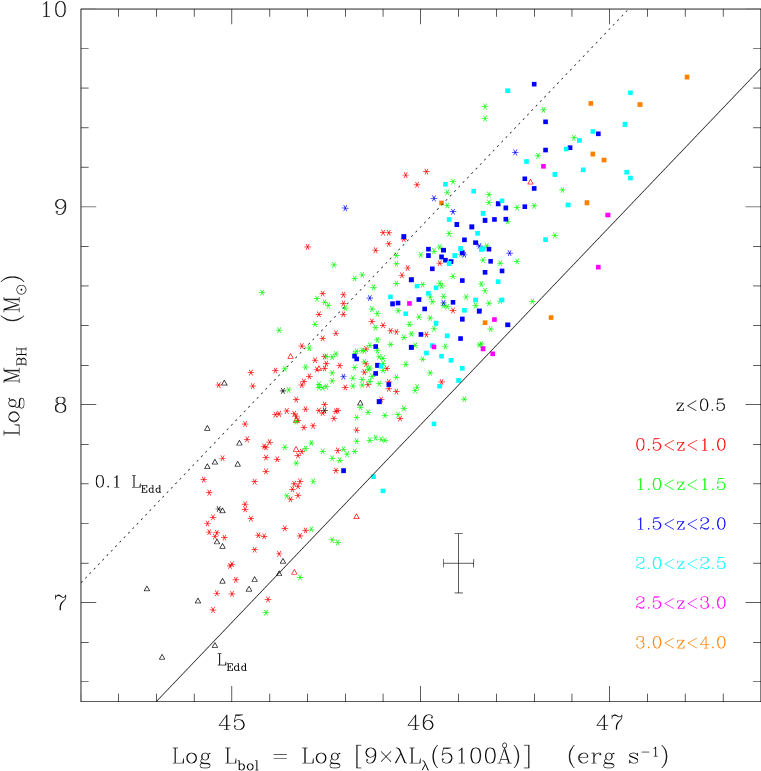
Figure 6: Estimated BH masses as a function of AGN bolometric luminosity. Objects are color-coded by redshift range as indicated in the legend. The solid line denotes the Eddington limit, $L_{\rm Edd}$; objects to the right of the line are radiating above Eddington for the measured mass. The dotted line denotes one-tenth of the Eddington limit. Point types denote the emission line used for the mass measurement, with open triangles, asterisks, and filled squares corresponding to H$\beta$, Mg II, and C IV, respectively.

Figure 6 shows the distribution of AGNs in inferred BH mass, $M_{\rm BH}$, and bolometric luminosity, $L_{\rm bol}$. The points are color-coded by redshift, and we show only a typical error bar to avoid clutter. These uncertainties reflect only the statistical errors in the line width and luminosity estimates, and we will discuss the possible consequences of systematic errors in § 5. Figure 6 has several striking features. First, it is characterized by a fairly narrow ridge that extends diagonally, with unit slope, across the entire diagram. Second, this ridge is separated from the solid line representing the Eddington limit by approximately 0.6 dex. Third, at a given luminosity, the density of points falls rapidly toward higher $M_{\rm BH}$, i.e., at small Eddington ratio. Most of the conclusions of this paper are derived by quantifying these features. At fixed $L_{\rm bol}$, the ridge is broader than the statistical uncertainties, indicating that it is dominated either by intrinsic scatter in the underlying distribution or by scatter between the inferred values of $M_{\rm BH}$ and $L_{\rm bol}$ and their true values. While the systematic errors in $L_{\rm bol}$ should be modest, determining the systematic errors in $M_{\rm BH}$ is a notoriously difficult problem to which we will return in § 5. However, from the ridge’s relatively narrow width it is already clear that this scatter cannot be too large. The fact that the ridge is displaced from the Eddington limit shows that the great majority of observed AGNs radiate at modestly sub-Eddington rates, assuming that our $M_{\rm BH}$ calibration is correct in the mean. The fact that there are few AGNs above the ridge implies that the observed (in practice, luminosity-limited) AGNs are dominated by BHs radiating close to Eddington rather than more massive BHs radiating well below Eddington. The data presented in Figure 6 also permit one to pose an orthogonal question: what is the distribution of AGN luminosities at fixed $M_{\rm BH}$? However, this question cannot be addressed by mere inspection of this figure and will require additional analysis.

AGNs rejected from the final sample due to low S/N could induce the illusion of a narrow ridge if these lay preferentially near the selection boundary. Figure 7 shows the $\log L_{{\rm bol}}$ vs. $\log M_{{\rm BH}}$ positions of the AGNs eliminated due to low S/N spectra and can be compared to Figure 6. We have not included in Figure 7 objects rejected due to absorption, Fe II emission, or other anomalous features. These objects (for which we show the $L_{{\rm bol}}$ distribution in the inset of Fig. 7) have unmeasurable FWHMs, and it therefore is not sensible to assign any mass value, in contrast to AGNs for which we simply have low confidence in the measured value. Objects were rejected without reference to their position in Figure 7, and there is no strong clustering of their position in this diagram. The simplest interpretation of this broad, flat distribution is that the FWHM measurements are simply bad, and that the calculated $M_{{\rm BH}}$ values bear only a casual relation to the true values. While the inclusion of these uniformly distributed bad measurements would slightly increase the dispersion of our measurements, we believe that their rejection is justified. In any case, including them does not qualitatively alter our results, as we show in § 4.2. Hence, we adopt the conclusions based on their exclusion.

In the next two subsections we examine the distributions of Eddington ratios at fixed $L_{\rm bol}$ (§ 4.1) and fixed $M_{\rm BH}$ (§ 4.2) as functions of redshift.

4.1 Luminosity-Redshift Bins

In order to characterize the true distributions of masses and luminosities for the BHs in our sample, we perform a very simple maximum likelihood analysis, fitting the data assuming a model in which the true distribution of $\log(L_{{\rm bol}}/L_{{\rm Edd}})$ is Gaussian (i.e., $L_{\rm bol}/L_{\rm Edd}$ is log-normal). We divide the sample into 2 bins in redshift and 3 bins in luminosity. The redshift division is at $z=1.2$, and the luminosity cuts are at $10^{45.5}~{}{\rm erg\;s^{-1}}$ and $10^{46.0}~{}{\rm erg\;s^{-1}}$ in both redshift bins. Due to the different redshift distributions of sources at high and low luminosity, it is impossible to make cuts that yield similar numbers of objects in each bin. We therefore choose cuts such that we have at least $\sim$10 objects in each bin. In each $(L_{\rm bol},z)$ bin we estimate the mean and dispersion of $\log(L_{{\rm bol}}/L_{{\rm Edd}})$, corrected for the statistical uncertainties.

The histograms in Figure 8 show the distributions of estimated $\log(L_{\rm bol}/L_{\rm Edd})$ in each $(L_{\rm bol},z)$ bin. For each panel, we calculate the unweighted mean and standard deviation of the data points, and we plot a Gaussian with those parameters as a dashed curve in the panel. Solid curves show the Gaussians with our maximum likelihood fit parameters, which account for the statistical errors in the linewidth and luminosity of each data point. Overall, these statistical errors are small compared to the widths of the histograms, so there is little difference between the dashed and solid curves. Table 1 lists the measured mean, dispersion, skewness, and kurtosis of the distributions in each $(L_{\rm bol},z)$ bin, and the mean and dispersion of the maximum likelihood Gaussian fits.

The first point to note from Figure 8 is that the distribution of $\log(L_{\rm bol}/L_{\rm Edd})$ measurements in each bin is nearly Gaussian, with a center and width that is approximately independent of redshift and luminosity. This result quantifies the impression from Figure 6 that the observed AGNs in our sample are predominantly BHs radiating fairly near Eddington ($L_{\rm bol}/L_{\rm Edd}\sim 1/4$), rather than more massive BHs at $L_{\rm bol}/L_{\rm Edd}\ll 1$. The skewness and kurtosis of the distributions are in good agreement with the values $S_{k}=0$ and $A_{k}=3$ expected for a Gaussian distribution.

The second point to note is that these Gaussians are rather narrow: $\sigma\approx 0.3$ dex after accounting for the statistical errors in our linewidth and luminosity measurements. These widths reflect the width of the intrinsic distribution of Eddington ratios at fixed luminosity and the errors introduced by our use of universal values for the bolometric correction and the spectral slope. While there may be scatter around these values or around the relationships used to derive our BH masses and AGN luminosities, that scatter already appears in Figure 6. For every object in which some quantity is underestimated by the use of the mean relation, another object will have that parameter overestimated.

The only source of scatter in the estimates of $M_{\rm BH}$ that is not fully reflected in the distribution of Eddington ratios is the difference between the observed luminosity and the time-averaged continuum luminosity in the neighborhood of the broad line for a given AGN, the latter being the quantity most appropriate for the $M_{\rm BH}$ calculation. This is because both $L_{\rm bol}$ and $M_{\rm BH}$ have a luminosity dependence.

One may show that, if the rms difference between the mean $\log L$ and the one derived from the observations is $\sigma_{\log L}$, then the dispersion in mass determinations is larger than the observed dispersion in Eddington ratios, $\sigma_{\log E}$, by

$$\sigma_{\log M}^{2}=\sigma_{\log E}^{2}+(2b-1)\sigma_{\log L}^{2}$$ (2)

where $b$ is the power-law of the luminosity-dependence in equation (1). We identify three sources of $\sigma_{\log L}$: measurement error $\sigma_{\log L,{\rm meas}}\sim 0.01$ dex, scatter due to AGN variability $\sigma_{\log L,{\rm var}}\sim 0.11$ dex, and extrapolation of the line continuum from the $R$-band measurement $\sigma_{\log L,{\rm slope}}\sim 0.04$ dex. Combining these in quadrature, and using $\sigma_{\log E}=0.30$ dex, we find $\sigma_{\log M}=0.32$ dex, which differs negligibly from $\sigma_{\log E}$. We note that this estimate of $\sigma_{\log M}$ represents the maximum possible error on $M_{\rm BH}$ and assumes that the intrinsic Eddington ratio distribution has no width of its own.

The conclusion that the quadrature sum of measurement errors in $M_{\rm BH}$, scatter in bolometric corrections, scatter in spectral slopes, and variations in $L_{\rm bol}/L_{\rm Edd}$ is only $\sim$0.3 dex rms is rather remarkable. The data give no clear indication of how to partition the scatter between these contributions. The rms scatter of 0.3 dex in inferred $M_{\rm BH}$ seems plausible on geometrical grounds, since the relation between observed linewidth and BH mass may depend on viewing angle (Krolik 2001; Collin et al. 2006; C. Kuehn & B. Peterson, in preparation). If the observational errors or the distribution of viewing angles do dominate the width of the histograms, then the intrinsic distribution of $L_{\rm bol}/L_{\rm Edd}$ is very narrow indeed.

Figure 9 compares the observed distribution in the $\log L_{\rm bol}-\log M_{\rm BH}$ plane (shown earlier in Fig. 6) to three Monte Carlo realizations in which we draw an estimated BH mass for each observed AGN from a Gaussian in $\log(L_{\rm bol}/L_{\rm Edd})$ with mean of $-0.6$ dex and dispersion of 0.3 dex. It is clear by visual inspection that this simple model describes the observed distribution of points remarkably well. While one may be tempted to see outliers or gaps in Figure 6, these features commonly appear in Monte Carlo realizations of the sample made assuming the log-normal model.

We stress that from an observational standpoint, the procedure followed in this section is extremely clean. Since the sample completeness is well-characterized at fixed optical luminosity and is independent of Eddington ratio, there are almost no selection effects coming into play in any of the luminosity bins. Application of our completeness corrections have nearly zero effect on these histograms. On the other hand, within each luminosity bin there is a contribution to the dispersion in the histogram from uncertainties in estimating $M_{\rm BH}$. The robust nature of binning by luminosity also applies to AGN surveys with other flux limits. For example, in Figure 3 of McLure & Dunlop (2004), who analyzed more than 12,000 AGNs from SDSS, one can make similar cuts at constant $\dot{M}_{\rm BH}$ ($\propto L_{\rm bol}$). McLure & Dunlop (2004) calculated the mean Eddington ratio as a function of redshift, finding the mean to increase slightly with $z$ (from 0.15 at $z\simeq 0.2$ to 0.5 at $z\simeq 2.0$), but they do not address the shape of the distribution at fixed luminosity, nor, for the redshifts that they can probe, the distribution at fixed mass. Woo & Urry (2002) find a much broader distribution of Eddington ratios in their sample of 234 AGNs compiled from the literature. Because their sample consists of low redshift ($z<1$) and local ($z<0.1$) systems, and extends to bolometric luminosities as low as $10^{43}$ erg s^-1, the difference from our results could plausibly be explained by the very different properties of the samples. The Warner et al. (2004) and Vestergaard (2004) studies of heterogeneous samples of AGNs are most akin to what we have presented here. In both works, Eddington ratios are presented over a wide range of redshifts and luminosities. However, because both studies relied on diverse mixtures of samples, the selection effects are not easily understood, and therefore, the underlying distribution of Eddington ratios cannot be determined. For example, the Warner et al. (2004) luminosity distribution is heavily weighted towards high luminosity objects. Two of the main advantages of the AGES-I survey are the homogeneity of the sample and the relatively straightforward completeness corrections (see § 2.1), which allow us to address the underlying distribution of Eddington ratios.

4.2 Mass-Redshift Bins

The distribution of Eddington ratios at fixed luminosity is a convolution of the luminosity distribution at fixed BH mass with the underlying BH mass function (see Steed & Weinberg 2003). Thus, the fall-off at low Eddington ratios in Figure 8 could, in principle, be attributed primarily to a rapid fall-off in the $M_{\rm BH}$ distribution toward higher masses. Since we know from our previous discussion that the errors in BH mass assignments must be fairly small (0.3 dex rms at most), we can bin the sample by estimated BH mass and look directly at the distribution of Eddington ratios at fixed $M_{\rm BH}$. Figure 10 shows these distributions for mass bins $\log(M_{\rm BH}/M_{\odot})=7-8$, $8-9$, and $9-10$, and redshift bins $z=1-2$, $2-3$, and $3-4$.

In contrast to Figure 8, the distribution of Eddington ratios at fixed mass is affected by the magnitude limit of the survey. We also must include the effects of incompleteness at the faint end. We use the completeness function of Figure 1 and the $R$-band magnitude of each of our 407 AGNs to calculate the number of objects at each observed combination of $L_{{\rm bol}}$ and $z$ that are “missing”. The missing objects are then distributed in mass at the ($L_{{\rm bol}}$,$z$) of the real AGN via the Eddington ratio distribution we found in § 4.1. For all objects, we take the distribution as log-normal in $L_{\rm bol}/L_{\rm Edd}$, with a mean of 1/4 and with $\sigma$=0.30 dex. The contribution of these missing objects to each bin of Eddington ratio is then summed within the mass and redshift ranges chosen for each panel. The solid histograms in each panel are completeness-corrected. This alters the histograms, but does not substantially alter our conclusions. The vertical arrow in each panel of Figure 10 indicates the point in that mass-redshift bin at which AGNs are first lost to optical selection effects (which begin at the low-$M_{\rm BH}$, high-$z$ corner of the bin), and the shaded region indicates the point at which all AGNs (extending to the highest $M_{\rm BH}$ and lowest $z$ corner of the bin) are lost. For the lower-mass bins (particularly at high redshift), the optical magnitude limit truncates the distributions, and we cannot determine whether there is a true cutoff at low $L_{\rm bol}/L_{\rm Edd}$. However, in some bins, the optical magnitude limit only affects the regime $L_{\rm bol}/L_{\rm Edd}\lesssim 0.1$, and it is possible to test for a real cutoff. In the highest-mass highest-redshift bin of Figure 10, there are too few objects to make a robust determination. However, Figure 11 shows four bins — $\log(M_{\rm BH}/M_{\odot})=8.5-10$ at $z=0.75-1$ and $1.5-2$, $\log(M_{\rm BH}/M_{\odot})=8.75-10$ at $z=1-1.5$, and $\log(M_{\rm BH}/M_{\odot})=9-10$ at $z=2-3$ — in which the statistics are relatively good and the fall-off appears to be real. The Poisson probabilities that the peak in each case is a statistical fluctuation are found to be low, as shown in each panel in Figure 11. The peak is therefore robust and not merely a product of counting statistics.

Finally, Figure 12 shows the effect of including the low S/N measurements from Figure 7 on our Eddington ratio distributions at fixed mass. The low S/N spectra do not affect any of our conclusions above.

We note that the scatter in inferred $M_{\rm BH}$ might move AGNs from one mass bin to another, which could potentially enhance the appearance of a peak either on the rising or the falling sides. Recall from § 4.1 and Table 1 that the rms scatter in the inferred $M_{\rm BH}$ must be less than $\sim$0.3 dex. Because the mass bins in Figure 11 have widths of at least 1 dex, scatter between mass bins must be a small effect. The smooth distribution of Eddington ratios seen in Figure 6 implies that it would be difficult to import structure into or out of a particular mass bin without having significant structure in another part of the distribution from which objects can scatter. No such structure is seen in our data. In fact, if we bin the Monte Carlo realizations of Figure 9, which have a $\sigma=0.3$ dex Gaussian distribution of estimated $\log(L_{{\rm bol}}/L_{{\rm Edd}})$ and which match the sample’s observed luminosity distribution by construction, then we get histograms that qualitatively resemble those in the four mass-redshift bins of Figure 11. This simple model therefore appears consistent with our data, although this experiment on its own does not tell us whether the observed distributions are shaped primarily by intrinsic scatter in $L_{\rm bol}/L_{\rm Edd}$ or by errors in $M_{\rm BH}$ estimation.

The filled circles at the bottom of each panel in Figures 10 and 11 show the relevant spectroscopic limit of the SDSS for each redshift bin. The SDSS data are not deep enough to probe the cutoff in any of these bins, i.e., the SDSS cannot provide an unbiased study of the Eddington ratio distribution below 0.1 for BHs with $M_{\rm BH}<10^{9}M_{\odot}$ above $z\sim 1$, or $M_{\rm BH}<10^{9.6}M_{\odot}$ above $z\sim 2$. Because of its large area, the SDSS can obtain better statistics for high mass BHs at low redshift, or for very massive BHs at higher redshift, and it will be interesting to see whether these have a peaked Eddington ratio distribution similar to that found here.

4.3 Mg II Scaling

The calibration of Mg II presents a potential problem for the conclusions drawn from the AGES-I data that make use of this line. Our empirical calibration leads to a steeper dependence of $M_{{\rm BH}}$ on luminosity for the Mg II relationship (§ 3.3) than for C IV or H$\beta$. As pointed out by Woo & Urry (2002), if the dependence of black hole mass on luminosity is nearly linear and there is a simple relationship between the continuum and bolometric luminosities, then a strong correlation of increasing $M_{\rm BH}$ with increasing $L_{\rm bol}$ will be automatically introduced. With such a scaling relation, it would be possible for a small, but random distribution of Mg II FWHMs to reproduce a tight Eddington ratio distribution without actually being related to the BH mass. However, the clear trend in Figure 4 and the fact that the Mg II relation scales as $V^{2}$, even when the velocity dependence is allowed to vary, indicates that the relationship among the 3000 Å continuum luminosity, the Mg II line width, and the black hole mass is not random.

Our empirical calibration for Mg II depends directly on what we use for the H$\beta$ and C IV relations. A new calibration of those two emission lines has recently been published (Vestergaard & Peterson, 2006), which has derived shallower slopes for both the H$\beta$ and C IV luminosity scalings, with ($a,b$) values of (0.91, 0.50) and (0.66, 0.53), respectively. The effect of adopting those relations is to shift the H$\beta$ points up $\sim$0.2 dex in mass (as they have typical luminosities near 10⁴⁵ erg s^-1), and to shift the C IV points up by $\sim$0.28 dex at the low luminosity end ($\sim 10^{46}$ erg s^-1), and to leave them nearly unchanged at the high luminosity end. Using these relations then sets the parameters of our empirically calibrated Mg II mass relation to (0.55, 0.82). This shift produces roughly coherent movement across the $M_{{\rm BH}}-L_{{\rm bol}}$ plane, so the shapes of our histograms at fixed mass are basically unaffected—although our highlighted bins in Figure 11 must be shifted upwards by $0.25-0.5$ dex in mass.

5 Discussion

Our survey of $R\leq 21.5$ mag, X-ray- and 24$\micron$-selected AGNs in the Boötes NDWFS field yields four basic results. First, the rms scatter in BH masses inferred from linewidth-luminosity scaling relations is less than 0.3 dex, at least for $M_{\rm BH}>10^{8}M_{\odot}$ and the luminosity range $L_{\rm bol}\sim 10^{45}-10^{47}$ erg s^-1. Second, luminous AGNs at $z>0.5$ are powered by BHs radiating at roughly $1/4$ of the Eddington rate: there are few cases of higher mass BHs radiating well below Eddington or of lower mass BHs radiating well above Eddington. Third, at fixed mass above $10^{8.5}~{}M_{\odot}$ (where selection effects are inconsequential), the distribution of Eddington ratios at $z>0.75$ is strongly peaked. Fourth, the distribution around this peak is confined to within $\sim 1$ dex in $L_{{\rm bol}}/L_{{\rm Edd}}$, with many fewer broad-lined AGNs on either side.

Our analysis does not test the zero-point or luminosity scaling of the $M_{\rm BH}$ relations. To aid comparisons with previous work, we have used the scaling relations of McLure & Jarvis (2002) for H$\beta$ and Vestergaard (2004) for C IV. The results of Onken et al. (2004), in which reverberation-based BH masses were calibrated by assuming that AGNs follow the same correlation between BH mass and stellar velocity dispersion as quiescent galaxies, suggest that the zero points of these relations should be adjusted upward by factors of 1.4 and 1.8, respectively. We did adjust the McLure & Jarvis (2002) Mg II relation based on the empirical evidence for a different luminosity scaling, as shown in Figure 4. Altering the zero-points of the $M_{\rm BH}$ relations or the mean bolometric correction would change our conclusions about the location of peaks in the $L_{\rm bol}/L_{\rm Edd}$ distributions, but they would not change our conclusions about the existence of these peaks. For example, the Onken et al. (2004) revision would shift the means of our $L_{\rm bol}/L_{\rm Edd}$ distributions downward by $\sim 0.2$ dex, but would not broaden the distributions (this shift has been incorporated into the analysis of Vestergaard & Peterson 2006.) With an identical shift to the mass ranges in Figure 11, the relative positions of the histograms and the arrows in each panel would remain the same, but everything would be at a slightly lower Eddington ratio. Given the numerous complexities of BH mass estimates from emission line widths, our empirical evidence that these estimates have less than 0.3 dex rms scatter is remarkable. One might expect scatter nearly this large from geometrical effects alone, since the relation between observed linewidth and the BH mass may depend on viewing angle.

The dominance of the $z>0.5$ AGN population by near-Eddington accretors is very different from the local-universe sample of AGNs, for which the distribution of inferred Eddington ratios is broader (e.g.,Woo & Urry 2002; Ho 2004; Heckman et al. 2004). The luminosities of these local AGNs are typically much lower than those in our sample, so it is unclear whether luminosity or redshift dependence is responsible for most of the difference. The AGES-I sample does not probe down to Seyfert luminosities (below $\sim 10^{44}\;{\rm erg}\;{\rm s}^{-1}$), and we therefore cannot comment on the contribution of broad-lined Seyfert galaxies to the overall black hole growth. In addition, while narrow-line objects cannot be analyzed using the methods employed here, they are a very small fraction of the overall AGES-I AGN sample, with only 29 objects in the range $0.5\leq z\leq 1$ matching a narrow-line template and no such objects above $z=1$. High Eddington ratios for the most luminous quasars at high redshift are not surprising, since the steep high-mass fall-off of the BH mass function (see, e.g., Aller & Richstone 2002) means that the BHs required to power them at sub-Eddington luminosities would be very rare. However, the dominance of near-Eddington accretors at the knee of the luminosity function and at redshifts at which the quasar luminosity function is declining in amplitude imposes strong constraints on the distribution of BH fueling rates (Steed & Weinberg, 2003). Of course, there must also be many BHs with much lower $L_{\rm bol}/L_{\rm Edd}$ (perhaps approaching zero), otherwise it would be hard to reconcile the local BH mass function with the observed number of AGNs. However, these low Eddington-ratio objects do not contribute significantly to the observed AGN population in the luminosity and redshift range probed by AGES-I.

For high mass BHs at $z>1$, we can make these constraints more direct by computing the $L_{\rm bol}/L_{\rm Edd}$ distributions at fixed BH mass. The depth of the AGES-I survey is crucial in allowing us to compute histograms for $L_{\rm bol}/L_{\rm Edd}>0.1$ that are unaffected by the survey magnitude limit (see Fig. 11). Accounting for completeness corrections, these histograms clearly decline toward both high and low $L_{\rm bol}/L_{\rm Edd}$ from the peak. This peak could be further studied by the expansion of the AGES survey presently underway (AGES-II) and the 2SLAQ survey, which probes to approximately the same depth as AGES-I over a much wider area (Richards et al., 2005). However, because 2SLAQ AGNs are selected by optical colors, the effects of dust extinction may be more severe for this survey than for AGES.

Our results strongly suggest that BHs gain most of their mass while accreting at near-Eddington rates. Since the height of the Eddington ratio distribution falls as $L_{\rm bol}/L_{\rm Edd}$ drops from 0.3 to 0.1, any rise at lower values would have to be extremely steep to contribute more mass growth than the observed peak. The main loopholes are the possibilities that much of the growth occurs in objects that are obscured at optical wavelengths or are accreting with very low efficiency. Such objects could plausibly have a different $L_{\rm bol}/L_{\rm Edd}$ distribution. However, the reasonable agreement between the integrated emissivity of the optical quasar population and the local BH mass density (Soltan 1982; see Shankar et al. 2004 for a recent analysis) suggests that any such population cannot dominate by a large fraction. In fact, the Shankar et al. (2004) analysis concluded that Eddington ratios of $\sim 1/3$ at $z=3$ were required in order to obtain a good match between the emissivity from optical quasars and the local BH mass density. We also note that our AGN sample is not as adversely affected by obscuration effects as most existing surveys. While the X-ray-selected AGNs are affected by soft X-ray absorption, the 24$\micron$-selected AGNs are not. Furthermore, the bluest optical band used for target selection in this survey is the $R$-band instead of the more commonly used optical $B$-band. This relative immunity to obscuration will be enhanced further in the AGES-II AGN sample, which will have an optical flux limit ($I=21.5$ mag) that is both at a longer wavelength and deeper.

For a BH to become active, some event (merger, tidal interaction, dynamical instability, etc.) must drive material into the central few parsecs of its host galaxy, and this inner material must then form an accretion flow onto the BH itself, on the much smaller scale of hundreds to thousands of AU. The galactic-scale fueling events are likely to have a broad mass distribution, and there is no reason for them to know about the precise mass of the central BH. The sharp peak of the observed $L_{\rm bol}/L_{\rm Edd}$ distribution suggests that these events are often sufficient to provide super-Eddington fuel supplies and that the actual BH accretion rates are determined by the BH’s self-regulation of the inner accretion flow. The narrow width ($\leq 0.3$ dex) and central value ($L_{\rm bol}/L_{\rm Edd}\sim 1/4$) are important targets for theoretical models of accretion flows, though further investigation of the zero-point calibration of $M_{\rm BH}$ indicators is desirable to firm up the latter constraint. Overall, the population of active BHs in the AGES-I survey is simpler than one might have imagined beforehand, and explaining this simplicity is a new challenge for theories of AGN evolution.

Figure 1: Completeness correction as a function of $R$-band magnitude. The solid line shows our overall completeness correction. The dashed line shows the AGES-I completeness relative to AGES-II. The departure between the two lines shows where we make an additional correction for loss of blue objects due to the AGES-II 3.6$\micron$ flux limit.

Figure 2: Illustration of the method for measuring the FWHMs. Blue1 and Red1 indicate the wavelengths of the first crossing of the half-max point descending from the line peak, and Blue2 and Red2 show the first half-max crossing ascending from the line limits. Red1 and Red2 are averaged to produce the wavelength Red. In this cartoon, Blue1 and Blue2 are identical and so are equal to Blue. The FWHM is determined by the difference between Red and Blue.

Figure 3: Examples of typical smoothed spectra. Panels from top to bottom show examples of an acceptable spectrum, a spectrum rejected for low S/N, a spectrum with strong Fe II emission, and a spectrum with strong absorption.

Figure 4: Comparison of BH masses derived from the McLure & Jarvis (2002) Mg II scaling relation and our adopted H$\beta$ (open triangles) or C IV (filled squares) scaling relations in redshift regimes of overlap, as a function of bolometric luminosity, $L_{\rm bol}$. The line shows the best fit to the combined dataset and forms the basis for our modified calibration of the Mg II relation.

Figure 5: AGN luminosity as a function of redshift. Points are coded according to the emission line used for the mass measurement, with open triangles, asterisks, and filled squares corresponding to H$\beta$, Mg II, and C IV, respectively. Also shown are solid curves at $R$ = (17, 19, 21) mag, the SDSS spectroscopic flux limit as a function of redshift (dashed line; $z<3$: $R\approx 18.9~{}{\rm mag}$, $z>3$: $R\approx 20.0~{}{\rm mag}$), and the AGES-I spectroscopic limit (dotted line; $R$=21.5 mag). The dot-dashed line shows the evolution of the knee in the luminosity function with redshift, as determined by the 2SLAQ survey (Richards et al., 2005).

Figure 7: Estimated BH masses as a function of AGN bolometric luminosity. Points show objects eliminated from our final sample in cases for which the S/N of our data was insufficient to make a reliable FWHM measurement. Point types are as in Figure 6. The histogram below shows the luminosity distribution of objects for which no sensible FWHM determination could be made (independent of the quality of the spectrum).

Figure 8: Distributions of Eddington ratios in bins of luminosity and redshift. The panels are divided between $z<1.2$ (left) and $z>1.2$ (right) and in increasing luminosity from bottom to top. The histograms show the fraction of data points at each value of $L_{bol}/L_{\rm Edd}$. Dashed curves are Gaussians with the same mean and dispersion as the data. Solid curves are the best-fit Gaussians, accounting for measurement uncertainties in luminosity and linewidth. These curves are similar because the measurement errors are small compared to the distribution widths. At all redshifts and luminosities, we find that most AGNs are radiating close to Eddington, with a dispersion of only $\sim 0.3$ dex.

Figure 9: Monte Carlo realizations of BH mass vs. bolometric luminosity. The upper left panel shows the actual data, repeated from Fig. 6. The remaining panels are 3 different Monte Carlo realizations of our data in which we retain our observed luminosities and draw the $\log(L_{\rm bol}/L_{\rm Edd})$ (and hence $M_{{\rm BH}}$) value for each AGN from a single Gaussian distribution with mean $\mu=-0.6$ and dispersion $\sigma=0.3$. The distribution of points in the simulated datasets supports our inference from Fig. 8, that a single, narrow Gaussian is an adequate description of the data.

Figure 10: Distribution of Eddington ratios in bins of fixed BH mass and redshift. Panels from left to right show 3 bins in mass, each 1 decade wide, ranging over $M_{\rm BH}=10^{7-10}M_{\odot}$. Panels from top to bottom show the redshift ranges $3<z<4$, $2<z<3$, and $1<z<2$. The solid histograms in each panel show the distributions for the “clean” dataset of 407 objects corrected for completeness. The dotted histograms show our data prior to the completeness-correction. The arrows show where AGNs within the bin are first hitting the optical flux limit. The shaded regions mark where AGNs are completely lost to optical selection. The position of the solid dots along the bottom of each panel show the equivalent of the arrows for the SDSS spectroscopic flux limit for that bin (in the lowest mass bins, these lie to the right of the plotted $x$-axis range).

Figure 11: Eddington ratio distribution at fixed mass in bins for which distribution shape is not determined by optical selection. The mass and redshift range for the bin is designated within each panel. Solid histograms show our completeness-corrected values and dotted lines correspond to our raw measurements. The arrows show where AGNs within the bin are first hitting the optical flux limit. The solid dots along the bottom of each panel show the equivalent of the arrows for the SDSS spectroscopic limit for that bin. The Poisson probabilities listed in each panel reflects the chance that the peak height of the solid histograms is produced by small number statistics alone.

Figure 12: Effect of object removal on the peak in Eddington ratio distribution at fixed mass in bins for which distribution shape is not determined by optical selection. The mass and redshift range for each bin is designated within each panel. Solid lines show our completeness-corrected measurement as in Fig. 11 and dashed histograms include objects removed for low S/N (also corrected for completeness). The arrows show where AGNs within the bin are first hitting the survey optical flux limit. The solid dots along the bottom of each panel shows the equivalent of the arrows for the SDSS spectroscopic flux limit for that bin. The Poisson probabilities listed in each panel reflects the chance that the peak height of the dashed histograms is produced by small number statistics alone.

Table 1: Gaussian Parameters of Data and Fits to Data

$z_{\rm bin}$	$L_{\rm bin}$	$N$	$\mu_{\rm data}$	$\sigma_{\rm data}$	$S_{k}$	$A_{k}$	$\mu_{\rm model}$	$\sigma_{\rm model}$
Low	Low	115	$-$0.61	0.35	0.01	2.69	$-$0.62	0.32
High	Low	9	$-$0.66	0.38	0.08	1.78	$-$0.70	0.32
Low	Med	65	$-$0.62	0.33	$-$0.07	2.49	$-$0.63	0.30
High	Med	65	$-$0.56	0.29	$-$0.17	3.77	$-$0.57	0.27
Low	High	22	$-$0.55	0.34	$-$0.27	2.55	$-$0.54	0.33
High	High	131	$-$0.52	0.28	$-$0.02	2.87	$-$0.52	0.24

Note. — For each bin in redshift, $z_{\rm bin}$, and luminosity, $L_{\rm bin}$, the table lists the number of objects, $N$, the mean Eddington ratio, $\mu_{\rm data}$, the dispersion in Eddington ratios, $\sigma_{\rm data}$, the skewness of the distribution, $S_{k}$, the kurtosis of the distribution, $A_{k}$, the maximum likelihood fit to the mean Eddington ratio, $\mu_{\rm model}$, and the maximum likelihood fit to the dispersion in Eddington ratios, $\sigma_{\rm model}$. In addition, we give the formulae for the errors in the mean, skew, and kurtosis.

References

- Aller & Richstone (2002) Aller, M. C., & Richstone, D. 2002, AJ, 124, 3035
- Baldwin et al. (1981) Baldwin, J. A., Phillips, M. M., & Terlevich, R. 1981, PASP, 93, 5
- Bentz et al. (2006) Bentz, M. C., Peterson, B. M., Pogge, R. W., Vestergaard, M., & Onken, C. A. 2006, ApJ, in press (astro-ph/0602412)
- Brand et al. (2006) Brand, K., et al. 2006, ApJ, 641, 140
- Collin et al. (2006) Collin, S., Kawaguchi, T., Peterson, B. M., & Vestergaard, M. 2006, A&A, in press (astro-ph/0603460)
- Corbett et al. (2003) Corbett, E. A., et al. 2003, MNRAS, 343, 705
- Clavel et al. (1991) Clavel, J., et al. 1991, ApJ, 366, 64
- de Vries et al. (2005) de Vries, W. H., Becker, R. H., White, R. L., & Loomis, C. 2005, AJ, 129, 615
- Dibai (1980) Dibai, É. A. 1980, Astron. Zh., 57, 677 (English translation: Sov. Astron., 24, 389)
- Dietrich & Kollatschny (1995) Dietrich, M., & Kollatschny, W. 1995, A&A, 303, 405
- Dietrich et al. (2002) Dietrich, M., Hamann, F., Shields, J. C., Constantin, A., Vestergaard, M., Chaffee, F., Foltz, C. B., & Junkkarinen,V. T. 2002, ApJ, 581, 912
- Dietrich & Hamann (2004) Dietrich, M., & Hamann, F. 2004, ApJ, 611, 761
- Eisenhardt et al. (2004) Eisenhardt, P. R., et al. 2004, ApJS, 154, 48
- Elvis et al. (1994) Elvis, M., et al. 1994, ApJS, 95, 1
- Fabricant et al. (1998) Fabricant, D. G., Hertz, E. N., Szentgyorgyi, A. H., Fata, R. G., Roll, J. B., & Zajac, J. M. 1998, Proc. SPIE, 3355, 285
- Fabricant et al. (2005) Fabricant, D. et al. 2005, PASP, 117, 1411
- Francis et al. (1991) Francis, P. J., Hewett, P. C., Foltz, C. B., Chaffee, F. H., Weymann, R. J., & Morris, S. L. 1991, ApJ, 373, 465
- Heckman et al. (2004) Heckman, T. M., Kauffmann, G., Brinchmann, J., Charlot, S., Tremonti, C., & White, S. D. M. 2004, ApJ, 613, 109
- Ho (2004) Ho, L. C. 2004, in Carnegie Observatories Astrophysics Series, Vol. 1: Coevolution of Black Holes and Galaxies, ed. L. C. Ho (Cambridge: Cambridge Univ. Press), 293 (astro-ph/0401527)
- Jannuzi & Dey (1999) Jannuzi, B. T. & Dey, A. 1999, in ASP Conf. Ser. 191: Photometric Redshifts and the Detection of High Redshift Galaxies, ed. R. Weymann, L. Storrie-Lombardi, M. Sawicki, & R. Brunner, 111
- Kaspi et al. (2005) Kaspi, S., Maoz, D., Netzer, H., Peterson, B. M., Vestergaard, M., & Jannuzi, B. T. 2005, ApJ, 629, 61
- Kaspi et al. (2000) Kaspi, S., Smith, P. S., Netzer, H., Maoz, D., Jannuzi, B. T., & Giveon, U. 2000, ApJ, 533, 631
- Kaspi et al. (1996) Kaspi, S., Smith, P. S., Maoz, D., Netzer,H., Jannuzi, B. T. 1996, ApJ, 471, L75
- Kenter et al. (2005) Kenter, A., et al. 2005, ApJS, 161, 9
- Kochanek et al. (2004) Kochanek, C. S., Eisenstein, D., Caldwell, N., Cool, R., Green, P., & AGES 2004, American Astronomical Society Meeting Abstracts, 205
- Koratkar & Gaskell (1991) Koratkar, A. P., & Gaskell, C. M. 1991, ApJ, 370, L61
- Krolik (2001) Krolik, J., 2001, ApJ, 551, 72
- Lynden-Bell (1969) Lynden-Bell, D., 1969, Nature 223, 690
- McLure & Dunlop (2004) McLure, R. J., & Dunlop, J. S. 2004, MNRAS, 352, 1390
- McLure & Jarvis (2002) McLure, R. J., & Jarvis, M. J. 2002, MNRAS, 337, 109
- Murray et al. (2005) Murray, S. S., et al. 2005, ApJS, 161, 1
- Onken et al. (2004) Onken, C. A., Ferrarese, L., Merritt, D., Peterson, B. M., Pogge, R. W., Vestergaard, M., & Wandel, A. 2004, ApJ, 615, 645
- Onken & Peterson (2002) Onken, C. A., & Peterson, B. M. 2002, ApJ 572, 746
- Peterson (2001) Peterson, B. M. 2001, in Advanced Lectures on the Starburst-AGN Connection, ed. I. Aretxaga, D. Kunth, & R. Mújica (Singapore: World Scientific), 3 (astro-ph/0109495)
- Peterson & Wandel (2000) Peterson, B. M., & Wandel, A. 2000, ApJ, 540, L13
- Peterson et al. (2004) Peterson, B. M., et al. 2004, ApJ, 613, 682
- Richards et al. (2005) Richards, G. T., et al. 2005, MNRAS, 360, 825
- Richards et al. (2006) Richards, G. T., et al. 2006, ApJS, submitted (astro-ph/0601558)
- Rieke et al. (2004) Rieke, G., et al., 2004, ApJS, 154, 25
- Roll et al. (1998) Roll, J. B., Fabricant, D. G., & McLeod, B. A., 1998, SPIE, 3355, 324
- Salpeter (1964) Salpeter, E., 1964, ApJ, 140, 796
- Shankar et al. (2004) Shankar, F., Salucci, P., Granato, G. L., DeZotti, G., & Danese, L. 2004, MNRAS, 354, 1020
- Soifer et al. (2004) Soifer, B. T. & Spitzer/NOAO Team 2004, American Astronomical Society Meeting Abstracts, 204
- Soltan (1982) Soltan, A. 1982, MNRAS, 200, 115
- Steed & Weinberg (2003) Steed, A., & Weinberg, D. H. 2003, ApJ, submitted, (astro-ph/0311312)
- Stern et al. (2005) Stern, D., et al. 2005, ApJ, 631, 163
- Vanden Berk et al. (2001) Vanden Berk, D., et al. 2001, AJ, 122 549
- Veilleux & Osterbrock (1987) Veilleux, S., & Osterbrock, D. E. 1987, ApJS, 63, 295
- Vestergaard (2002) Vestergaard, M. 2002, ApJ, 571, 733
- Vestergaard (2004) Vestergaard, M. 2004, ApJ, 601, 676
- Vestergaard & Peterson (2006) Vestergaard, M. and Peterson, B., 2006, ApJ, 641, 140
- Wandel, Peterson & Malkan (1999) Wandel, A., Peterson, B. M., & Malkan, M. A. 1999, ApJ, 526, 579
- Warner et al. (2004) Warner, C., Hamann, F., & Dietrich, M. 2004, ApJ, 606, 136
- Woo & Urry (2002) Woo, J., & Urry, C. M. 2002, ApJ, 579, 530
- Yu & Tremaine (2002) Yu, Q. & Tremaine, S. 2002, MNRAS, 335, 965
- Zel’dovich & Novikov (1964) Zel’dovich, Y. B., & Novikov, I. D. 1964, Dokl. Akad. Nauk SSSR, 158, 811 (English translation: 1965, Sov. Phys. Dokl., 9, 834)