Non-Gaussianity in Curvaton Models with Nearly Quadratic Potential

Abstract:

We consider curvaton models with potentials that depart slightly from the quadratic form. We show that although such a small departure does not modify significantly the Gaussian part of the curvature perturbation, it can have a pronounced effect on the level of non-Gaussianity. We find that unlike in the quadratic case, the limit of small non-Gaussianity, $|f_{NL}|\ll 1$ , is quite possible even with small curvaton energy density $r\ll 1$ . Furthermore, non-Gaussianity does not imply any strict bounds on $r$ but the bounds depend on the assumptions about the higher order terms in the curvaton potential.

1 Introduction

Possible non-Gaussian features of the Cosmic Microwave Background (CMB) temperature anisotropy can provide important constraints on models of inflation. For instance, an observation of a significant non-Gaussianity would effectively rule out single-field inflation (for a review of non-Gaussianity, see [1]). Usually in the literature the non-Gaussianities are characterized by a non-linearity parameter $f_{NL}$, which is a measure of the non-Gaussian curvature perturbation relative to the Gaussian perturbation. Present WMAP observations yield the limit [2] $-58<f_{NL}<134$ at $95\%$ confidence level. With polarization measurements, the Planck Surveyor Mission is expected to push the limit down to $|f_{NL}|\lesssim 2.9$ [3]. For the single field inflation one obtains $f_{NL}$ which is of the order of the slow-roll pararameters [4]; hence a detection of non-Gaussianity by Planck would indeed suffice to rule out single-field inflation.

For the curvaton models [5, 6, 7] it has been suggested [8] that a non-observation of non-Gaussianity would indicate that the model is ruled out, at least in the case of the quadratic potential. In curvaton models the curvature perturbation is generated after inflation by the decay of an effectively massless scalar field $\sigma$ different from the inflaton. The curvaton energy density remains subdominant until the end of inflation so that the density parameter $r\equiv 4\rho_{\sigma}/(4\rho_{r}+3\rho_{\sigma})\ll 1$, where $\rho_{r}$ is the energy density of radiation after inflation. Thereafter the curvaton field begins to oscillate and behaves effectively like matter. Its relative energy density grows during oscillations and when it eventually decays, the perturbation it has received during inflation will be imprinted on the decay products, the light degrees of freedom. Because the curvaton is massless, the perturbation is predominantly Gaussian. However, there will also be a non-Gaussian contribution that arises because of the curvaton dynamics after inflation. By now a well-known result is that in curvaton models with quadratic potential the non-linearity parameter can be written as [8, 11]

$$f_{NL}=\frac{5}{3}+\frac{5}{8}r-\frac{5}{3r}~{}.$$ (1)

Thus, for low $r$ as required for the subdominance of the curvaton during inflation, $|f_{NL}|$ is typically much bigger than 1. However, we wish to point out that this result is considerably modified for non-quadratic potentials. Although the curvaton must be weakly self-interacting, it is highly likely that there is some departure from the quadratic potential. As we will discuss in this paper, while leaving the Gaussian perturbation essentially unchanged, a small correction to the quadratic potential can have an important effect on the non-Gaussianity parameter. Indeed, we show that if one does not insist on a strictly quadratic potential, it is quite possible to have $|f_{NL}|$ much less than 1 also in the curvaton scenario.

2 The curvature perturbation generated in the curvaton model

We adopt here the non-linear, the so-called separate universe approach presented in [10, 12, 13, 14], which is valid on large scales. There one considers perturbations around the homogeneous and isotropic flat FRW-universe assuming that their spatial variation outside horizon is smooth. The evolution of large scales is approximated by replacing each quantity by its spatial average inside some smoothing scale $k^{-1}_{\rm smooth}$ and considering these smoothed, locally homogeneous and isotropic regions to evolve like separate FRW-universes [10, 13, 14]. The spatial variation of perturbations outside the smoothing scale is taken into account by doing first order gradient expansion leading to different expansion rates in different smoothed regions. Here we briefly recapitulate the main features [10, 14] of this approach relating to non-Gaussianity in curvaton models.

In the first order in gradient expansion, the spatial part of the metric can be written as [14]

$$g_{ij}=a^{2}(t)e^{-2\psi(t,{\bf x})}\gamma_{ij}$$ (2)

where $\gamma_{ij}$ is constant, assuming the amplitude of the gravitational waves to be small. The curvature perturbation $\psi(t,{\bf x})$ thus defined can be interpreted as a perturbation in the scale factor, $\tilde{a}(t,{\bf x})\equiv a(t)e^{-\psi(t,{\bf x})}$. As it has been shown in [10, 14], the curvature perturbation on uniform energy density hypersurfaces stays constant outside the horizon in the absence of non-adiabatic pressure perturbation; just like its counterpart in the usual first [15] and second order perturbation theories [16].

The amount of expansion along the worldline of a comoving observer from a spatially flat $\psi=0$ slice at time $t_{1}$ to a generic slice at time $t$ is given by $N(t,{\bf x})={\rm ln}\frac{\tilde{a}(t,{\bf x})}{a(t_{1})}$ since the expansion in a spatially flat gauge corresponds to that of the unperturbed universe. By choosing the slice at time $t$ to have uniform energy density, the curvature perturbation on that slice can be written as [10, 14]

$$\zeta(t,{\bf x})\equiv-\psi(t,{\bf x})={\rm ln}\frac{\tilde{a}(t,{\bf x})}{{a}(t)}=N(t,{\bf x})-N(t)$$ (3)

where $N(t)$ is the amount of expansion in the background universe.

Following [10] we expand the curvature perturbation (3) up to second order in the Gaussian curvaton perturbations in order to take into account the non-Gaussian effects:

$$\zeta(t,{\bf x})=\partial_{\sigma}N(t)\delta\sigma(t,{\bf x})+\frac{1}{2}\partial^{2}_{\sigma}N(t)\delta\sigma(t,{\bf x})^{2}.$$ (4)

In the limit $r\ll 1$ the curvature perturbation is almost completely generated during oscillations of the curvaton field. Assuming sudden decay at $t=t_{\rm dec}$ the amount of expansion in the background universe during oscillations is given by [10]

$$N(\sigma_{\rm dec},\sigma_{\rm osc})=\frac{1}{3}{\rm ln}\frac{\frac{1}{2}m_{\sigma}\sigma^{2}_{\rm osc}}{\frac{1}{2}m_{\sigma}\sigma^{2}_{\rm dec}}=\frac{1}{4}{\rm ln}\frac{(\rho_{r})_{\rm osc}}{\rho_{\rm dec}-(\rho_{\sigma})_{\rm dec}}$$ (5)

where $\sigma_{\rm osc}$ is the value of the curvaton at the onset of oscillations. The total curvature perturbation is obtained by substituting Eq. (5) into Eq. (4)

$$\zeta(t,{\bf x}) = \frac{r\sigma^{\prime}_{\rm osc}}{2\sigma_{\rm osc}}\delta\sigma_{*}+\frac{1}{4}\Big{(}\Big{(}-\frac{3}{8}r^{3}-r^{2}+r\Big{)}\Big{(}\frac{\sigma^{\prime}_{\rm osc}}{\sigma_{\rm osc}}\Big{)}^{2}+r\frac{\sigma^{\prime\prime}_{\rm osc}}{\sigma_{\rm osc}}\Big{)}\delta\sigma^{2}_{*}$$ (6)

where we have denoted $\partial_{\sigma_{*}}\equiv^{\prime}$ . The initial values for the curvaton field $\delta\sigma_{*}(t,{\bf x})$ in each smoothed region are set by inflation and the derivatives in Eq. (4) are thus taken w.r.t the field value during inflation $\sigma_{*}$.

We point out that the nonlinear part in the curvature perturbation, Eq. (6), consists of a square of the linear part $(\frac{\sigma^{\prime}_{\rm osc}}{\sigma_{\rm osc}}\delta\sigma_{*})^{2}$ and of an additional dynamical term. One could thus expect that the non-Gaussian effects would be more dependent on the dynamics than the Gaussian part which is indeed quite reasonable since, loosely speaking, the Gaussian part depends on the size of the perturbations while the non-Gaussian part depends on the relative size of the perturbations compared to the background field.

From Eq. (6) the curvature perturbation can be written in the form [17] $\zeta=\zeta_{g}-\frac{3}{5}f_{NL}(\zeta_{g}^{2}-\langle\zeta_{g}^{2}\rangle)$ where $\zeta_{g}$ is Gaussian and the non-linearity parameter $f_{NL}$ is independent of position. The non-linearity parameter can now be directly read off from Eq. (6):

$$f_{NL}=\frac{5}{3}+\frac{5}{8}r-\frac{5}{3r}\Big{(}1+\frac{\sigma^{\prime\prime}_{\rm osc}\sigma_{\rm osc}}{\sigma^{\prime 2}_{\rm osc}}\Big{)}.$$ (7)

Although this result was obtained in [10, 18], the dependence of the last term ${\sigma^{\prime\prime}_{\rm osc}\sigma_{\rm osc}}/{\sigma^{\prime 2}_{\rm osc}}$ on the potential has not been previously examined. In the quadratic case ${\sigma^{\prime\prime}_{\rm osc}\sigma_{\rm osc}}/{\sigma^{\prime 2}_{\rm osc}}=0$ but, as we will show shortly, this result may be considerably modified even if the deviation from the quadratic potential is small.

3 Small deviation from the quadratic potential

The curvaton equation of motion during radiation domination is given by

$$\ddot{\sigma}+\frac{3}{2t}\dot{\sigma}+V^{\prime}(\sigma)=0$$ (8)

where we have ignored spatial gradients which are small on large scales. We now consider the potential of the form

$$V(\sigma)=\frac{1}{2}m^{2}_{\sigma}\sigma^{2}+\lambda m^{4-n}_{\sigma}\sigma^{n}.$$ (9)

with $\lambda\ll 1$. To describe the size of the potential correction at the end of inflation we introduce a parameter $s\equiv 2\lambda({\sigma_{*}}/{m_{\sigma}})^{n-2}$. The smallness of the correction in Eq. (8) requires $s\ll{2}/{n}$. In the quadratic case the e.o.m (8) is nothing but a Bessel equation with a general solution $\sigma_{0}(t)=A_{0}{J_{(1/4)}(m_{\sigma}t)}/{(m_{\sigma}t)^{1/4}}+B_{0}{J_{(-1/4)}(m_{\sigma}t)}/{(m_{\sigma}t)^{1/4}}\equiv A_{0}y_{1}(t)+B_{0}y_{2}(t)$. To obtain a regular solution at $m_{\sigma}t=0$, we must set $B_{0}=0$. Furthermore, requiring $\sigma_{0}(m_{\sigma}t=0)=\sigma_{*}$ we find

$$\sigma_{0}(t)=\sigma_{*}\frac{\pi}{2^{5/4}\Gamma{(3/4)}}\frac{J_{(1/4)}(m_{\sigma}t)}{(m_{\sigma}t)^{1/4}}$$ (10)

from which we see that ${\sigma^{\prime\prime}_{\rm osc}\sigma_{\rm osc}}/{\sigma^{\prime}_{\rm osc}}=0$ for the quadratic case as claimed above.

Let us now make an Ansatz of the form $\sigma=\sigma_{0}+\lambda\sigma_{1}$ in Eq. (8). At first order in $\lambda$ we obtain the linearized equation of motion

$$\ddot{\sigma}_{1}+\frac{3}{2t}\dot{\sigma}_{1}+m_{\sigma}^{2}\sigma_{1}+m_{\sigma}^{4-n}n\sigma_{0}^{n-1}=0.$$ (11)

The solution to the homogeneous equation is already given above; the general solution $\sigma(t)=A(t)y_{1}(t)+B(t)y_{2}(t)$ is obtained by the method of variation of parameters. The coefficients are solved from the equations

$$A^{\prime}y_{1}+B^{\prime}y_{2} = 0$$ (12)

$$(A^{\prime}y_{1}^{\prime}+B^{\prime}y_{2}^{\prime})m_{\sigma}^{2} = -m_{\sigma}^{4-n}nC^{n-1}y_{1}^{n-1}$$ (13)

where $\frac{d}{d(m_{\sigma}t)}\equiv^{\prime}$ and $C\equiv\sigma_{*}\frac{\pi}{2^{5/4}\Gamma{(3/4)}}$. Since the correction to the quadratic potential is small at the end of inflation and even smaller at later times we can assume that the beginning of the oscillations takes place at the same time as in the purely quadratic case. Thus the era between the end of inflation and the beginning of oscillations corresponds to $m_{\sigma}t=0\dots 1$. The equations (12), (13) can now be solved by expanding the homogeneous solutions and by a straightforward calculation we find that up to order $\mathcal{O}(({m_{\sigma}t}/{2})^{8})$

$$A(m_{\sigma}t=1) \approx -n{\sigma_{*}^{n-1}}{m_{\sigma}^{2-n}}\Big{(}1.0-0.10n+6.9\times 10^{-3}n^{2}-$$ (14)

$$3.6\times 10^{-4}n^{3}+1.4\times 10^{-5}n^{4}\Big{)}$$

$$B(m_{\sigma}t=1) \approx n{\sigma_{*}^{n-1}}{m_{\sigma}^{2-n}}\Big{(}0.82-0.095n+6.8\times 10^{-3}n^{2}$$ (15)

$$-3.6\times 10^{-4}n^{3}+1.3\times 10^{-5}n^{4}\Big{)}~{}.$$

Thus the value of the curvaton at the onset of oscillations reads

$$\sigma_{\rm osc}\approx 0.81\sigma_{*}+{\lambda nm_{\sigma}^{2-n}}\sigma_{*}^{n-1}g(n)$$ (16)

with $g(n)\equiv-0.20+1.2\times 10^{-2}n-6.1\times 10^{-4}n^{2}+3.1\times 10^{-5}n^{3}-2.1\times 10^{-6}n^{4}$. With the exponent values $n\lesssim 10$ we are considering, $g(n)$ is negative and roughly constant, $g(n)\sim-0.1$. The non-linearity parameter, valid for any potential of the type given in Eq. (9), is now obtained by substituting Eq. (16) into Eq. (7):

$$f_{NL} = \frac{5}{3}+\frac{5}{8}r-\frac{5}{3r}\Big{(}1+n(n-1)(n-2)\frac{g(n)(0.41s+0.25s^{2}ng(n))}{(0.81+0.50n(n-1)sg(n))^{2}}\Big{)}.$$ (17)

4 The behaviour of $|f_{NL}|$ in the limit $r\ll 1$

It is readily seen that the effect of the potential correction in Eq. (17) is most significant in the limit of small curvaton energy density $r\ll 1$. In the following we are working in this limit if not otherwise stated. Thus we can consider the dominating $1/r$ part of $f_{NL}$ alone and neglect the small contribution from the remaining terms $\frac{5}{3}+\frac{5}{8}r$. We now examine the effect of the potential correction by keeping $s$ fixed. Our solution to the equation of motion (Eq. 16) is constructed in such way that the value of the curvaton during inflation, $\sigma_{*}$, is fixed to be the same as in the quadratic case; this is an approximation which however should be justified as we are considering only small departures from the quadratic potential. Since we also keep the mass $m_{\sigma}$ unaltered, a constant $s$ means that we are considering the coupling constant as a function of the exponent $\lambda=\lambda(n)$.

As stated above, our perturbative approach to solving the equation of motion (8) puts limits $\lambda\ll 1$, $s\ll{2}/{n}$. Furthermore, the dominance of the Gaussian perturbations and the masslessness of the curvaton during inflation also restrict the possible values of $\sigma_{*}$ and $m_{\sigma}$. Using Eq. (16) we find the spectrum related to the two-point correlator of the curvature perturbation (i.e. Gaussian spectrum) to be

$$\mathcal{P}_{\zeta}=\Big{(}\frac{0.81+\frac{sn(n-1)}{2}g(n)}{0.81+\frac{sn}{2}g(n)}\Big{)}^{2}\Big{(}\frac{rH_{*}}{4\pi\sigma_{*}}\Big{)}^{2}$$ (18)

where $\Big{(}{rH_{*}}/{(4\pi\sigma_{*})}\Big{)}^{2}$ is the purely quadratic result; $H_{*}$ is the Hubble parameter during inflation. In the small correction limit the prefactor in Eq. (18) is $\sim\mathcal{O}(10^{-1})$ and hence we conclude that, although the perturbation amplitude is suppressed, the Gaussian part is not significantly affected by the correction as the suppression can be compensated by a slight increase in the scale of inflation. Thus we may use the results for the quadratic parameters [9] which typically imply the restriction $m_{\sigma}\ll H_{*}\lesssim\sigma_{*}$ coming from the masslessness of the curvaton field and the assumed Gaussianity of the curvaton perturbations. This means that the smallness of the potential correction, $s\ll{2}/{n}$, requires $\lambda\lll 1$ when $n\gtrsim 4$. Moreover, the inflaton-generated curvature perturbation is supposed to be negligible which also requires $\lambda\lll 1$ for non-renormalizable terms, $n>4$.

In Fig. 1 we show the behaviour of the dominant part of the non-linearity parameter as a function of $n$ for two selected values of $s$.

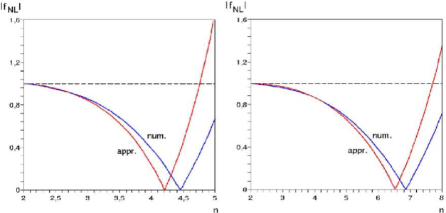
Figure 1: The qualitative behaviour of the non-linearity parameter with $s=0.2$ on the left panel and $s=0.05$ on the right panel; the values of $|f_{NL}|$ are in units $5/3r=1$. Apart from the analytical result of Eq. (17) we also show a numerical result obtained directly from Eqs. (7), (8) setting $t=1/m_{\sigma}$ as the beginning of the oscillations.

The value of the non-linearity parameter depends on the parameters $\lambda,\sigma_{*},m_{\sigma}$, but nevertheless Fig. 1 reveals the generic qualitative behaviour of $|f_{NL}|$ as $n$ is varied. One can clearly see that when the exponent of the potential correction is increased, the amount of the non-Gaussianity first begins to decrease as compared to the quadratic case. However, at large $n$ the value of $|f_{NL}|$ begins to grow rapidly.

The explanation for the behaviour of $|f_{NL}|$ and the physics involved is most transparent if we switch to the perturbative point of view. Using perturbation theory one finds [11, 19] that the $1/r$ part in Eq. (7) represents the first order contribution while the rest is due to second order effects. Thus the first order theory is adequate as long as we restrict ourselves in the region where the $1/r$ term dominates. The decrease in the amount of the non-Gaussianity means that the perturbations become smaller compared to the background value. In our case this would imply that after inflation the perturbations are damped faster than the background value. Indeed, we see that this is the case by considering the first order equation of motion for the perturbations, $\delta\ddot{\sigma}+\frac{3}{2t}\delta\dot{\sigma}+V^{\prime\prime}(\sigma)\delta\sigma=0$, with a potential correction of the form $\lambda m_{\sigma}^{4-n}\sigma^{n}$. If the potential is purely quadratic the perturbations and the background field apparently obey the same equation.

The increase of the exponent $n$ diminishes the energy density of the background field at the beginning of oscillations since we are keeping $s$ fixed. Furthermore, the energy density associated with the perturbations at the end of inflation gets bigger. With a large enough $n$ these effects become dominant over the damping of the perturbations whence the amount of non-Gaussianity again begins to grow. From Fig. 1 we see that the bigger the value of $s$, the smaller is the value of $n$ at which the growth begins; this is of course quite reasonable.

We should point out here that the increase in $|f_{NL}|$ with a large $n$ typically happens when the potential correction becomes significant, $s\sim{2}/{n}$. At this point the perturbative approach breaks down and the result (Eq. (17)) can be at most in a qualitative agreement with the true behaviour of $f_{NL}$. The drastic increase in the value of $|f_{NL}|$ seen in Fig. 1 is partly due to this effect. In Fig. 1 we also display the result of a numerical analysis in which we have, for simplicity, neglected the small change in the time $t_{\rm osc}$ corresponding to the beginning of oscillations. The values of $|f_{NL}|$ thus obtained are not significantly different from the perturbative results which is to be expected since only the region $s\lesssim{2}/{n}$ is shown in Fig. 1. The increase in $|f_{NL}|$ levels out, however.

When the correction $s$ becomes even larger $s\gtrsim{2}/{n}$ one no longer can ignore the effect on the beginning of oscillations. Indeed, the perturbations begin to oscillate way before the background field and the oscillation may not initially take place in the quadratic part of potential. We do not consider such large corrections in detail here but we make some general remarks on the behaviour of $f_{NL}$ justifying the use of the perturbative results in the region $s\sim{2}/{n}$ and giving a qualitative understanding of the region $s\gtrsim{2}/{n}$ not covered by our perturbative treatment. Using Eq. (8) we find that the condition for a local extremum in $f_{NL}(n)$ can approximatively be written as

$$\sigma_{\rm osc}\sigma_{\rm osc}^{\prime\prime} = {\sigma^{\prime}}_{\rm osc}^{2}+\frac{1}{m_{\sigma}^{2}}\Big{(}\sigma_{\rm osc}\partial_{n}\ddot{\sigma}_{\rm osc}^{\prime\prime}+\sigma_{\rm osc}^{\prime\prime}\partial_{n}\ddot{\sigma}_{\rm osc}-2\frac{\sigma_{\rm osc}\sigma_{\rm osc}^{\prime\prime}}{\sigma_{\rm osc}^{\prime}}\partial_{n}\ddot{\sigma}^{\prime}\Big{)}.$$ (19)

To obtain this result we have assumed the potential correction to be of the same order of magnitude as the quadratic part. In the limit of small corrections $\lambda\ll 1$ the expression in parenthesis in Eq. (19) vanishes and, since $\sigma^{\prime\prime}_{\rm osc}<0$ by Eq. (16), we see that in this region $f_{NL}$ is a monotonously decreasing function of $n$; this is consistent with our perturbative result Eq. (17). However, when the correction becomes larger the terms in Eq. (19) involving time derivatives are no longer negligible. Thus, for certain values of $n$ there exist solutions to Eq (19) implying that the growth of the non-linearity parameter $|f_{NL}|$ in the region $s\gtrsim{2}/{n}$ eventually ceases whereafter $|f_{NL}|$ begins to oscillate. We do not examine the non-Gaussianity in this region more closely but we point out that $|f_{NL}|$ might become large enough to exclude some classes of potentials already with the present WMAP limits [3].

5 Restrictions on the potential correction

So far we have considered the potential corrections only from a technical point of view. There are, however, some physical motivations for choosing non-quadratic potential. Small corrections of the type $n=2+\epsilon$ typically represent the effects coming from one-loop corrections due to light degrees of freedom the curvaton couples to. As we have seen above, these tend to decrease the amount of non-Gaussianity. Also, it is conceivable that the curvaton is self-interacting. The $n=4$ term, in particular, would be interesting since it implies less fine-tuning to satisfy the smallness condition of the correction $s\ll{2}/{n}$; for $n=4$ one would not have to require $\lambda\lll 1$ as for the higher order cases such as might arise, for example, in models [20, 21] where the curvaton field is considered to be one of the flat directions of the Minimally Supersymmetric Standard Model.

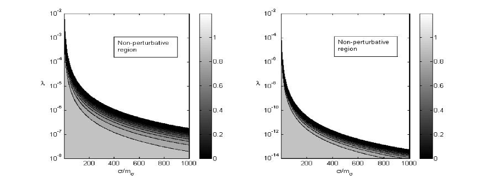
Figure 2: The non-linearity parameter $|f_{NL}|$ in units $5/3r=1$ as a contourplot with $n=4$ on the left panel and $n=6$ on the right panel. The scale on y-axis is logarithmic. The values of $|f_{NL}|$ are evaluated only in the perturbative region $s\lesssim 2/n$ and the non-perturbative region is printed in white.

This is also seen in Fig. 2 where we show $f_{NL}$ as a contourplot in $(\sigma/m_{\sigma},\lambda)$ space for $n=4$ and $n=6$. We note that especially in the $n=4$ case there is a significant region in the parameter space in which the potential correction is small $s\lesssim 2/n$ but the value of $f_{NL}$ is highly suppressed from the quadratic case. For non-renormalizable terms $(n>4)$ the requirement of negligible inflaton-generated curvature perturbations sets an upper limit on $\lambda$ (e.g. for n=6 $\lambda\lesssim 10^{-10}$), but the region in the parameter space with small values of $|f_{NL}|$ is still considerable. In other words, it is quite possible to obtain $|f_{NL}|\ll 1$ even in the curvaton models by adding a small self-interaction term to the quadratic potential.

WMAP yields an upper limit [2] $|f_{NL}|\lesssim 100$, which in the case of a quadratic curvaton potential implies that $r\gtrsim 0.02$ [8] as it can be seen from Eq. (1). For the non-quadratic case, the limit is greatly modified due to the decrease in $f_{NL}$. From Eq. (17) the part of the parameter space $(s,r)$ compatible with present observations is given by

$$r>\frac{1}{60}\Big{|}1+\frac{n(n-1)(n-2)g(n)(0.41s+0.25s^{2}ng(n))}{(0.81+0.50n(n-1)sg(n))^{2}}\Big{|}.$$ (20)

The allowed region is represented in Fig. 3 for a choice of parameter values.

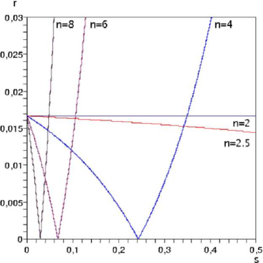
Figure 3: Allowed regions in the parameter space $(s,r)$. The labels are outside the allowed region for a given value of $n$.

It is noteworthy that the limits on $r$ are strongly dependent on the size $s$ and form $n$ of the potential correction. In the non-perturbative region not shown in Fig. 3 we expect the increase in the lower limit on $r$ to level out as a result of the behaviour of $f_{NL}$ described above.

6 Conclusions

In this paper we have examined how a small departure from the quadratic curvaton potential will affect the produced level of non-Gaussianity of the primordial curvature perturbation. For non-quadratic potentials there are two competing, opposite effects that contribute to the net non-Gaussianity. First, unlike in the quadratic case, the perturbations will be damped faster than the background value. This tends to reduce the value of the non-linearity parameter $|f_{NL}|$. Second, the increase of the exponent $n$ diminishes the energy density associated with the background field at the beginning of oscillations. With for a steep enough potential this effect becomes dominant and compensates for the damping of the perturbations. As a consequence, the value of $|f_{NL}|$ will increase as compared with the purely quadratic case.

The net outcome is that although a small departure from a quadratic curvaton potential does not modify significantly the Gaussian part of the perturbation, it can have a pronounced effect on the level of non-Gaussianity. In particular, the limit $|f_{NL}|\ll 1$ is allowed even with small curvaton energy densities $r\ll 1$. This is in sharp contrast with the quadratic result [8, 11] and shows that the curvaton models are not ruled out by a possible non-detection of non-Gaussianity as it has been suggested in e.g. [8]. Furthermore, unlike in the quadratic case, there are no strict limits that could be placed on the curvaton energy density parameter $r$. By adding a small correction to the potential, in practice one can enable arbitrarily small $r$ with suitably chosen parameter values. This is an interesting result in the sense that it implies that one can not use present observations to fix the lower limit for the energy scale of an approximately quadratic curvaton potential without making further assumptions about the higher order terms.

- [1] N. Bartolo, E. Komatsu, S. Matarrese and A. Riotto, Non-Gaussianity from inflation: Theory and observations, Phys. Rept. 402 (2004) 103 [arXiv:astro-ph/0406398].
- [2] E. Komatsu et al., First Year Wilkinson Microwave Anisotropy Probe (WMAP) Observations: Tests of Gaussianity, Astrophys. J. Suppl. 148 (2003) 119 [arXiv:astro-ph/0302223].
- [3] D. Babich and M. Zaldarriaga, Primordial Bispectrum Information from CMB Polarization, Phys. Rev. D 70 (2004) 083005 [arXiv:astro-ph/0408455].
- [4] J. Maldacena, Non-Gaussian features of primordial fluctuations in single field inflationary models, JHEP 0305 (2003) 013 [arXiv:astro-ph/0210603].
- [5] K. Enqvist and M. S. Sloth, Adiabatic CMB perturbations in pre big bang string cosmology, Nucl. Phys. B 626 (2002) 395 [arXiv:hep-ph/0109214].
- [6] T. Moroi and T. Takahashi, Effects of cosmological moduli fields on cosmic microwave background, Phys. Lett. B 522 (2001) 215 [Erratum-ibid. B 539 (2002) 303] [arXiv:hep-ph/0110096].
- [7] D. H. Lyth and D. Wands, Generating the curvature perturbation without an inflaton, Phys. Lett. B 524 (2002) 5 [arXiv:hep-ph/0110002].
- [8] D. H. Lyth and Y. Rodriguez, Non-gaussianity from the second-order cosmological perturbation, Phys. Rev. D 71 (2005) 123508 [arXiv:astro-ph/0502578].
- [9] N. Bartolo and A. R. Liddle, The simplest curvaton model, Phys. Rev. D 65 (2002) 121301 [arXiv:astro-ph/0203076].
- [10] D. H. Lyth and Y. Rodriguez, The inflationary prediction for primordial non-gaussianity, arXiv:astro-ph/0504045.
- [11] N. Bartolo, S. Matarrese and A. Riotto, On non-Gaussianity in the curvaton scenario, Phys. Rev. D 69 (2004) 043503 [arXiv:hep-ph/0309033].
- [12] M. Sasaki and E. D. Stewart, A General analytic formula for the spectral index of the density perturbations produced during inflation, Prog. Theor. Phys. 95 (1996) 71 [arXiv:astro-ph/9507001].
- [13] D. Wands, K. A. Malik, D. H. Lyth and A. R. Liddle, A new approach to the evolution of cosmological perturbations on large scales, Phys. Rev. D 62 (2000) 043527 [arXiv:astro-ph/0003278].
- [14] D. H. Lyth, K. A. Malik and M. Sasaki, A general proof of the conservation of the curvature perturbation, JCAP 0505 (2005) 004 [arXiv:astro-ph/0411220].
- [15] V. F. Mukhanov, H. A. Feldman and R. H. Brandenberger, Theory Of Cosmological Perturbations. Part 1. Classical Perturbations. Part 2. Quantum Theory Of Perturbations. Part 3. Extensions, Phys. Rept. 215 (1992) 203.
- [16] K. A. Malik and D. Wands, Evolution of second order cosmological perturbations, Class. Quant. Grav. 21 (2004) L65 [arXiv:astro-ph/0307055].
- [17] E. Komatsu and D. N. Spergel, Acoustic signatures in the primary microwave background bispectrum, Phys. Rev. D 63 (2001) 063002 [arXiv:astro-ph/0005036].
- [18] D. H. Lyth, Can the curvaton paradigm accommodate a low inflation scale, Phys. Lett. B 579 (2004) 239 [arXiv:hep-th/0308110].
- [19] D. H. Lyth, C. Ungarelli and D. Wands, The primordial density perturbation in the curvaton scenario, Phys. Rev. D 67 (2003) 023503 [arXiv:astro-ph/0208055].
- [20] K. Enqvist, Curvatons in the minimally supersymmetric standard model, Mod. Phys. Lett. A 19, (2004) 1421 [arXiv:hep-ph/0403273].
- [21] K. Enqvist, A. Jokinen, S. Kasuya and A. Mazumdar, MSSM flat direction as a curvaton, Phys. Rev. D 68 (2003) 103507 [arXiv:hep-ph/0303165].