Electrodynamics in Friedmann-Robertson-Walker Universe: Maxwell and Dirac fields in Newman-Penrose formalism

Abstract

Maxwell and Dirac fields in Friedmann-Robertson-Walker spacetime is investigated using the Newman-Penrose method. The variables are all separable, with the angular dependence given by the spin-weighted spherical harmonics. All the radial parts reduce to the barrier penetration problem, with mostly repulsive potentials representing the centrifugal energies. Both the helicity states of the photon field see the same potential, but that of the Dirac field see different ones; one component even sees attractive potential in the open universe. The massless fields have the usual exponential time dependencies; that of the massive Dirac field is coupled to the evolution of the cosmic scale factor $a$. The case of the radiation filled flat universe is solved in terms of the Whittaker function. A formal series solution, valid in any FRW universe, is also presented. The energy density of the Maxwell field is explicitly shown to scale as $a^{-4}$. The co-moving particle number density of the massless Dirac field is found to be conserved, but that of the massive one is not. Particles flow out of certain regions, and into others, creating regions that are depleted of certain linear and angular momenta states, and others with excess. Such current of charged particles would constitute an electric current that could generate a cosmic magnetic field. In contrast, the energy density of these massive particles still scales as $a^{-4}$.

1 Introduction

The Newman-Penrose[1] formalism of projecting vectors, tensors and spinors onto a set of null tetrad bases has proved to be an immensely useful tool with which to investigate the properties of quantum fields in curved spacetime. It has been used successfully in various black hole geometries [2, 3, 4]. The method has also been used more recently[5] to further study the behaviour of Dirac particles in different geometries. As the geometry of our Universe is of the Friedmann-Robertson-Walker type, it is important to study how electrodynamics is altered by the real expanding Universe in contrast to that in Minkowskian spacetime. The behaviour of the quantum fields in FRW spacetime must be indicative of the exact nature of the geometry of our Universe, particularly whether it is flat, closed or open. Properties of matter fields in general, and the massive Dirac fields in particular, must have profound consequences on the structure formation process. Propagation of electromagnetic waves in FRW spacetime was studied by Haghighipour[6] (see references therein), among other authors.The Dirac field was studied in the NP formalism by Zecca[7] and the work was continued further by Sharif[8]. This paper is another attempt to use the NP method to study the behaviour of Maxwell and Dirac fields in the Universe. A slightly different null-tetrad bases are chosen in this paper, resulting in equations that take on the familiar barrier penetration forms without much ado. The Maxwell equations for free electromagnetic waves are exactly solvable for all cases in terms of well known special functions. The spatial part of the Dirac equations are also exactly solvable; the time evolution however is coupled to the evolution of the scale factor, can be solved in terms of known functions only for the case of a radiation dominated universe.

The FRW line element is usually written in the comoving coordinates as[9]

$$ds^{2}=dt^{2}-a^{2}(t)\left(\frac{dr^{\prime 2}}{1-Kr^{\prime 2}}+r^{\prime 2}\left(d\theta^{2}+\sin^{2}\theta d\phi^{2}\right)\right),$$ (1)

where $a(t)$ is the scale factor; the curvature constant $K$ can be scaled to the values $0,+1$ or $-1$ to describe the flat, closed or open universe respectively. In terms of the conformal time $\eta=\int\frac{dt}{a}$, and a change of variable $r^{\prime}=r/\left(1+Kr^{2}/4\right)=r/f(r)$, the line element Eq. (1) becomes[10]

$$ds^{2}=a^{2}(\eta)\left[d\eta^{2}-\frac{1}{f^{2}(r)}\left(dr^{2}+r^{2}\left(d\theta^{2}+\sin^{2}\theta d\varphi^{2}\right)\right)\right].$$ (2)

Following Chandrasekhar’s guidelines for the black hole[11], we can introduce the null tetrad $l_{\mu}=\left(1,-\frac{1}{f},0,0\right),n_{\mu}=\frac{a^{2}}{2}\left(1,\frac{1}{f},0,0\right),m_{\mu}=\frac{ar}{\sqrt{2}f}\left(0,0,-1,-i\sin\theta\right)$, and the complex conjugate $m_{\mu}^{\ast}$ . The non vanishing spin-coefficients are $\beta=-\alpha=\frac{f}{2\sqrt{2}ar}\cot\theta,\rho=-\frac{f}{a^{2}}\left(\frac{\dot{a}}{af}-\frac{\left(f/r\right)^{\prime}}{f/r}\right),\mu=\frac{f}{2}\left(\frac{\dot{a}}{af}+\frac{\left(f/r\right)^{\prime}}{f/r}\right)$, and $\gamma=-\frac{\dot{a}}{2a},$where the prime and the overdot denote derivatives with respect to $r$ and $\eta$ respectively.

Besides the vanishing of the spin-coefficient $\kappa$ because the $l$ vector forms a congruence of null geodesics, and of $\pi$ telling us that the tetrad bases remain unchanged as they are parallely propagated along $l$ as in Ref.[7], the present choice of the bases are affinely parameterized so that $\varepsilon$ also vanishes. The directional derivatives can then be written down as $D=l^{\mu}\partial_{\mu}=\frac{1}{a^{2}}D_{-},\Delta=n^{\mu}\partial_{\mu}=-\frac{1}{2}D_{+},$ $\delta=m^{\mu}\partial_{\mu}=\frac{f}{\sqrt{2}ar}L_{-},$ and $\delta^{\ast}=m^{\ast\mu}\partial_{\mu}=\frac{f}{\sqrt{2}ar}L_{+},$where $D_{\pm}=f\frac{\partial}{\partial r}\mp\frac{\partial}{\partial\eta}$and $L_{\pm}=\frac{\partial}{\partial\theta}\mp\frac{i}{\sin\theta}\frac{\partial}{\partial\varphi}$. In terms of what may be called the “tortoise” coordinate defined by

$$r_{\ast}=\int\frac{dr}{f}=\frac{2}{\sqrt{K}}\text{arctan}\frac{\sqrt{K}r}{2}=\left\{\begin{array}[]{cc}r,&K=0\\ 2\,\text{arctan}(r/2),&K=1\\ 2\,\text{arctanh}(r/2),&K=-1\end{array}\right.,$$ (3)

$D_{\pm}=\frac{\partial}{\partial r_{\ast}}\mp\frac{\partial}{\partial\eta}$. The tortoise coordinate shown in Fig. 1 reveals that, near the origin all the $r_{\ast}$’s coincide with each other; also, from Eq. (3) it is seen that as $r\rightarrow 0,r_{\ast}\rightarrow r$ for both $K=\pm 1$; thus, at small distances both the closed and open universes look basically flat.

The Maxwellian wave equations are solved in the next Section, and the solutions are used to investigate the behaviour of the energy-momentum in the expanding Universe. Section 3 is devoted to Dirac equations; the spatial parts of the four components are easily solved, and so is the time dependence of the massless field; the time dependence of the massive field is more complicated as it is coupled to the evolution of $a$; nonetheless, the case of the radiation filled flat universe is found to have a solution in terms of the Whittaker function. A formal series solution that can be used in any FRW universe is also written down. The behaviour of the Dirac current and energy-momentum is then investigated. The final Section makes some concluding remarks.

2 Maxwell Field

In the NP formalism, the six independent components of the antisymmetric Maxwell tensor $F_{\mu\nu}$ are replaced by the three complex scalars[11] $\Phi_{0}=F_{\mu\nu}l^{\mu}m^{\nu},\ \Phi_{1}=\frac{1}{2}F_{\mu\nu}\left(l^{\mu}n^{\nu}+m^{\ast\mu}m^{\nu}\right),\,\Phi_{2}=F_{\mu\nu}m^{\ast\mu}n^{\nu}$. Then the Maxwell equations become

$$\left(D-2\rho\right)\Phi_{1} = \left(\delta^{\ast}+\pi-2\alpha\right)\Phi_{0}-\kappa\Phi_{2},$$

$$\left(\delta-2\tau\right)\Phi_{1} = \left(\Delta+\mu-2\gamma\right)\Phi_{0}-\sigma\Phi_{2},$$

$$\left(D-\rho+2\varepsilon\right)\Phi_{2} = \left(\delta^{\ast}+2\pi\right)\Phi_{1}-\lambda\Phi_{0}\,\text{and}$$

$$\left(\delta-\tau+2\beta\right)\Phi_{2} = \left(\Delta+2\mu\right)\Phi_{1}-\nu\Phi_{0}.$$ (4)

With the spin-coefficients and the directional derivatives from Sec. 1, and using the fact that $(1/f)D_{\pm}\left[a^{n}(f/r)^{m}\Phi\right]=a^{n}(f/r)^{m}\left(\frac{1}{f}D_{\pm}\mp\,\frac{n\dot{a}}{af}+m\frac{\left(f/r\right)^{\prime}}{\left(f/r\right)}\right),$ Eqs. (4) become

$$D_{-}\left[\sqrt{2}\Phi_{1}\left(\frac{ar}{f}\right)^{2}\right] = \left(L_{+}+\cot\theta\right)\left[\Phi_{0}\frac{ra^{3}}{f}\right],$$

$$L_{-}\left[\sqrt{2}\Phi_{1}\left(\frac{ar}{f}\right)^{2}\right] = -\frac{r^{2}}{f^{2}}D_{+}\left[\Phi_{0}\frac{ra^{3}}{f}\right],$$

$$\frac{r^{2}}{f^{2}}D_{-}\left[\frac{2ar}{f}\Phi_{2}\right] = L_{+}\left[\sqrt{2}\Phi_{1}\left(\frac{ra}{f}\right)^{2}\right]\,\text{and}$$

$$\left(L_{-}+\cot\theta\right)\left[\frac{2ar}{f}\Phi_{2}\right] = -D_{+}\left[\sqrt{2}\Phi_{1}\left(\frac{ra}{f}\right)^{2}\right].$$ (5)

The first of the two pairs of Eqs. (5) can be used together to eliminate $\Phi_{1}$ and be combined into a second order equation for $\Phi_{0}$ only, and similarly from the second pair for the equation for $\Phi_{2}$ only. Writing $\Phi_{+}=\Phi_{0}ra^{3}/f$ and $\Phi_{-}=2\Phi_{2}ar/f,$the resulting two equations take the form

$$D_{\mp}\left[\frac{r^{2}}{f^{2}}D_{\pm}\Phi_{\pm}\right]+L_{\mp}\left[L_{\pm}+\cot\theta\right]\Phi_{\pm}=0.$$ (6)

It is clear that the Maxwell scalars in Eq. (6) are separable into $\Phi_{\pm}=\phi_{\pm}(r,\eta)Y_{\pm 1}(\theta,\varphi)$. Then the angular parts become

$$\left(\frac{1}{\sin\theta}\frac{\partial}{\partial\theta}\sin\theta\frac{\partial}{\partial\theta}\pm\frac{2i\cos\theta}{\sin^{2}\theta}\frac{\partial}{\partial\varphi}+\frac{1}{\sin^{2}\theta}\frac{\partial^{2}}{\partial\varphi^{2}}-\cot^{2}\theta-1\right)Y_{\pm 1}=-\lambda Y_{\pm 1},$$ (7)

where $\lambda$ is the separation constant. Same eigenvalue $\lambda$ is used for both the solutions $Y_{\pm 1}$because the equation for $Y_{+1}$ goes over to that for $Y_{-1}$ with the change of variable $\theta\rightarrow\pi-\theta;$ the two just represent the two helicity states of the photon. The solutions are the spin weighted spherical harmonics of Goldberg, et al. [12] with $\lambda=l(l+1);$ $l$ is the total angular momentum of the field including its spin, so in this case for photons, $l=1,2,3,...$. It is obvious that the azimuthal part is just $e^{im\varphi}$. The radial and time parts then become

$$D_{\mp}\left[\frac{r^{2}}{f^{2}}D_{\pm}\phi_{\pm}\right]=\lambda\phi_{\pm}.$$ (8)

The relative normalization between the two helicity states is set by the easily verifiable Teukolsky type relations

$$D_{\pm}\left[\frac{r^{2}}{f^{2}}D_{\pm}\phi_{\pm}\right]=\lambda\phi_{\mp}.$$ (9)

Substituting $Z=$ $\frac{r^{2}}{f^{2}}D_{\pm}\phi_{\pm}$ for the dependent variable in Eq. (8), operating on it with $D_{\pm}$, and writing $D^{2}=D_{\pm}D_{\mp}=\frac{\partial^{2}}{\partial r_{\ast}^{2}}-\frac{\partial^{2}}{\partial\eta^{2}},$ we end up with the equation of motion$D^{2}Z=VZ,$ with the potential $V=\lambda(f/r)^{2}$ independent of $\eta$. Consequently, the time dependence $e^{-i\omega\eta}$ can be factored out. For the stipulated time and azimuthal dependence, $D_{\pm}=\frac{\partial}{\partial r_{\ast}}\pm i\omega$ and $L_{\pm}=\frac{\partial}{\partial\theta}\pm\frac{m}{\sin\theta}$. Then the radial parts of $\phi_{\pm}$, which may be written as $R_{\pm}$ in Eq. (8), satisfy complex conjugate equations. Finally, we are left with the equation for the radial dependence of $Z$ as,

$$\left[\frac{d^{2}}{dr_{\ast}^{2}}+\omega^{2}\right]R=VR,$$ (10)

which has taken the familiar form of the one dimensional quantum mechanical barrier penetration problem with the potentials for the three cases given by

$$V=\left\{\begin{array}[]{cc}l(l+1)/r^{2},&K=0\\ l(l+1)/\sin^{2}r_{\ast},&K=1\\ l(l+1)/\sinh^{2}r_{\ast},&K=-1\end{array}\right..$$ (11)

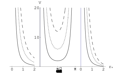
Figure 2: The potential seen by electromagnetic waves. $l=1,2$, and $3$, for the solid, dotted and dashed lines. $K=0,1$, and $-1$ from left to right. The potential is a $1/r^{2}$ wall in the first, become infinitely high wall at each boundary in the second, and an exponentially decaying wall in the third case. The walls are thicker for higher $l$.

Eq. (10) is basically the same as that derived in Ref.[6]. The potentials barriers represented by Eq. (11) are just the rotational kinetic energies. They become thicker for larger $l$. The barriers go down as $1/r^{2}$ in the flat universe, fall off even more rapidly in the open universe, and are potential wells between $0<$ $r_{\ast}<\pi$ that rise to infinity towards both the ends in the closed universe (Fig. 2). If $r_{\ast}$ is replaced by $ir_{\ast}$ and $\omega$ by $i\omega$ in the potential for $K=1$ in Eq. (11) we end up with the one for $K=-1$. Both the spin states of the photon satisfy the same equation with the same real potential. The inversion relation is provided by the normalization condition Eq. (9) as

$$\lambda R_{\pm}=D_{\mp}R.$$ (12)

2.1 Solutions

All the three cases of Eq. (10) can fortunately be solved. For $K=1$, $f(r)=1\,$and $r_{\ast}=r$. Then Eq. (10) has the general solution [13]

$$R=r\left[A_{0}j_{l}\left(\omega r\right)+B_{0}y_{l}\left(\omega r\right)\right],$$ (13)

where $j_{l}$ and $y_{l}$ are the respective spherical Bessel functions. As $l\geq 1$, only the $j$’s are regular at the origin. In the asymptotic region, as $2j_{l}=h_{l}^{(1)}+h_{l}^{(2)}\rightarrow\left[(-i)^{l+1}e^{i\omega r}+(i)^{l+1}e^{-i\omega r}\right]/\omega$, we can use the inversion relation Eq. (12) to see that the incoming waves are dominated by $R_{+}$and the outgoing by $R_{-}$.

In the closed universe, it is most convenient to write the solutions in terms of the Gegenbauer functions $C_{n}^{\alpha}$ as

$$R=A_{1}\left(\sin r_{\ast}\right)^{l+1}C_{\omega-l-1}^{l+1}\left(\cos r_{\ast}\right)+B_{1}\left(\sin r_{\ast}\right)^{-l}C_{\omega+l}^{-l}\left(\cos r_{\ast}\right).$$ (14)

Again, the first one is regular within the allowed range of $r_{\ast}$, and $\omega\geq l+1$. These em waves form standing waves.

We may write the solution in the open universe as

$$R = A_{-1}e^{i\omega r_{\ast}}\,_{2}F_{1}\left(-l,l+1,1-i\omega,\frac{1}{2}(1-\coth r_{\ast})\right)$$ (15)

$$+B_{-1}e^{-i\omega r_{\ast}}\,_{2}F_{1}\left(-l,l+1,1+i\omega,\frac{1}{2}(1-\coth r_{\ast})\right),$$

consisting of the outgoing and incoming parts at $r_{\ast}\rightarrow\infty$. Alternatively, we may make the replacements $r_{\ast}\rightarrow ir_{\ast}$ and $\omega\rightarrow i\omega$ in Eq. (14) to study the behaviour near the origin. Once $\Phi_{0}$ and $\Phi_{2}$ are known, Eq. (4) can be used to determine $\Phi_{1}$ and complete the solutions for the electromagnetic field.

2.2 Energy Momentum

The energy-momentum tensor of the Maxwell field in terms of the $\Phi$’s is given by

$$4\pi T_{\alpha\beta} = \left|\Phi_{0}\right|^{2}n_{\alpha}n_{\beta}+\left|\Phi_{2}\right|^{2}l_{\alpha}l_{\beta}+2\left|\Phi_{1}\right|^{2}\left\{l_{(\alpha}n_{\beta)}+m_{(\alpha}m_{\beta)}^{\ast}\right\}$$ (16)

$$-4\Phi_{0}^{\ast}\Phi_{1}n_{(\alpha}m_{\beta)}-4\Phi_{1}^{\ast}\Phi_{2}l_{(\alpha}m_{\beta)}+2\Phi_{0}^{\ast}\Phi_{2}m_{(\alpha}m_{\beta)}+\text{cc,}$$

where the brackets around the indices of the null-tetrad denote symmetrization and cc is the complex conjugates of preceeding terms; $T_{\alpha\beta}$ is obviously traceless. We are particularly interested in the time components which can be determined as

$$4\pi\rho = 4\pi T_{\eta}^{\eta}=\frac{f^{2}}{2r^{2}a^{4}}\left[\left|\Phi_{+}\right|^{2}+\left|\Phi_{-}\right|^{2}\right]+2\left|\Phi_{1}\right|^{2}$$

$$= -4\pi\left(T_{r}^{r}+T_{\theta}^{\theta}+T_{\varphi}^{\varphi}\right)$$

$$4\pi T_{\eta}^{r} = -\frac{f^{3}}{2r^{2}a^{4}}\left[\left|\Phi_{+}\right|^{2}-\left|\Phi_{-}\right|^{2}\right],$$ (17)

where $\rho$ is the energy density. The $\theta$ and $\varphi$ components are not important for our analysis. Noting that the necessary non-vanishing Christoffel symbols are $\Gamma_{\eta\eta}^{\eta}=\Gamma_{r\eta}^{r}=\Gamma_{\theta\eta}^{\theta}=\Gamma_{\varphi\eta}^{\varphi}=\dot{a}/a$ where the overdot represents derivative with respect to $\eta$, we may write the conservation equation as $\partial_{\eta}\left(\sqrt{g}T_{\eta}^{\eta}\right)=-\partial_{i}\left(\sqrt{g}T_{\eta}^{i}\right)$, where $g=-\det g_{\alpha\beta}=\left(\frac{a^{4}r^{2}}{f^{3}}\sin\theta\right)^{2}=a^{8}g_{3}$ where $g_{3}$ is the determinant of the 3-space; the terms with the $\Gamma$’s are not written as their sum vanish due to the tracelessness. Integrating over the three space we find

$$\partial_{\eta}\left(Ea^{4}\right)=-a^{4}\int\partial_{i}\left(\sqrt{g_{3}}T_{\eta}^{i}\right)=-a^{4}\int d\Sigma_{r}T_{\eta}^{r}=a^{4}\int d\Sigma_{r}\frac{f^{3}}{r^{2}}\left(\left|\Phi_{+}\right|^{2}-\left|\Phi_{-}\right|^{2}\right),$$ (18)

where $E$ is the total energy contained within a spherical volume of radius $r$, and $d\Sigma_{r}=\frac{r^{2}}{f^{3}}\sin\theta d\theta d\varphi$ is an elemental area normal to the radial direction. Using the inversion relation, Eq. (12), we get $\lambda^{2}\left[\left|\Phi_{+}\right|^{2}-\left|\Phi_{-}\right|^{2}\right]=\left[\left|D_{-}Z\right|^{2}\left|Y_{+}\right|^{2}-\left|D_{+}Z\right|^{2}\left|Y_{-}\right|^{2}\right]=\left[\left|\frac{dR}{dr_{\ast}}\right|^{2}+\omega^{2}\left|R\right|^{2}\right]\left(\left|Y_{+}\right|^{2}-\left|Y_{-}\right|^{2}\right)$$+i\omega W[R^{\ast},R]\left(\left|Y_{+}\right|^{2}+\left|Y_{-}\right|^{2}\right)$, where $W$ is the Wronskian. As the $Y$’ s are normalized to unity, when we perform the angular integration, the first term on the left hand side will vanish. Now $R$ and $R^{\ast}$ satisfy the same equation and are proportional to the same function so that the Wronskian will also vanish.Hence $Ea^{4}$ remains constant, and so does $\rho a^{4}$, during the evolution of the Universe. As a consequence, there is no net flux of electromagnetic energy flowing out of a closed surface. This is a direct proof of the well known result that the energy density of massless radiation scales as $a^{-4}$.

3 Dirac Field

In NP formalism, the four components of the Dirac spinor field of mass $M$ are represented by the four functions $P^{0},P^{1},$ $-\bar{Q}^{0^{\prime}}$ and $\bar{Q}^{1^{\prime}}$ that satisfy the following Dirac equations[11]:

$$\left(D+\varepsilon-\rho\right)P^{0}+\left(\delta^{\ast}+\pi-\alpha\right)P^{1} = \frac{iM}{\sqrt{2}}\bar{Q}^{1^{\prime}},$$

$$\left(\Delta+\mu-\gamma\right)P^{1}+\left(\delta+\beta-\tau\right)P^{0} = -\frac{iM}{\sqrt{2}}\bar{Q}^{0^{\prime}},$$

$$\left(D+\varepsilon^{\ast}-\rho^{\ast}\right)\bar{Q}^{0^{\prime}}+\left(\delta+\pi^{\ast}-\alpha^{\ast}\right)\bar{Q}^{1^{\prime}} = -\frac{iM}{\sqrt{2}}P^{1},\,\text{and}$$

$$\left(\Delta+\mu^{\ast}-\gamma^{\ast}\right)\bar{Q}^{1^{\prime}}+\left(\delta^{\ast}+\beta^{\ast}-\tau^{\ast}\right)\bar{Q}^{0^{\prime}} = \frac{iM}{\sqrt{2}}P^{0}.$$ (19)

Substituting $\left(\frac{\sqrt{2}ra}{f}P^{0},\frac{ra^{2}}{f}P^{1},-\frac{\sqrt{2}ra}{f}\bar{Q}^{0^{\prime}},\frac{ra^{2}}{f}\bar{Q}^{1^{\prime}}\right)$ with $\left(\Phi_{-1/2}Y_{-1/2},\Phi_{1/2}Y_{1/2},\Phi_{-1/2}Y_{1/2},\Phi_{1/2}Y_{-1/2}\right)$, using the directional derivatives and spin-coefficients given in Sec. 1, and following similar techniques, the angular parts of Eqs. (19) are found to separate into

$$\left(L_{\pm}+\frac{1}{2}\cot\theta\right)Y_{\pm 1/2}=\mp\lambda Y_{\mp 1/2},$$ (20)

while the radial and time parts satisfy

$$rD_{\pm}\Phi_{\pm 1/2}=\left(f\lambda\mp iMra\right)\Phi_{\mp 1/2}.$$ (21)

Substituting for $Y_{+1/2}=\left(L_{-}+\frac{1}{2}\cot\theta\right)Y_{-1/2}$ from Eq. (20) into the one for $Y_{-1/2}$, and a similar process with $Y_{-1/2}$, gives us the two angular equations

$$\left(\frac{1}{\sin\theta}\frac{\partial}{\partial\theta}\sin\theta\frac{\partial}{\partial\theta}\pm\frac{i\cos\theta}{\sin^{2}\theta}\frac{\partial}{\partial\varphi}+\frac{1}{\sin^{2}\theta}\frac{\partial^{2}}{\partial\varphi^{2}}-\frac{1}{4}\cot^{2}\theta-\frac{1}{2}+\lambda^{2}\right)Y_{\pm 1/2}=0$$ (22)

where the $Y$’s are the appropriate spin weighted spherical harmonics, and the eigenvalue can be identified as $\lambda=(l+1/2);$ $l$  is again the total angular momentum including the spin, i.e., $l=n+1/2$, where $n=0,1,2,3...$. The radial and time parts of Eq. (21) can be separated with the substitution $Z_{\pm}=\Phi_{+1/2}\pm\Phi_{-1/2}=R_{\pm}T_{\pm}$ to give

$$\frac{1}{R_{\mp}}\left(\frac{\partial}{\partial r_{\ast}}\mp\lambda\frac{f}{r}\right)R_{\pm}=\frac{1}{T_{\pm}}\left(\frac{\partial}{\partial\eta}\pm iMa\right)T_{\mp}=ik,$$ (23)

whence the separation constant $k=pa$ may be identified with the co-moving momentum. The coupled first order equations in Eq. (23) can be combined into pairs of second order equations

$$\left(\frac{\partial}{\partial r_{\ast}}\pm\lambda\frac{f}{r}\right)\left(\frac{\partial}{\partial r_{\ast}}\mp\lambda\frac{f}{r}\right)R_{\pm}=\left(\frac{\partial}{\partial\eta}\pm iMa\right)\left(\frac{\partial}{\partial\eta}\mp iMa\right)T_{\pm}=-k^{2}Z_{\pm}.$$ (24)

3.1 Radial Solutions

The radial parts take the form of the barrier penetration problem

$$\left[\frac{d^{2}}{dr_{\ast}^{2}}+k^{2}\right]R_{\pm}=V_{\pm}R_{\pm},\text{ }$$ (25)

where the potentials are

$$V_{\pm}=\lambda^{2}\frac{f^{2}}{r^{2}}\pm\lambda\frac{d}{dr_{\ast}}\left(\frac{f}{r}\right).$$ (26)

Explicitly, the potentials in the three cases are

$$V_{\pm}=(l+1/2)\times\left\{\begin{array}[]{cc}(l+1/2\mp 1)/r^{2},&K=0\\ (l+1/2\mp\cos r_{\ast})/\sin^{2}r_{\ast},&K=1\\ (l+1/2\mp\cosh r_{\ast})/\sinh^{2}r_{\ast},&K=-1\end{array}\right..$$ (27)

In contrast to the case of the electromagnetic field, the two spin states of the Dirac field see different potentials. These potentials are shown in Fig. 3. In the flat FRW universe, the potential barriers basically go down as $1/r^{2}$, but $V_{+}$ is seen to vanish for $l=1/2$; this lowest spin state behaves as a free field as far as the radial co-ordinate is concerned. In the closed universe, the potentials are again infinite wells; for $l=1/2$ however, $V_{+}$ flattens out towards the origin and $V_{-}$ towards $\pi$, reaching the limiting value of $1/2$ at the respective ends. The potential in the open universe is even more interesting; $V_{+}$ is negative throughout for $l=1/2$, reaching the minimum of $-1/2$ at the origin and approaching $0$ from below for large $r_{\ast}$; even for large $l,\,V_{+}$ goes down rapidly from $\infty$ at the origin, becomes negative from $\cosh r_{\ast}>(l+1/2),$ reaches the minimum of $V_{+\min}=$ $-\frac{1}{2}(l+1/2)\left(l+1/2-\sqrt{(l-1/2)(l+3/2)}\right)$ at $\cosh r_{\ast}=(l+1/2)+$ $\sqrt{(l-1/2)(l+3/2)}$ , and then rises up to zero from below as $r_{\ast}\rightarrow\infty$; the Dirac fields of different $l$ in the open universe see the attractive potential $V_{+}$ with location of the minimum at different $r_{\ast}$ for different $l$. The radial equations turn out to be solvable for all the three cases ($K=0,\pm 1$), and the behaviour of the radial part is the same for both the massive and massless fields.In the flat universe with $K=0,$ Eq. (25) has the solutions

$$R_{\pm}=r\left[A_{1/2}j_{l\mp 1/2}(kr)+B_{1/2}y_{l\mp 1/2}(kr)\right]\text{ }.$$ (28)

For regular solution at the origin, we would choose the $j$’s, some modes of which are illustrated in Fig. 4. In the closed Universe, the radial equations are easily recognized as that for the Jacobi $P_{\nu}^{\left(\alpha,\beta\right)}$ functions. Thus, the solutions that are regular between $0\leq r_{\ast}\leq\pi$ can most conveniently be written as

$$R_{\pm}=C_{1/2}\sin^{l}r_{\ast}\left(\cot\frac{r_{\ast}}{2}\right)^{\pm 1/2}P_{k-l-1}^{\left(l+1/2\mp 1/2,l+1/2\pm 1/2\right)}(\cos r_{\ast}).$$ (29)

Some typical behaviour are shown in Fig. 4. The solution in the open universe that are just the replacements $k\rightarrow ik$ and $r_{\ast}\rightarrow ir_{\ast}$ in Eq. (29), are also shown in Fig. 4.

3.2 Time Dependence

The time dependence of the Dirac field is determined by the equation

$$\left[\frac{d^{2}}{d\eta^{2}}+k^{2}\right]T_{\pm}=V_{T\pm}T_{\pm},$$ (30)

which corresponds to a classical oscillator in a complex time potential

$$V_{T\pm}=-M^{2}a^{2}\pm iM\dot{a}.$$ (31)

The mass that has coupled with the scale factor becomes dominating at large $a$. The behaviour of the solution is controlled by the evolution of the scale factor, viz., the Friedmann equation. Friedmann equation for a universe filled with radiation, massive particles and also posessing a cosmological constant can be written as

$$\dot{a}^{2}=\Omega_{\Lambda}a^{4}+\left(1-\Omega_{M}-\Omega_{R}-\Omega_{\Lambda}\right)a^{2}+\Omega_{M}\sqrt{\left(1-v^{2}\right)a^{2}+v^{2}}+\Omega_{R},$$ (32)

where an overall factor of $H_{0}^{2}$ on the right hand side has been set equal to unity so that $\eta$ is in units of Hubble time; $\Omega_{R,M,\Lambda}$ are the respective radiation, matter and vacuum densities in units of the critical density $\rho_{c}$, and $v$ is the rms speed of the matter particles, all at a reference conformal time $\eta_{0}$ when the scale factor $a=a_{0}=1$; as before, the overdot denotes derivative with respect to $\eta$. In this paper, we will concern ourselves with $\Omega_{\Lambda}=0$. In the form in which we have written the Friedmann equation, we may as well set $\Omega_{R}=0$ and consider only $\Omega_{M}$; then $v=1$ corresponds to radiation, $v=0$ is dusty matter of zero pressure, and $0<v<1$ for any real matter of finite mass; this is how $V_{T}$ are displayed in Fig. 5 for the three cases of $\Omega_{0}=1$ (flat), $\Omega_{0}>1$ (closed), and $\Omega_{0}<1$ (open) universes. For the massless field, $V_{T}=0,$ and the time dependence is the usual $e^{-ik\eta}$. In terms of the time marker $a$ rather than $\eta$, Eq. ( 30) reads as

$$\left[\dot{a}^{2}\frac{d^{2}}{da^{2}}+\"{a}\frac{d}{da}+k^{2}+M^{2}a^{2}\mp iM\dot{a}\right]T_{\pm}=0,$$ (33)

which is in a more convenient form to tackle the massive case. Given the time evolution of $a$ by Eq. (32), we can find series or numerical solution of Eq. (33) for any general case.

Here, we present the solution, in terms of Whittaker function, in the radiation filled flat universe where $\dot{a}=1$. In contrast, Sharif[8] had to solve for the coefficients of a series solution. This may be due to the choice of different bases; the time dependence, Eq. (30), is slightly different than that of Sharif and Zecca[7]. The solution is

$$T_{+}=A_{+}e^{-iM\eta^{2}/2}U(\frac{ik^{2}}{4M}+\frac{1}{2},\frac{1}{2},iM\eta^{2})=A_{+}\frac{1}{\sqrt[4]{iM\eta^{2}}}W_{-\frac{1}{4}\left(1+\frac{ik^{2}}{m}\right),-\frac{1}{4}},$$ (34)

where $U$ and $W$ are the confluent hypergeometric and Whittaker[13] functions respectively. The logarithmic solution is chosen because it reverts to the massless behaviour $e^{-ik\eta}$ in the large $k$ limit; viz., $T_{+}\rightarrow A_{+}\sqrt{\pi}e^{-i\eta\sqrt{k^{2}-2iM}}$ as $k\rightarrow\infty$. Some typical cases of the solution are plotted in Fig. 6.

At early times, for any kind of FRW universe, we may make an expansion of the scale factor as $a\rightarrow\dot{a}_{I}\eta,$where $\dot{a}_{I}$ is the slope of $\ a$ at the big bang. From Eq. (32), we see that $\dot{a}_{I}\approx\sqrt{\Omega_{M}v+\Omega_{R}}$, and $a$ is linear in $\eta$. So the above solution, Eq. (34), is valid with the replacement $M\rightarrow M\sqrt{\Omega_{M}v+\Omega_{R}}$.

One can factor out a time dependence $T_{\pm}=e^{\pm iM(t-t_{0})}T_{1\pm}$ to write Eq. (30) in the form of a damped oscillator,

$$\frac{d^{2}T_{1\pm}}{d\eta^{2}}\pm 2iMa\frac{dT_{1\pm}}{d\eta}+k^{2}T_{1\pm}=0,$$ (35)

with a velocity dependent imaginary damping that is itself time dependent. A formal series solution of this equation, in terms of $x=\eta-\eta_{0}$ , may be written down by firstly making a Taylor expansion of the scale factor as $a\left(\eta\right)=\underset{n=0}{\overset{\infty}{\sum}}\frac{a_{n}}{n!}x^{n}$, where $a_{n}=\frac{d^{n}a\left(\eta\right)}{d\eta^{n}}|_{\eta_{0}}$. As $d\eta=dx$, Eq. (35) looks the same with $\eta\rightarrow x$. Then the series, $T_{1}=$ $\underset{n=0}{\overset{\infty}{\sum}}b_{n}x^{n}$, can be substituted in the equation to find the recursion relation

$$n(n-1)b_{n}=(-ik)^{2}b_{n-2}-(\pm 2iM)\underset{m=0}{\overset{n-2}{\sum}}\frac{a_{m}}{m!}\left(n-m-1\right)b_{n-m-1};$$ (36)

$T_{1\pm}$ will be appropriately normalized, according to the requirements that will be discussed below, with the choices $b_{\pm 0}=\pm 1/\sqrt{2}$ and $b_{\pm 1}=\mp ik/\sqrt{2}$. For $M=0$, the solution is $T_{1}=e^{-ikx}/\sqrt{2}$.

3.3 Dirac Particle Current

With the generalized form of the Pauli matrix in terms of the null-tetrad

$$\sigma_{AB^{\prime}}^{\mu}=\frac{1}{\sqrt{2}}\left(\begin{array}[]{cc}l^{\mu}&m^{\mu}\\ m^{\ast\mu}&n^{\mu}\end{array}\right),$$

and the particle current written as $\frac{1}{\sqrt{2}}J^{\mu}=\sigma_{AB^{\prime}}^{\mu}\left(P^{A}\overline{P^{A^{\prime}}}+Q^{A}\overline{Q^{B^{\prime}}}\right)$, it is easily seen that the continuity equation $\partial_{\mu}\left(\sqrt{g}J^{\mu}\right)=0$ has to be satisfied. In particular, we can calculate

$$J^{\eta} = \frac{f^{2}}{4r^{2}a^{4}}\left[\left|Z_{+}\right|^{2}+\left|Z_{-}\right|^{2}\right]\left(\left|Y_{+}\right|^{2}+\left|Y_{-}\right|^{2}\right)\text{ and}$$

$$J^{r} = -\frac{f^{3}}{4r^{2}a^{4}}\left[Z_{+}^{\ast}Z_{-}+Z_{+}Z_{-}^{\ast}\right]\left(\left|Y_{+}\right|^{2}+\left|Y_{-}\right|^{2}\right).$$ (37)

The time component of the particle current can be identified with the number density as $n=J^{t}=aJ^{\eta}$, so that $na^{3}=a^{4}J^{\eta}$ is the particle number density per unit co-moving volume. As a consequence of the Dirac equations, Eq. (23), we have on hand a number of Wronskian like conditions on the radial and time parts, of which, two useful ones are

$$\frac{d\left(R_{+}^{\ast}R_{-}\right)}{dr_{\ast}} = -\frac{d\left(R_{+}R_{-}^{\ast}\right)}{dr_{\ast}}=ik\left[\left|R_{+}\right|^{2}-\left|R_{-}\right|^{2}\right]\text{ and}$$

$$\frac{d\left|T_{+}\right|^{2}}{d\eta} = -\frac{d\left|T_{-}\right|^{2}}{d\eta}=ik\left[T_{+}^{\ast}T_{-}-T_{+}T_{-}^{\ast}\right].$$ (38)

From the first we see that $R_{+}^{\ast}R_{-}+R_{+}R_{-}^{\ast}=C_{1}$ is a real constant, which must be equal to zero as will be shown presently; hence $R_{+}^{\ast}R_{-}$ must be purely imaginary. Similarly, from the second one we find that $\left|T_{+}\right|^{2}+\left|T_{-}\right|^{2}=C_{2}$ must be a positive real constant which can be normalized to unity. Now, $\partial_{\eta}\left[\left|Z_{+}\right|^{2}+\left|Z_{-}\right|^{2}\right]=\left|R_{+}\right|^{2}\frac{d\left|T_{+}\right|^{2}}{d\eta}+\left|R_{-}\right|^{2}\frac{d\left|T_{-}\right|^{2}}{d\eta}=\left(\left|R_{+}\right|^{2}-\left|R_{-}\right|\right)\frac{d\left|T_{+}\right|^{2}}{d\eta}=\frac{1}{ik}\frac{d\left(R_{+}^{\ast}R_{-}\right)}{dr_{\ast}}\frac{d\left|T_{+}\right|^{2}}{d\eta}$. Thus, $\partial_{\eta}\sqrt{g}J^{\eta}=\sqrt{g_{3}}\partial_{\eta}\left(na^{3}\right)=\frac{1}{4ikf}\frac{d\left(R_{+}^{\ast}R_{-}\right)}{dr_{\ast}}\frac{d\left|T_{+}\right|^{2}}{d\eta}\left(\left|Y_{+}\right|^{2}+\left|Y_{-}\right|^{2}\right)$, and the particle current out of a co-moving spatial volume of radius $r$ is the integration over the spatial volume:

$$\frac{\partial\left(Na^{3}\right)}{\partial\eta}=\int_{0}^{r}drd\theta d\varphi\frac{1}{4ikf}\frac{d\left(R_{+}^{\ast}R_{-}\right)}{dr_{\ast}}\frac{d\left|T_{+}\right|^{2}}{d\eta}\left(\left|Y_{+}\right|^{2}+\left|Y_{-}\right|^{2}\right)=\frac{R_{+}^{\ast}R_{-}}{2ik}\frac{d\left|T_{+}\right|^{2}}{d\eta};$$ (39)

here, we have used the property that the product of the radial functions vanishes at the origin, and $N$ is the total number of particles remaining within the volume. Thus, the net change in the number of of particles within a co-moving volume of radius $r$ between the times $\eta_{0}$ and $\eta$ is given by $\Delta_{N}=N_{0}a_{0}^{3}-Na^{3}=\frac{R_{+}^{\ast}R_{-}}{2ik}\left[\left|T_{+}\left(\eta_{0}\right)\right|^{2}-\left|T_{+}\left(\eta\right)\right|^{2}\right]$. The co-moving particle current of Eq. (39) has to be equal to the particle flux out of a closed surface enclosing the above volume. This flux can be calculated by noting that $Z_{+}^{\ast}Z_{-}+Z_{+}Z_{-}^{\ast}=\left[R_{+}^{\ast}R_{-}T_{+}^{\ast}T_{-}+R_{+}R_{-}^{\ast}T_{+}T_{-}^{\ast}\right]=\left[R_{+}^{\ast}R_{-}T_{+}^{\ast}T_{-}+\left(C_{1}-R_{+}^{\ast}R_{-}\right)T_{+}T_{-}^{\ast}\right]\allowbreak=\frac{R_{+}^{\ast}R_{-}}{ik}\frac{d\left|T_{+}\right|^{2}}{d\eta}+C_{1}T_{+}T_{-}^{\ast}$. Hence, the flux is $-a^{4}\int d\Sigma_{r}J^{r}=\frac{R_{+}^{\ast}R_{-}}{2ik}\frac{d\left|T_{+}\right|^{2}}{d\eta}+$ (term with $C_{1}$). For this flux to be equal to the particle current of Eq. (39) as required by continuity equation, $C_{1}=0$, as was asserted earlier. Thus the particle current out of a co-moving volume is finite, unless $\left|T_{+}\right|^{2}$ is a constant, as would be for the massless case where the time dependence $e^{-ik\eta}$ keeps the co-moving particle number conserved for all times.

For the massive case on the other hand, as $\left|T_{+}\right|^{2}$ cannot be a constant, the particle current does not vanish, but its magnitude goes down nonetheless with the expansion. Explicitly, in the radiation filled flat case that was solved in Eq. (34), the appropriately normalized time functions are $T_{+}=\sqrt{\frac{k^{2}/4M}{\cosh\left(\frac{\pi k^{2}}{4M}\right)+\sinh\left(\frac{\pi k^{2}}{4m}\right)}}e^{-iM\eta^{2}/2}U\left(\frac{ik^{2}}{4M}+\frac{1}{2},\frac{1}{2},iM\eta^{2}\right)$ and $T_{-}=\sqrt{\frac{1}{\cosh\left(\frac{\pi k^{2}}{4M}\right)+\sinh\left(\frac{\pi k^{2}}{4m}\right)}}e^{-iM\eta^{2}/2}U\left(\frac{ik^{2}}{4M},\frac{1}{2},iM\eta^{2}\right)$whose sum of the modulus-squares is unity, while $R_{+}^{\ast}R_{-}=i\left|A_{+}\right|^{2}r^{2}j_{l-1/2}\left(kr\right)j_{l+1/2}\left(kr\right)$; then the particle currents can be easily evaluated. A point to be noted is that in the flat universe, taking the limit $r\rightarrow\infty$ of Eq. (39), the product of the radial functions vanishes, so that the co-moving particle number of the whole universe still remains constant. The behaviour of $\partial_{\eta}\left(Na^{3}\right)$ are shown in Fig. 7 as a function of $r$ at a time $\eta=1$. As is evident from the relation itself and from the figure, for a given $k$, the current becomes zero at the zeroes of the $j$’s at particular values of $r$; these nodal points are not dependent on the mass of the Dirac field, but only on $k$ and $l$. Hence, the current oscillates between positive and negative values. This is also seen in Fig. (7). As a result, the particles flow out of regions of negative current into those of positive, and the radial dimensions develop areas of depleted and excess particles. The magnitude of the current at a particular $r$ just goes down with $\eta$, Fig. (8). It is seen that the magnitude of the current also goes down with the mass.

This flow of electrons and protons in or out of different regions of the universe would constitute a current. Such a current would be very prominent during the time between the electron-positron annihilation which left an excess of electrons and the recombination when the electrons were absorbed in the neutral atoms. It is reasonable to expect that such charged current must have generated a cosmic magnetic field. The magnetic field would greatly modify the cosmic hydrodynamics, and have immense consequence on distribution of matter and structure formation. Besides the charge current, massive neutrinos would also similarly flow between different regions of the Universe. Consequently, homogeneity would be destroyed, and regions of excess and reduced number of neutrino would appear. Such inhomogeneity in neutrino distribution could also greatly affect the process of structure formation.

3.4 Energy-Momentum of Dirac Field

We now look into the behaviour of the energy momentum tensor. The energy-momentum spinor given in Ref. [11] can be used to evaluate it in tensorial form; the components that we are particularly interested in are:

$$T_{\eta}^{\eta} = -T_{r}^{r}=\frac{if^{2}}{4a^{4}r^{2}}\left[\Phi_{1/2}D_{-}\Phi_{1/2}^{\ast}-\Phi_{-1/2}D_{+}\Phi_{-1/2}^{\ast}-\text{cc}\right]\left(\left|Y_{1/2}\right|^{2}+\left|Y_{-1/2}\right|^{2}\right),$$

$$T_{\eta}^{r} = -\frac{if^{3}}{4a^{4}r^{2}}\left[\Phi_{1/2}D_{-}\Phi_{1/2}^{\ast}+\Phi_{-1/2}D_{+}\Phi_{-1/2}^{\ast}-\text{cc}\right]\left(\left|Y_{1/2}\right|^{2}+\left|Y_{-1/2}\right|^{2}\right),$$

$$T_{\theta}^{\theta} = -T_{\varphi}^{\varphi}.$$ (40)

The angular components are not explicitly required for our purposes; it suffices us to know that $T_{\nu}^{\mu}$ is traceless. The conservation equation then reads $\partial_{\eta}\left(\sqrt{g}T_{\eta}^{\eta}\right)=-\partial_{i}\left(\sqrt{g}T_{\eta}^{i}\right)$, and $T_{\eta}^{\eta}$ is just the energy density $\rho$. The angular integration may be easily done. Evaluating the square bracket in the expression for $T_{\eta}^{r}$ we find that it is $-ik\left(\left|T_{+}\right|^{2}+\left|T_{-}\right|^{2}\right)\left[R_{+}^{\ast}R_{-}+R_{+}R_{-}^{\ast}\right]$; it was shown in the previous subsection that the time term in the round bracket is constant while the radial term in the square bracket vanishes. Hence the momentum flux out of a co-moving volume is zero and $a^{4}\rho$ remains constant during the evolution of the Universe. It is indeed intriguing that the Dirac particle current is finite and the number density is not conserved within a co-moving volume, but the momentum current vanishes and the co-moving energy density remains constant.

4 Conclusions

In this paper, the relevant fields of electrodynamics, viz., the free Maxwell and Dirac fields, in Friedmann-Robertson-Walker spacetime have been investigated using the Newman-Penrose method. All the variables are found to be separable, and the angular solutions are the spin-weighted spherical harmonics. The massless fields have the usual exponential time dependencies. All the radial parts reduce to the quantum mechanical barrier penetration problem, with well behaved potentials that are basically the centrifugal energies. The potentials seen by one component of the Dirac field, $R_{+}$, are interesting; its lowest angular momentum state sees no potential in the flat universe, while it sees an attractive one throughout the open universe; from afar, all angular momentum states of this component see attractive potential in the open universe. Consequences of this effect may provide a means to determine whether the Universe is flat, open or closed. All the radial equations are solved.

The time evolution of the massive Dirac field is found to be coupled to the evolution of the cosmic background. Although the temporal part of the massless Dirac field is that of a free classical oscillator, the massive field experiences a complex potential; the real part of this time-potential is a downturned parabola as a function of the scale factor, going to deeper negative values with the expansion; the imaginary part is proportional to the rate of change of the scale factor. However, in the special case of the radiation filled flat universe where $\dot{a}=1$, an analytic solution has been determined.

The behaviour of the respective conserved currents and fluxes have also been discussed. The conservation of the energy-momentum of the Maxwell field leads to expected results: the momentum flux out of a closed co-moving surface times $a^{4}$ vanishes; consequently, the energy density scales as $a^{-4}$. The behaviour of the massless Dirac field is also similar: its co-moving number density is conserved and there is no particle current out of a co-moving volume; its energy density also scales as $a^{-4}$. The massive Dirac field on the other hand shows a very different behaviour: the co-moving particle current is not zero, and obviously, the particle number within a co-moving volume is not conserved; this current depends on the mass of the field. Hence, regions that are depleted of particles of certain angular and linear momenta, and others with excess, will appear in the universe. This could lead to effects that have not yet been considered in studying structure formation. Similar currents of electrons and protons that existed before the recombination era should have generated a cosmic magnetic field. The existence and shape of such a magnetic field would have strong influence on the hydrodynamics of cosmic matter, resulting in hitherto unaccounted effects on the structure formation processes. Further consequences and interaction between the fields will be investigated in subsequent works.

Figure 1: The tortoise coordinate $r_{\ast}$ as a function of $r$. In flat space with $K=0,$ (solid), the two co-ordinates are identical. For $K=1$ (dotted), $r_{\ast}$ plateaus off to a value of $\pi$ at large $r$. For $K=-1$ (dashed), the maximum value that $r$ can have is $2$, where $r_{\ast}\rightarrow\infty$. For small $r$, all three cases are alike.

Figure 3: The potentials seen by the radial part of the Dirac field. $l=1/2,3/2$ and $5/2$ for the solid, dotted and dashed curves. $K=0,1$ and $-1$ from top to bottom. The figures on the left are $V_{+}$ and the right are $V_{-}$. For $l=1/2,V_{+}$ vanishes in the flat universe and becomes a negative well in the open universe. At larger $r_{\ast}$ in the open case, $V_{+}$ falls down rapidly from $\infty$ at $r_{\ast}=0$ to a negative minimum value and rises asymptotically to zero from below. In the closed universe, for $l=1/2,V_{+}\rightarrow 1/2$ as $r_{\ast}\rightarrow 0,$ and $V_{-}\rightarrow 1/2$ as $r_{\ast}\rightarrow\pi$.

Figure 4: The radial parts of the Dirac field. $K=0,1$ and $-1$ from top to bottom. In the top one: $k=1/2,3/2$ and $5/2$ from left to right; $l=1/2,3/2$ and $9/2$ for the solid dotted and dashed curves. In the middle and bottom rows, $l=1/2,3/2$ and $9/2$ from left to right; $k=l+1,l+2$ and $l+4$ for the solid, dotted and dashed lines. In the bottom row,the minimum of $V_{+}$ are $-0.5,-0.27$ and $-0.25$ from left to right; in the left, $k=0.1,0.4$ and $0.6$ for the solid, dotted and dashed lines; in the other two, $k=0.1,0.24$ and $0.3$ for the solid, dotted and dashed lines.

Figure 5: The potentials seen by the temporal part of the Dirac field as a function of the scale factor $a.$ The rest mass has been set to unity. $K=0,1$ and $-1$ from top to bottom. The real part of the potentials (solid lines) is the same.The broken lines are Im$V_{T+}=-$Im$V_{T-}$. The dotted lines are for radiation filled universe with particles of rms speed $v_{0}=c$, the dashed lines with $v_{0}=0.3c$ are for the universe near transition to the non-relativistic phase, and the dot-dashed lines are for dust filled universe with $v_{0}=0$.

Figure 6: The time part of the massive Dirac field in a radiation filled flat universe. $M=1$ in the solid and broken curves, for which $k=1$ and $2$ respectively. $M=2$  in the dot-dashed and the dashed curves, for which $k=1$ and $2$ respectively. The functions are normalized according to $\left|T_{+}\right|^{2}+\left|T_{-}\right|^{2}=1$.

Figure 7: The Dirac current in a radiation filled flat universe as a function of $r$. They are all shown at time $\eta=1$. All the curves are for $l=1/2$, except the dotted one of $5/2$. The mass is $1$ for all except the dashed-dotted curve which is for $M=2$, and $k=1$ for all except the broken line for which it is $2$. The current is seen to go down with $M$. The particles flow out of the regions of negative current, and into those of positive. So the regions develop into those depleted of certain $k$ and $l$, and those with excess.For example, the region up to $r=3$ is almost devoid of particles of $l>1/2$

Figure 8: The time dependence of the Dirac current in a radiation filled flat universe at particular $r$. All are at $r=4$, except the dashed-dotted one at $r=1$. Values of $l,M$ and $k$ are as in the Fig. (7) . The magnitude of the current goes down with time.

References

• [1] E. T. Newman and R. Penrose, J. Math. Phys., 3, 566 (1962)
• [2] S. Chandrasekhar, Proc. Royal Soc. of London A: 343, 289 (1975); 345, 185 (1975); 348, 39 (1976)
• [3] D. Lohia and N. Panchapakesan, J. Phys. A: 11,1963 (1978); 12, 533 (1979)
• [4] U. Khanal and N. Panchapakesan, Phys. Rev. D: 24, 829 (1981); 24, 835, (1981);Β Annals of Phys., 138, 260 (1982). U. Khanal, Phys. Rev. D: 28, 1291, (1983); 32, 879 (1985)
• [5] Banibrata Mukhopadhyay and Naresh Dadhich, Class. Quantum Grav. 21, 3621 (2004), and references therein.
• [6] Nader Haghighipour, arxiv: gr-qc/0405140 (2004); Gen. Relativ. Gravit. 37, 327 (2005)
• [7] A. Zecca, J. Math. Phys. 37, 874 (1996); E. Montaldi and A. Zecca, Int. J. Theo. Phys., 37, 995, (1998);
• [8] M. Sharif, Chin. J. Phys. 40, 526, (2002); arxiv: gr-qc/0401065, (2004)
• [9] S. Weinberg, Gravitation and Cosmology: Principles and Applications of the General Theory of Relativity (Wiley, New York, 1972) p. 412
• [10] R. Adler, M. Bazin and M. Schiffer, Introduction to General Relativity (McGraw-Hill, New York, 1975) p. 409
• [11] S. Chandrasekhar, The Mathematical Theory of Black Holes, (Clarendon Press, Oxford, 1983)
• [12] J. N. Goldberg, et al., J. Math. Phys.,Β 8, 2155 (1967)
• [13] M. Abramowitz and I. A. Stegun, Handbook of Mathematical Functions (Dover, New York, 1976)
Refer to caption