A 3-5$\mu$m VLT spectroscopic survey of embedded young low mass stars II^∗

The 4.62$\mu$m (2164.5 cm^-1) ‘XCN’ band has been detected in the $M$-band spectra of 34 deeply embedded young stellar objects (YSO’s), observed with high signal-to-noise and high spectral resolution with the VLT-ISAAC spectrometer, providing the first opportunity to study the solid OCN^- abundance toward a large number of low-mass YSO’s. It is shown unequivocally that at least two components, centred at 2165.7 cm^-1 (FWHM = 26 cm^-1) and 2175.4 cm^-1 (FWHM = 15 cm^-1), underlie the XCN band. Only the 2165.7-component can be ascribed to OCN^-, embedded in a strongly hydrogen-bonding, and possibly thermally annealed, ice environment based on laboratory OCN^- spectra. In order to correct for the contribution of the 2175.4-component to the XCN band, a phenomenological decomposition into the 2165.7- and the 2175.4-components is used to fit the full band profile and derive the OCN^- abundance for each line-of-sight. The same analysis is performed for 5 high-mass YSO’s taken from the ISO-SWS data archive. Inferred OCN^- abundances are $\leq$ 0.85 % toward low-mass YSO’s and $\leq$ 1 % toward high-mass YSO’s, except for W33 A. Abundances are found to vary by at least a factor of 10–20 and large source-to-source abundance variations are observed within the same star-forming cloud complex on scales down to 400 AU, indicating that the OCN^- formation mechanism is sensitive to local conditions. The inferred abundances allow quantitatively for photochemical formation of OCN^-, but the large abundance variations are not easily explained in this scenario unless local radiation sources or special geometries are invoked. Surface chemistry should therefore be considered as an alternative formation mechanism.

1 Introduction

The 4.62 $\mu$m (2165 cm^-1) feature, commonly referred to as the XCN band, was first detected toward the massive protostar W 33A by Soifer et al. (1979). Its presence was the first observational indication that complex chemistry could be occurring in interstellar ice mantles. Subsequently, a similar feature was observed around a number of other sources, mostly high-mass young stellar objects (YSO’s) (Tegler et al., 1993, 1995; Demyk et al., 1998; Pendleton et al., 1999; Gibb et al., 2000; Keane et al., 2001; Whittet et al., 2001), one field star (Tegler et al., 1995) and several galactic centre sources (Chiar et al., 2002; Spoon et al., 2003).
Pontoppidan et al. (2003) (henceforth referred to as Paper I) have recently presented $M$-band spectra of 44 YSO’s, 31 of which are low-mass sources ($\leq$ 2 M_⊙, $<50$L_⊙). Most of these sources are deeply embedded in dark clouds, with few external sources of ultraviolet radiation, offering a unique opportunity to study the chemical characteristics of ice mantles in low-mass star-forming environments. In addition to the strong CO-ice band, observed on most lines of sight, Paper I reported the detection of a weaker band in 34 of the spectra (27 of which were low-mass objects). This band was labelled the 2175 cm^-1 band because its peak-centre position ranged from 2162-2194 cm^-1, with an average value of 2175 cm^-1. These were the first reported detections toward a large number of low-mass YSO’s of a feature similar to the XCN band.
The XCN band has been studied extensively in the laboratory where it is easily reproduced by proton irradiation (Moore et al., 1983), vacuum ultraviolet photolysis (Lacy et al., 1984; Grim & Greenberg, 1987; Demyk et al., 1998), or thermal annealing (Raunier et al., 2003; van Broekhuizen et al., 2004) of interstellar ice analogues. Experimental studies using isotopic substitution proved unequivocally that the carrier of the laboratory feature is OCN^- (Schutte & Greenberg, 1997; Bernstein et al., 2000; Novozamsky et al., 2001; Palumbo et al., 2000). Despite this assigment, alternative identifications of the interstellar feature are still debated (Pendleton et al., 1999).
Here we present a detailed analysis of the 2175 cm^-1 feature (henceforth described in this paper as the XCN band) for 34 of the YSO’s from Paper I, plus 5 additional high-mass YSO’s taken from the ISO-SWS data archive, i.e. AFGL 2136, NGC 7538 IRS1, RAFGL 7009S, AFGL 989 and W 33A. Our analysis suggests that two components are required to reproduce the observational line profiles of the XCN band, only one of which can be associated with OCN^-. The carrier of the second component is not known but may be due to CO gas-grain interactions, as described in detail by Fraser et al. (2005).
In Sect. 2, the observational details are summarised, followed by an overview, in Sect. 3, of laboratory spectroscopy of OCN^- in interstellar ice analogues and studies of OCN^- formation mechanisms under interstellar conditions, focusing on UV- and thermally induced OCN^- formation. The fitting methods used for the XCN band analysis are described in Sect. 4, and the results presented in Sect. 5. In Sect. 6 OCN^- abundances are determined and the implications for the OCN^- formation mechanisms toward the low-mass YSO’s studied here are discussed.

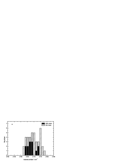
Figure 1: (a) Observed peak-centre positions of the XCN band toward all 39 low- and high-mass YSO’s studied here. Bands originating in high-mass YSO spectra are represented in black, all other YSO’s (dominated by low-mass objects) are hatched. Peak centres are binned at 1.6 cm^-1. (b) Peak-centre positions of laboratory spectra of the $\nu_{3}$ vibrational band of solid OCN^- in a variety of interstellar ice analogues, also summarised in Tables 1 and 2. H₂O- and CH₃OH-rich ices are shown in black, H₂O- and CH₃OH-free ices are hatched, and those thermally annealed to $\geq$ 110 K are white. These centre positions are rounded to the nearest integer wavenumber (cm^-1).

Figure 2: The distribution of centre positions of the XCN band toward the various lines-of-sight in bins of 1.6 cm^-1 including the uncertainties derived from the Monte-Carlo simulations. The Gaussian at 2168.7 cm^-1 is obtained from a single Gaussian fit to the full data set, that at 2166.9 cm^-1 from a similar fit excluding all XCN band centres $\geq$ 2172 cm^-1. This analysis strengthens the conclusion that two components are present in the observational data. The dashed line indicates the maximum wavenumber beyond which no laboratory-based $\nu_{3}$(OCN^-) feature has been found in interstellar ice analogues.

2 Observations

2.1 Observational details

This work uses the $M$-band spectra of a large sample of deeply embedded young stars, which were first presented in Paper I. The data are part of a 3–5 $\mu$m spectroscopic survey of low-mass embedded objects in the nearest star-forming clouds ($\rho$ Oph, Serpens, Orion, Corona Australis, Chamaeleon, Vela, and Taurus) using the Infrared Spectrometer And Array Camera (ISAAC) mounted on UT1-Antu of the Very Large Telescope (VLT) (van Dishoeck et al., 2003). All sources have spectral energy distributions representative of Class I objects, with typical lifetimes of $\sim$ 10⁵ yr since cloud collapse. The $M$-band spectra were obtained in the 4.53–4.90 $\mu$m (2208–2040 cm^-1) range using the medium resolution mode, resulting in a resolving power of $\lambda$/$\Delta\lambda$ = 5000-10000. The reduction of the spectra is described in detail in Paper I. In short, the spectra were corrected for telluric absorption, flux-calibrated relative to bright early-type standard stars, and wavelength-calibrated relative to telluric absorption lines in the standard star spectrum with an accuracy of $\sim$ 5 km s^-1. The final optical depth spectra were derived by fitting a blackbody continuum to the 4.52-4.55 $\mu$m (2212–2198 cm^-1) and 4.76-4.80 $\mu$m (2101–2083 cm^-1) regions, where no features are expected, taking care to exclude known gas-phase lines from the fit. The short wavelength end of the spectra is more noisy due to the onset of the strong telluric CO₂ features.

In addition, spectra of 5 high-mass sources taken from the ISO-SWS data archive, i.e. AFGL 2136, NGC 7538 IRS1, RAFGL 7009S, AFGL 989 and W 33A, were added to the sample.

2.2 The XCN band

In addition to the CO-ice band, a weak secondary feature was detected in a significant subset of the lines of sight. In Paper I this feature was reasonably well reproduced using a single Gaussian whose peak-centre position varied significantly (from 2162 to 2194 cm^-1) and Full Width Half Maxima (FWHM) ranged from 9 to 36 cm^-1. This distribution is summarised in Fig. 1a, where the peak-centres of all XCN bands in the observed sample are plotted, together with the data from the ISO sources.
Careful inspection of the XCN band shows that in some sources like W33 A the feature peaks at 2165.7 cm^-1 whereas in other sources like Elias 32 and IRS 63 the feature is shifted much further to the blue, around 2175 cm^-1. This conclusion that two components underlie the XCN band is supported by a statistical analysis of the observed centre positions shown in Fig. 2. The uncertainties in the observed distribution were quantified using a Monte Carlo approach. Each Monte Carlo run varies the XCN band centre position of each source within a normal distribution with a standard deviation from peak-centre position as found in Paper I. This produces a perturbed distribution allowed within the uncertainties on the band positions. By calculating a large number ($10^{5}$) of perturbed distributions, an uncertainty on the number of sources within each wavenumber bin can be estimated by simply deriving the standard deviation for the set of perturbed distributions. A single Gaussian distribution centred at 2168.7 $\pm$ 1.9 cm^-1 ($\chi^{2}$ = 5.58) is seen to give a poor fit. When all bands centred at $\geq$ 2172 cm^-1 are excluded from the fit, the centre of the Gaussian distribution shifts to 2166.9 $\pm$ 1.5 cm^-1 ($\chi^{2}$ = 1.57). The converging $\chi^{2}$ confirms that two components, i.e. one centred at around 2166 cm^-1 and one at around 2175 cm^-1, provide a much better fit.

2.3 H₂O-ice column densities

In order to derive the OCN^- abundances, water ice column densities were estimated using $L$-band spectra (2.85–4.2 $\mu$m) from the same survey (Dartois et al., in prep.). Optical depth spectra of the H₂O-ice feature were obtained by fitting a blackbody spectrum to a $K$-band photometric point from the 2MASS point source catalogue and the available spectroscopic points in the $L$- and $M$-band spectra at wavelengths longer than 3.8 $\mu$m. Care was taken to exclude any hydrogen recombination lines from the fit. Estimated uncertainties in the water ice optical depths are $\sim$ 20%, mainly due to the variable near-infrared fluxes of embedded young stars (see e.g. Kaas, 1999). The optical depths were converted to column densities using a factor of $1.56\times 10^{18}\,\rm cm^{-2}$. This factor was derived by integrating over a laboratory-based H₂O spectrum fitted to the highest quality water bands and scaling with a band strength of $2\times 10^{-16}\,\rm cm\,molec.^{-1}$ (Gerakines et al., 1995).

Table 1: Laboratory experiments on the spectroscopy of $\nu_{3}$(OCN^-) in interstellar ice analogues (T = 10-100 K) ^a

T	Energetic	Ice composition	$\nu_{3}$(OCN-)	FWHM	ref.
(K)	processing	(spectral resolution where known /cm-1)	(cm-1)	(cm-1)
10	ion (30keV)	H2O/CH4/NH3 = 5:4:2 (2)	2170		1
10	thermal	HNCO/NH3 = 1:10 (0.5)	2151		2
10	UV (at 10K)	H2O/CO/CH4/NH3 = 6:2:1:1 (2)	2167	25	3
10	UV (at 10K)	CO/NH3 = 3:1	2155		4
10	UV (at 10K)	H2O/CO/CH3OH/NH3 = 100:10:50:10	2168		5
10	UV (at 10K)	H2O/CO/CH3OH/CnH2n+2/NH3 = 100:10:50:10:10 (0.9)	2160		6
12	UV (at 12K)	HNCO/NH3 = 1:1 (2)	2155		7
12	UV (at 12K)	HNCO/NH3 = 1:100 (2)	2155		7
12	UV (at 10K)	CO/NH3 = 1:40 (2)	2152		7
12	UV (at 30K)	CO/NH3 = 1:40 (2)	2152		7
12	ion (60keV)	CO2/N2 = 1:1 (1)	2168		8
15	proton (0.8MeV)	H2O/CO/NH3 = 5:1:1 (4)	2167	26	9
15	proton (0.8MeV)	H2O/CO2/NH3 = 1:1:2 (4)	2164	25	9
15	proton (0.8MeV)	H2O/CH4/NH3 = 1:1:1 (4)	2159	23	9
15	proton (0.8MeV)	H2O/CO2/N2 = 5:1:1 (4)	2170	25	9
15	proton (0.8MeV)	H2O/CH4/N2 = 1:1:1 (4)	2159	27	9
15	proton (0.8MeV)	CO/NH3 = 1:1 (4)	2164	27	9
15	proton (0.8MeV)	CO2/NH3 = 1:2 (4)	2158	26	9
15	proton (0.8MeV)	CO/N2 = 1:1 (4)	2164	27	10
15	proton (0.8MeV)	CO/N2 = 1:2 (4)	2158	26	10
15	UV (at 15K)	H2O/HNCO/NH3 = 120:1:10 (2)	2169	25	11
15	UV (at 15K)	H2O/HNCO/NH3 = 120:1:10 (2)	2171	25	11
15	UV (at 15K)	HNCO/NH3 = 1:10 (2)	2160	20	11
15	UV (at 15K)	H2O/HNCO/NH3 = 140:8:1 (2)	2165	25	11
20	proton (1MeV)	H2O/CH4/NH3 = 1:2:3	2170		12
20	proton (1MeV)	H2O/CH4/NH3 = 1:2:4	2170		12
20	proton (1MeV)	H2O/CH4/NH3 = 2:4:7	2170		12
20	proton (1MeV)	H2O/CH4/NH3 = 1:7:10	2170		12
20	proton (1MeV)	H2O/CH4/NH3 = 1:3:6	2170		12
20	proton (1MeV)	H2O/CH4/NH3 = 1:3:3	2170		12
20	proton (1MeV)	H2O/CH4/NH3 = 1:4:3	2170		12
20	proton (1MeV)	H2O/CH4/NH3 = 15:7:9	2170		12
20	proton (1MeV)	H2O/CH4/N2 = 1:1:1	2170		12
20	proton (1MeV)	H2O/CO/N2 = 5:1:1	2170		12
20	proton (1MeV)	H2O/CO/NH3 = 2:2:1	2170		12
20	proton (1MeV)	H2O/CO/NH3 = 2:1:3	2170		12
20	proton (1MeV)	H2O/CO/NH3 = 5:1:10	2170		12
30	UV (at 12K)	HNCO/NH3 = 1:100	2155		7
30	thermal	HNCO/NH3/Ar = 2:2:1000 (0.125)	2157		2
30	UV (at 10K)	H2O/CO/CH3OH/CnH2n+2/NH3 = 100:10:50:10:10 (0.9)	2163		6
35	proton (0.8 MeV)	CO/CH4/N2 = 1:1:100 (1)	2166	25	13
50	UV (at 12K)	HNCO/NH3 = 1:100 (2)	2154		7
50	UV (at 37K)	CO/NH3 = 1:1 (2)	2158		7
55	UV (at 10K)	H2O/CO/CH3OH/CnH2n+2/NH3 = 100:10:50:10:10 (0.9)	2163		6
60	UV (at 12K)	HNCO/NH3 = 1:100 (2)	2154		7
80	UV (at 12K)	CO/NH3 = 1:1 (4)	2157		14
80	UV (at 12K)	H2O/CO/NH3 = 1:1:1 (4)	2160		14
80	UV (at 12K)	H2O/CO/NH3 = 2:1:1 (4)	2163		14
80	UV (at 12K)	H2O/CO/NH3 = 3:1:1 (4)	2166		14
100	UV (at 37K)	CO/NH3 = 1:1	2163		15
100	UV (at 37K)	CO/NH3 = 1:1 (2)	2157		7
100	ion (60keV)	CO2/N2 = 1:1 (1)	2165		8
100	UV (at 10K)	H2O/CO/CH3OH/NH3 = 100:10:50:10	2166		5
100	UV (at 10K)	H2O/CO/CH3OH/CnH2n+2/NH3 = 100:10:50:10:10 (0.9)	2163		6

• ^aExperiments in italics show ices that lack H₂O. All $\nu_{3}$ peak-positions are rounded up or down to the nearest integer wavenumber. ¹ Strazzulla & Palumbo (1998), ² Raunier et al. (2003), ³ d’Hendecourt et al. (1986), ⁴ Lacy et al. (1984), ⁵ Tegler et al. (1993), ⁶ Allamandola et al. (1988), ⁷ Novozamsky et al. (2001), ⁸ Palumbo et al. (2000), ⁹ Hudson & Moore (2000), ¹⁰ Hudson et al. (2001), ¹¹ van Broekhuizen et al. (2004), ¹² Moore et al. (1983), ¹³ Moore & Hudson (2003), ¹⁴ Grim & Greenberg (1987), ¹⁵ Bernstein et al. (2000)

Table 2: Laboratory experiments on the spectroscopy of OCN^- in interstellar ice analogues (T $>$ 100K) ^a

T	Energetic	Ice composition	$\nu_{3}$(OCN-)	FWHM	ref.
(K)	processing	(spectral resolution where known /cm-1)	(cm-1)	(cm-1)
110	thermal	H2O/HNCO/Ar = 12:1:1000 (0.12)	2170		1
120	UV (at 10K)	CO/NH3 = 1:1	2155		2
120	UV (at 15K)	H2O/HNCO/NH3 = 120:1:10 (2)	2166	22	3
130	thermal	H2O/HNCO = 10:1 (0.5)	2172		1
140	UV (at 37K)	CO/NH3 = 1:1 (2)	2159		4
150	ion (60keV)	CO2/N2 = 1:1 (1)	2163		5
150	UV (at 10K)	CO/NH3 = 3:1	2165		6
150	UV (at 10K)	H2O/CO/CH3OH/NH3 = 100:10:50:10	2162		7
160	thermal	HNCO/NH3 = 1:10 (0.5)	2165		1
180	UV (at 12K)	CO/NH3 = 1:1 (4)	2157		8
180	UV (at 12K)	CO/NH3 = 1:10 (4)	2157		8
200	ion (60keV)	CO2/N2 = 1:1 (1)	2162		5
200	UV (at 10K)	H2O/CO/CH4/NH3 = 6:2:1:1 (2)	2167	25	9
200	UV (at 10K)	H2O/CO/CH3OH/NH3 = 100:10:50:10	2164		7
200	UV (at 10K)	H2O/CO/CH3OH/NH3 = 100:10:50:10 (0.9)	2165		10
200	UV (at 10K)	H2O/CO/CH3OH/CnH2n+2/NH3 = 100:10:50:10:10 (0.9)	2164		10
200	UV (at 10K)	H2O/CO/CH3OH/CnH2n+2/NH3 = 100:10:50:10:10 (0.9)	2163		10

• ^aExperiments in italics show ices that lack H₂O. All $\nu_{3}$ peak-positions are rounded up or down to the nearest integer wavenumber. ¹ Raunier et al. (2003), ² Schutte & Greenberg (1997), ³ van Broekhuizen et al. (2004), ⁴ Novozamsky et al. (2001), ⁵ Palumbo et al. (2000), ⁶ Lacy et al. (1984), ⁷ Tegler et al. (1993), ⁸ Grim & Greenberg (1987) ⁹ d’Hendecourt et al. (1986), ¹⁰ Allamandola et al. (1988)

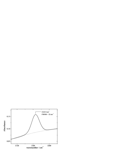
Figure 3: Example of a laboratory spectrum of $\nu_{3}$(OCN^-), obtained after thermal annealing to 120 K of an ice composed of H₂O/HNCO/NH₃ = 120/1/10 (grey curve). After accounting for the baseline (dotted line), an excellent fit to the laboratory data is obtained with a single Gaussian fit, centred at 2165.9 cm^-1, FWHM = 23 cm^-1 (black curve).

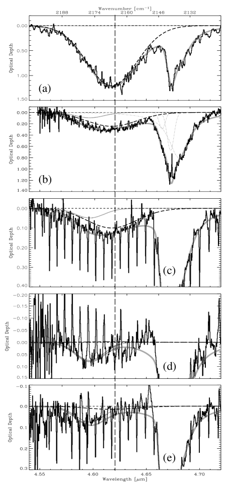
Figure 4: The XCN band as observed in the line-of-sight toward five YSO’s, ordered from top to bottom from the most red-centred to the most blue-centred band, i.e. (a) W33 A, (b) HH 46, (c) Reipurth 50, (d) Elias 32 and (e) IRS 63. All spectra (black) are continuum subtracted (small-dashed line) and the total fit is shown (grey curve). The two components underlying the XCN band, i.e. the 2165.7-component (dashed curve) and the 2175.4-component (dotted curve) are shown. The three-component fit to the solid CO band at 4.67 $\mu$m (2139 cm^-1) is shown only in (b) by the three grey dash-dotted curves. The vertical dashed line at 4.62 $\mu$m guides the eye.

3 Laboratory experiments on OCN^- pertinent to the XCN band analysis

3.1 Spectroscopy

The formation and infrared spectroscopy of solid OCN^- has been studied extensively in numerous laboratories. Its spectrum is dominated by the CN stretching-vibration (the $\nu_{3}$ band), which can be well fitted by a single Gaussian profile (see for example Fig. 3). In Tables 1 and 2 an overview is given of all (to the best of our knowledge) published peak centres and FWHM of the $\nu_{3}$ band of OCN^-, as measured in the laboratory under conditions relevant to the interstellar case, e.g. matrix-isolation studies have been excluded. In addition, information is tabulated on the initial ice composition, ice temperature and processing mechanism applied to the ice. With the exception of H₂O, CH₃OH and NH₃, most of the other ice components have fully desorbed by 120 K under high-vacuum laboratory conditions but OCN^- remains in the solid state, stabilised by a counter ion (possibly NH${}_{4}^{+}$, Demyk et al., 1998; Taban et al., 2003). Hence, Table 1 contains those experiments in which the ice matrix is predominantly intact, whereas Table 2 summarises those in which most ice constituents have desorbed or are desorbing.
Fig. 1b shows the distribution of peak centres of the laboratory $\nu_{3}$ of the OCN^- feature highlighting the initial ice environment, i.e. H₂O- or CH₃OH-rich (black), H₂O- and CH₃OH-lacking (hatched) and thermally annealed, i.e. those listed in Table 2 ($T$ $\geq$ 110 K, white). It is important to note that this histogram is significantly weighted by the parameter space investigated in the laboratory. Peak centres vary strongly with ice composition, ranging from 2151 to 2172 cm^-1. Within this range, $\nu_{3}$(OCN^-) peaks at between 2151–2160 cm^-1 in the absence of H₂O and CH₃OH (Novozamsky et al., 2001; Raunier et al., 2003; Grim & Greenberg, 1987; Hudson & Moore, 2000), or at between 2160–2172 cm^-1 when associated with a strongly hydrogen-bonding environment, i.e. H₂O- or CH₃OH-rich ices (Grim & Greenberg, 1987). No trend is apparent in the data relating the actual formation mechanism of OCN^- to its band position.
From Fig. 1b is also clear that in warm ices ($T\geq$ 110 K), $\nu_{3}$(OCN^-) peaks at similar positions to the colder ices. However within a single ice matrix, thermal annealing beyond 100 K tends to shift the $\nu_{3}$(OCN^-) peak to between 2155 and 2167 cm^-1 when OCN^- is stabilised by NH${}_{4}^{+}$ (Novozamsky et al., 2001; Palumbo et al., 2000). In the exclusive presence of H₂O (i.e. for H₂O/HNCO and H₂O/HNCO/Ar), however, $\nu_{3}$(OCN^-) must be stabilised by water solvation (most plausibly H₃O⁺) and seems thermally unaffected, peaking at 2170 to 2172 cm^-1.
The spectral range of peak positions observed for laboratory $\nu_{3}$(OCN^-) implies that only one component of the observed XCN-bands can be associated with OCN^-. No laboratory $\nu_{3}$(OCN^-) spectrum in Fig. 1b peaks beyond 2172 cm^-1, whereas a significant fraction of the astronomical spectra in Fig. 1a peaks around 2175 cm^-1. This is emphasised by the dashed line in Fig. 2, indicating that only those XCN-bands represented by the Gaussian fit to the left of the dashed line can be matched to a laboratory spectrum of OCN^-. The peak centres of these XCN-bands can be explained by OCN^- residing in a strong hydrogen-bonding ice environment that may have been thermally annealed up to 200 K. OCN^- embedded in an ice that lacks a strong hydrogen-bonding network generally peaks red-wards of the XCN-bands observed, even after thermal annealing, causing this kind of ice to be an unlikely interstellar OCN^- environment.

3.2 Band strength

The reported value of the $\nu_{3}$(OCN^-) band strength, $A_{\rm OCN^{-}}$, varies considerably in the literature. Lacy et al. (1984) assumed $A_{\rm OCN^{-}}$ $\leq$ 1.0$\times$10^-17 cm molec.^-1, based on the assumption that the cross section of a typical CN-stretching vibration is approximately 5 times less than that of a CO-stretch. d’Hendecourt et al. (1986) derived $A_{\rm OCN^{-}}$ from photolysis experiments to be 1.8–3.6$\times$10^-17 cm molec.^-1, assuming a constant carbon budget per experiment, followed by Demyk et al. (1998), who assumed a constant oxygen budget to obtain $A_{\rm OCN^{-}}$ $\geq$ 4.3$\times$10^-17 cm molec.^-1. Both studies probably underestimated the value of $A_{\rm OCN^{-}}$ due to the formation of infrared-weak or inactive photoproducts, and the neglect of photodesorption of volatile species like CO and CO₂ (van Broekhuizen et al. in prep).
More recently, van Broekhuizen et al. (2004) determined $A_{\rm OCN^{-}}$ from the thermal deprotonation of HNCO by NH₃, using the NH₃ to NH${}_{4}^{+}$ conversion as reference, giving $A_{\rm OCN^{-}}$ = 1.3$\times$10^-16 cm molec.^-1. In the present analysis of the XCN band, this value of $A_{\rm OCN^{-}}$ has been adopted because its determination is not influenced by any photodesorption or the formation of photo-products (both known and unknown), which may have affected the previously derived values. The adopted band strength does not affect any subsequent conclusions in this paper on the photo-production of OCN^-, since these reaction efficiencies were derived using the same value of the band strength. However, the adopted $A_{\rm OCN^{-}}$ value does impact on the conclusions drawn if OCN^- is thermally formed, because significantly more HNCO will be required in the solid state if a smaller value of $A_{\rm OCN^{-}}$ were used.

3.3 Formation mechanisms

The presence of OCN^- in interstellar ices has become widely cited as a probe of energetic processing of the protostellar environment, in particular by ultraviolet (UV) photons. However, this assumption has been challenged on the basis of a quantitative set of laboratory experiments studying the efficiency of OCN^- photoproduction, and the possibilities of forming OCN^- thermally (Raunier et al., 2003; van Broekhuizen et al., 2004). To assist the reader in following the subsequent discussions and conclusions of this paper, these two OCN^- formation mechanisms, and the regimes in which they apply, are summarised below.
In the laboratory, photochemical processes lead to the formation of OCN^- at abundances of (at most) 1.9 % with respect to H₂O-ice, starting from an interstellar ice analogue containing H₂O, CO and NH₃ (van Broekhuizen et al., 2004). The initial amount of NH₃ in these experiments ranges from 8 to 40% with respect to H₂O ice. The abundance of interstellar NH₃ is uncertain, but is observed to be $<$5% toward W33 A (Taban et al., 2003). Including the constraint that the abundance of NH₃ ice after photolysis cannot be more than 5% lowers the maximum OCN^- photoproduction yield to 1.2 % with respect to H₂O ice (see, for example, Figure 6 of van Broekhuizen et al., 2004).
From these experiments, the maximum interstellar OCN^- photoproduction yield was constrained to an abundance of 1.2 % with respect to H₂O-ice by assuming a maximum abundance for solid NH₃ of 5 % with respect to H₂O-ice, as observed toward W 33A (Taban et al., 2003). If the cosmic ray induced UV-field (1.4$\times$10³ photons cm^-2 s^-1, Prasad & Tarafdar, 1983) is assumed to be the only source of UV-photons, this maximum 1.2 % OCN^- abundance would be reached after a UV-fluence equivalent to a molecular cloud lifetime of 4$\times$10⁸ years. This is long compared to the assumed age of the YSO’s studied in this paper ($\sim$10⁵ yr), even if a long pre-stellar phase of $\sim$ 10⁷  yr is included.
Alternatively, laboratory studies show that OCN^- can be formed via thermal heating of ices containing HNCO in the presence of NH₃ or H₂O with an efficiency of 15-100 % (Demyk et al., 1998; Raunier et al., 2003; van Broekhuizen et al., 2004). Laboratory experiments and theoretical calculations show that this solvation process is even efficient at 15 K provided that HNCO is sufficiently diluted in NH₃ or H₂O-ice (Raunier et al., 2003; Park & Woon, 2004), for the proton transfer to occur.

Table 3: Components adopted in the fit of the observed XCN bands

	2165.7-component	2175.4-component
Line profile	Gaussian	Gaussian
Centre (cm-1)	2165.7	2175.4
FWHM (cm-1)	26	15

4 Decomposition of the XCN profile

Our analysis of the XCN band, containing two components (see Sect. 2.2), refines the results from Paper I where a single component fit was used. The component centred at $\sim$ 2175 cm^-1 has been discussed in detail by Fraser et al. (2005) in terms of gas-surface interactions of CO with interstellar grains. Thus, in the remainder of this paper the discussion is focused on the carrier of the component of the XCN band centred at $\sim$2166 cm^-1, and simply uses a two component fit to correct for any contribution from the component centred at $\sim$ 2175 cm^-1.
The distribution of the $\sim$2166 cm^-1 component of the XCN band shows a broad spread of band centres, most probably related to source-to-source differences in the local ice-environment of the carrier of this component in the various lines-of-sight. A good ‘prototype’ for this component is the XCN band of W33 A, as it is also one of the most red-centred and strongest of the objects studied. It matches a Gaussian profile, peaking at 2165.7 $\pm$ 0.1 cm^-1 (FWHM = 26 $\pm$ 1 cm^-1), that is well reproduced by laboratory spectra of OCN^- (see Fig. 3). An initial analysis showed that this Gaussian profile also reproduces the red wing and component of the XCN band of all other YSO’s in this study. Consequently, the XCN band was analysed using a similar procedure to that employed for the 6.8 $\mu$m band by Keane et al. (2001), whereby the 6.8 $\mu$m band was also decomposed by using the most extreme source in the sample, Mon R2:IRS3, to fit all lines-of-sight together with a ‘rest-spectrum’ obtained after the initial fitting of the other sources. Here, the Gaussian fit to the W33 A XCN band is adopted (henceforth referred to as the 2165.7-component), and not the actual YSO spectrum, to avoid any contribution from the CO-ice band to the fit.
The component underlying the distribution of XCN bands centred at $\sim$2175 cm^-1 in Fig. 2 was determined empirically, in effect by fitting the residual of the XCN band after spectral subtraction of the contribution of the 2165.7-component. This resulted in a Gaussian, centred at 2175.4 $\pm$ 3 cm^-1 (FWHM = 15 $\pm$ 6 cm^-1). This feature will be referred to as the 2175.4-component. Adopting a different Gaussian for the 2165.7-component, i.e. one centred at 2166.9 or 2168.7 cm^-1, does not significantly affect these fit results, which indicates that the range of environments observed for the 2165.7-component do not introduce an error on the fit.
The fitting routine is based on the same IDL algorithms developed in Paper I. All spectra were fitted using the same 2165.7- and 2175.4-components, keeping the centre positions and FWHM constant. The optical depths of the two components are the only free parameters (see Table 3 for a summary). In addition, a full fit of the CO-ice feature was run in parallel to correct for possible overlap between the wing of the CO-ice feature and the XCN band (see Paper I and Fig. 4b for details on the CO-ice fit).

5 Results

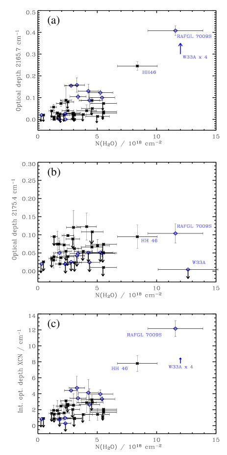
Figure 5: (a) The optical depth of the 2165.7-component, (b) the optical depth of the 2175.4-component, and (c) the total integrated area of the XCN band, as determined by Eq.1, are shown versus the H₂O ice column density, $N$(H₂O). High-mass objects are indicated by diamonds, all others, dominated by low-mass YSO’s, by stars. 3 $\sigma$ uncertainties are given, or upper limits are indicated by arrows.

5.1 Results of the fitting procedure

Fig. 4 shows the results of fitting the XCN band in five of the YSO’s in our sample. These are presented from top to bottom in order of decreasing wavelength of the XCN band centre position. The XCN band of W33 A (Fig. 4a) shows the excellent fit of the 2165.7-component with $\leq$ 1 % contribution by the 2175.4-component. In Fig. 4b, already some contribution to this band from the 2175.4-component is apparent. From Fig. 4b to e, the 2175.4-component contribution increases, blue-shifting the XCN band, until it dominates the XCN band toward Elias 32 and IRS 63. Table 4 summarises the derived optical depths. The $\chi^{2}$ of the fit (not shown) generally varies between 0.3 and 10. The additional three-component fit of the solid CO feature (Paper I) is shown by the three grey dash-dotted curves in Fig. 4b only, but was applied to all fits.

5.2 Correlations with H₂O

In Fig. 5a, the optical depth of the 2165.7-component is plotted against the H₂O column density, $N$(H₂O). For all YSO’s studied here, the derived optical depth of the 2165.7-component is $\leq$ 0.16, except for HH 46, RAFGL 7009S and W33 A. No relationship with $N$(H₂O) is apparent. In fact, it seems that the optical depth value of the 2165.7-component toward high-mass YSO’s is in most cases larger than toward lower mass YSO’s, where the optical depth is typically $\leq$ 0.09.
Fig. 5b presents the optical depth of the 2175.4-component plotted against $N$(H₂O). The optical depth of the 2175.4-component is $\leq$0.14 for all sources in this study and is not correlated to the H₂O column density. An interpretation of this feature is given by Fraser et al. (2005).
Comparing Figs. 5a and 5b shows that the 2165.7-component dominates the XCN band toward most high-mass YSO’s, whereas the 2175.4-component contributes most to the XCN band in all other sources. Checks of a possible relationship between the optical depth of the two components (not shown) proved negative, indicating that the components do not trace the same feature.
In Fig. 5c the total integrated area of the XCN band is plotted against $N$(H₂O). The total integrated area of the XCN band is derived from the sum of the integrated areas of the individual components

$${\int{\tau_{\rm(XCN)}\,d\nu}}={\int{\tau_{2165.7}\,d\nu}}+{\int{\tau_{2175.4}\,d\nu}}$$ (1)

The XCN band is evenly distributed toward high- and low-mass YSO’s and its total area tentatively increases with increasing $N$(H₂O).

5.3 Correlations with CO

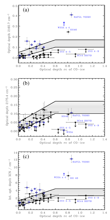
Figure 6: (a) The optical depth of the 2165.7-component, (b) the optical depth of the 2175.4-component, and (c) the total integrated area of the XCN band, as determined by Eq.1, are presented versus the optical depth of the red component (rc) of CO-ice. High-mass objects are indicated by diamonds, all others, dominated by low-mass YSO’s, by stars. 3 $\sigma$ uncertainties are given, or upper limits are indicated by arrows. The shaded area, shown in each plot, marks the correlation between the optical depth of the XCN band and the red component (rc) of CO-ice as proposed by Paper I.

The CO-ice band, observed at around 2140 cm^-1 toward all lines-of-sight here, has been analysed in detail in Paper I, using a phenomenological decomposition into 3 components to fit its band profile. The most red-centred component (rc) was attributed to CO in a hydrogen-bonded environment, although this cannot fully explain its extended red wing. It was suggested that the rc may evolve from pure CO-ice when thermal annealing of the ice induces CO to migrate into, and get trapped in, porous H₂O-ice. As such, this component may trace the thermal history of the interstellar ice mantle (Tielens et al., 1991, Paper I). Hence, the relationship between the optical depth of the rc of CO-ice and the XCN band may provide information on the thermal history of the XCN band as well. Paper I found a tentative correlation between this rc and the optical depth of the XCN band and suggested that this was actually due to a component of the XCN band, centred between 2170-2180 cm^-1.
Fig. 6a presents the optical depth of the 2165.7-component versus the optical depth of the rc of the CO-ice band, showing that this component and the rc of CO-ice are not correlated. The shaded area marks the correlation suggested by Paper I. However, those sources that show a strong 2165.7-component also tend to have a strong CO rc, but not the other way around.
In Fig. 6b the optical depth of the 2175.4-component is plotted against the optical depth of the rc of the CO-ice band. In contrast to the 2165.7-component, the 2175.4-component matches the correlation indicated by the shaded area much better, particularly at rc optical depths of below 0.6, corroborating the idea posed by Paper I. However, the YSO’s with deep rc optical depths (and deep 2165.7-component optical depths) fall outside the correlation proposed by Paper I.
For completion, Fig. 6c illustrates the relation between the integrated area of the XCN band and the optical depth of the rc of CO-ice, showing that most low-mass YSO’s match the correlation suggested by Paper I (shaded area) and reflecting that in these objects the 2175.4-component dominates the XCN band (see Sect. 5.2). Conversely, approximately half of the XCN bands observed toward high-mass YSO’s clearly exhibit larger integrated areas than would be expected from that correlation.

6 Discussion

6.1 The OCN^- abundance

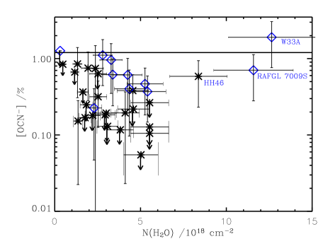
Figure 7: The OCN^- abundance, [OCN^-], plotted with respect to the H₂O column density, $N$(H₂O). High-mass objects are indicated by diamonds, all others, dominated by low-mass YSO’s, by stars. 3 $\sigma$ uncertainties are given, or upper limits are indicated by arrows. The black horizontal line marks the 1.2 % maximum abundance of OCN^- that may be formed photochemically under interstellar conditions, as determined from laboratory studies.

Based on the discussion in Sect. 3.1, only the 2165.7-component of the astronomical spectra can be confidently assigned to OCN^-. Thus, the OCN^- column density, $N$(OCN^-), and its abundance with respect to H₂O, [OCN^-], are derived from the optical depth of the 2165.7-component via:

$${\rm[OCN^{-}]}={\frac{N({\rm OCN^{-}})}{N({\rm H_{2}O})}}={\frac{{\int{\tau_{\rm 2165.7}\,d\nu}\times{A_{\rm OCN^{-}}^{-1}}}}{N({\rm H_{2}O})}}$$ (2)

where the FWHM of $\tau_{\rm 2165.7}$ is fixed at 26 cm^-1 and $A_{\rm OCN^{-}}$ is 1.3$\times$10^-16 cm molec.^-1 (van Broekhuizen et al., 2004, see Sect. 3.2 for a discussion on the value of $A_{\rm OCN^{-}}$). The inferred $N$(OCN^-) and [OCN^-] are summarised in Table 4.

In Fig. 7 the OCN^- abundance with respect to $N$(H₂O), [OCN^-], is plotted against $N$(H₂O). All sources studied here show abundances of $\leq$1.0 %, except for W33 A. Excluding the high-mass stars, gives abundances of $\leq$ 0.85 %. The high signal-to-noise of the spectra allows the detection of the XCN band down to optical depths of 0.01. As a result, very strict upper limits have been put on the OCN^- abundance along some lines of sight.

Table 4: Results of the XCN band fitting procedure

Source a	$\tau$(2165.7)b	$\tau$(2175.4)b	$N$(OCN-)c	[OCN-]c	$\tau$(H2O) d
	2165.7 cm-1	2175.4 cm-1	$\times$1016 molec. cm-2	%
$\rho$ Ophiuchus
IRS42	$\leq$0.023	0.020$\pm$0.010	$\leq$0.46	$\leq$0.25	1.17
IRS43	$\leq$0.02	0.072$\pm$0.030	$\leq$0.40	$\leq$0.18	1.40
IRS44	$\leq$0.02	$\leq$0.024	$\leq$0.40	$\leq$0.13	1.95
IRS46	$\leq$0.039	$\leq$0.035	$\leq$0.78	$\leq$0.68	0.74
IRS51	0.073$\pm$0.013	0.037$\pm$0.015	1.46$\pm$0.26	0.76$\pm$0.12	1.23
IRS63	$\leq$0.015	0.075$\pm$0.016	$\leq$0.3	$\leq$0.17	1.12
WL12	-	0.062$\pm$0.032	-	-	1.95
CRBR 2422.8	$\leq$0.029	0.120$\pm$0.045	$\leq$0.58	$\leq$0.19	1.90
Elias 32	$\leq$0.030	0.074$\pm$0.036	$\leq$0.60	$\leq$0.36	1.04
VSSG17	-	$\leq$0.095	-	-	0.87
RNO 91	0.087$\pm$0.010	0.066$\pm$0.017	1.74$\pm$0.2	0.40$\pm$0.09	2.88
Serpens
EC90 A	0.010$\pm$0.006	0.039$\pm$0.008	0.2$\pm$0.12	0.15$\pm$0.05	0.86
EC90 B	0.056$\pm$0.012	0.030$\pm$0.007	1.12$\pm$0.24	0.86$\pm$0.12	0.84
EC82	$\leq$0.02	$\leq$0.026	$\leq$0.40	$\leq$0.86	0.30
CK2	$\leq$0.027	$\leq$0.089	$\leq$0.54	$\leq$0.19	1.86$\pm$0.19 e
SVS 4-9	$\leq$0.08	$\leq$0.04	$\leq$1.60	$\leq$0.64	1.6$\pm$0.1 f
SVS 4-5	$\leq$0.073	$\leq$0.010	$\leq$1.46	$\leq$0.27	3.50$\pm$0.30 f
Orion
TPSC 78	0.155$\pm$0.003	$\leq$0.025	3.1$\pm$0.06	1.12$\pm$0.14	1.77
TPSC 1	0.158$\pm$0.032	$\leq$0.042	3.16$\pm$0.64	0.97$\pm$0.13	2.08
Reipurth 50	0.100$\pm$0.005	0.049$\pm$0.012	2.0$\pm$0.1	0.38$\pm$0.08	3.42
Corona Australis
HH100 IRS	0.04$\pm$0.002	0.098$\pm$0.003	0.8$\pm$0.04	0.32$\pm$0.08	1.6
HH46	0.245$\pm$0.019	0.095$\pm$0.032	4.9$\pm$0.38	0.59$\pm$0.01	5.3$\pm$3.0 g
RCrA IRS7A	$\leq$0.029	$\leq$0.074	$\leq$0.58	$\leq$0.11	3.5
RCrA IRS7B	$\leq$0.035	$\leq$0.050	$\leq$0.70	$\leq$0.13	3.5
RCrA IRS5A	0.040$\pm$0.025	0.123$\pm$0.036	0.80$\pm$0.5	0.20$\pm$0.06	2.60
RCrA IRS5B	$\leq$0.022	$\leq$0.054	$\leq$0.44	$\leq$0.12	2.42
Chamaeleon
ChaIRN	0.088$\pm$0.069	$\leq$0.055	1.76$\pm$1.38	0.75$\pm$0.12	1.5
ChaIRS 6A	$\leq$0.05	$\leq$0.108	$\leq$1.0	$\leq$0.22	2.90
Vela
LLN17	0.104$\pm$0.011	0.048$\pm$0.014	2.08$\pm$0.22	0.62$\pm$0.11	2.14
LLN20	0.087$\pm$0.040	$\leq$0.024	1.74$\pm$0.8	0.41$\pm$0.09	2.75
LLN33	0.130$\pm$0.032	$\leq$0.051	2.6$\pm$0.64	0.62$\pm$0.11	2.69
LLN39	$\leq$0.02	$\leq$0.02	$\leq$0.40	$\leq$1.3	0.20
LLN47	-	0.050$\pm$0.033	-	-	1.15
Taurus
LDN 1489 IRS	$\leq$0.014	0.070$\pm$0.016	$\leq$0.28	$\leq$0.06	3.18
Additional sources h
RAFGL 2136	0.123$\pm$0.011	$\leq$0.051	2.46$\pm$0.22	0.47$\pm$0.09	3.33 i
NGC7538 IRS1	-	$\leq$0.019	-	-	1.47
RAFGL 7009S	0.408$\pm$0.021	0.104$\pm$0.026	8.16$\pm$0.42	0.71$\pm$0.11	7.33 j
W33A	1.204$\pm$0.030	$\leq$0.004	24.08$\pm$0.60	1.93$\pm$0.01	8.00$\pm$0.75 k
RAFGL 989	0.026$\pm$0.013	0.019$\pm$0.017	0.52$\pm$0.26	0.23$\pm$0.06	1.45

• ^a Source spectra taken from Paper I, unless otherwise stated. ^b 3$\sigma$ uncertainties or upper limits are given. ^c Column densities and abundances derived from the 2165.7-component using Eq.2. ^d H₂O optical depths from Dartois et al. private communication, unless otherwise stated, and derived according to Sect. 2.1. Uncertainties are between 10 to 20 %. ^e Eiroa & Hodapp (1989) ^f Pontoppidan et al. (2004) ^g Boogert et al. (2004) ^h ISO-data archive. ⁱ Gerakines et al. (1999) ^j Dartois et al. (1999) ^k Gibb et al. (2000)

6.2 OCN^- abundance variations

The sample of XCN observations presented here is large enough to obtain statistically significant information on the distribution of abundances and to compare between different classes of cloud environments, such as low- and high-mass star-forming regions. As seen in Fig. 7 and Table 4, the abundance of OCN^- is observed to vary by at least a factor of 10-20 among the lines of sight in the sample. This observed range of OCN^- abundances is larger than that of CH₃OH and second only to that of ice species whose abundances are sensitive to low-temperature freeze-out and evaporation, such as CO.
A particularly interesting point is that some of the observed lines of sight toward low-mass sources are located in close proximity to each other in the plane of the sky (100-10 000 AU). Such objects provide a direct probe of the physical size of regions with enhanced (or reduced) OCN^- abundances. In particular, several close binaries in the sample probe variations in abundances on scales of a few hundred AU, i.e. at the scale of circumstellar disks. Some of the best upper limits on the OCN^- abundance of $<0.1\,\%$ are observed toward IRS 43 and IRS 44 in the $\rho$ Ophiuchus star-forming cloud. These lines of sight are located approximately $4\arcmin$ or 30 000 AU from IRS 51, which has a measured OCN^- abundance of 0.8 %. This shows that OCN^- is formed in localised regions even within the same low-mass star-forming cloud complex. The individual components of the close binary source EC 90A+B, which were observed separately, appear to have OCN^- abundances varying by a factor of 6. Since the separation between the two components is only 1$\aas@@fstack{\prime\prime}$6, corresponding to approximately 400 AU, this is an indication that processes occurring on the size scale of circumstellar disks may be required to form OCN^- in large quantities. Note, however, the spectrum observed toward EC 90B is complicated by complex emission and absorption from gaseous CO, so that the observed difference in OCN^- abundances for this binary requires further investigation. The two components in another close binary, RCrA IRS5, also show a tentative difference in OCN^- abundance of a factor of 2. Clearly, only slightly more sensitive observations of embedded close binaries will be able to confirm the observation of a varying OCN^- abundance on scales of a few hundred AU.

6.3 OCN^- formation toward low-mass YSOs

The observed abundances and their variations for our large sample of sources put important constraints on the formation mechanism of OCN^-. All inferred OCN^- abundances presented here allow quantitatively for a photochemical formation mechanism (see Sect. 3.3). Only W33 A, an embedded O-type star with a luminosity of $10^{5}\,L_{\odot}$ (Mueller et al., 2002) with an OCN^- abundance of $\sim$ 2% is at the edge of the range, as are the Galactic center source GC:IRS19 and the external galaxy NGC 4945 presented elsewhere (see van Broekhuizen et al. 2004). If we define high- and intermediate mass YSO’s as those more luminous than 50 $L_{\odot}$, it is found that OCN^- abundances of order 0.85–1 % are observed toward high- intermediate- and low-mass stars in our sample, but strict upper limit abundances of $<0.2\,\%$ are observed only toward low-mass stars. This does indicate that some differences exist in the efficiency of OCN^- production between high- and low-mass star-forming regions, and may suggest that UV photons play a role. However, comparison with laboratory studies shows that the photon dose required to produce the highest OCN^- abundances (of $\sim$ 0.85 %) detected here toward low-mass YSO’s are $\sim$ 40 $\times$ larger than can be accounted for by the cosmic ray induced photons that any ice might receive within the typical lifetime of the pre- and protostellar phases (see Sect. 3.3). Adopting the somewhat higher cosmic-ray induced photon fluxes estimated by Shen et al. (2004) would lower these timescales by an order of magnitude, and they could be further decreased by a factor of 2 if the initial NH₃ abundance were as high as 30 %, but it remains difficult to fully reconcile the ages.
Another, perhaps more serious problem with the UV photoproduction scenario is that little variation in the OCN^- abundance from source to source is expected if the cosmic-ray induced photon flux is assumed to be the same everywhere. Thus, local sources of radiation —either UV from the young star or star-disk boundary— need to be invoked to explain the observed small-scale variations. A well-known concern is whether any of this UV radiation is able to reach the bulk of the ices because of the large extinctions involved. Spherically-symmetric models of YSO envelopes have been constructed, taking the variation of the density, dust temperature and UV radiation with depth into account (e.g. Jørgensen et al., 2002), and it has been shown that any UV from the star only reaches the inner few % of the envelope mass (e.g., Stäuber et al., 2004). Thus, special geometries are required to allow the UV to escape and reach the bulk of the ice, such as outflow cavities or flaring turbulent disks in which the ices are cycled from the shielded midplane to the upper layers. One alternative option is UV radiation created by secondary electrons resulting from X-rays from the young star. Model calculations show that the X-rays, and thus the UV radiation, penetrate much deeper into the envelope than the UV from the star itself so that it can reach a larger fraction of the ices (Stäuber et al., 2005). It would be worthwhile to couple such models with an ice chemistry to check the OCN^- production quantitatively, but this is beyond the scope of this paper.
An alternative scenario for OCN^- formation is through thermal heating of HNCO in the presence of NH₃- or H₂O-ices. Assuming a 15–100 % efficiency of this mechanism as determined under laboratory conditions (see Sect. 3.3), the OCN^- abundances toward low-mass YSO’s presented here imply that 0.85–5 % HNCO should be present in the solid state prior to the formation of OCN^- to explain the highest observed abundances of $\sim$0.85 %. To date, HNCO has been detected in interstellar gas associated with star-forming regions, with column densities in the range from 0.3–7.5$\times$10¹⁴ cm^-2 (Wang et al., 2004; Zinchenko et al., 2000; Kuan & Snyder, 1996; Jackson et al., 1984; van Dishoeck et al., 1995). This is a factor of 100 less than what is expected from the OCN^- column densities derived here, assuming all the OCN^- evaporates as HNCO. In the solid state, only HNCO upper limits, of the order of 0.5 to 0.7 % with respect to H₂O-ice, are determined toward W 33A, NGC 7538 IRS9 and AFGL2136 (van Broekhuizen et al., 2004). Toward the low-mass YSO Elias 29, this is $\leq$ 0.3 % (derived from Boogert et al., 2002). The ease with which HNCO is deprotonated in a H₂O-rich environment implies that HNCO would be difficult to detect toward regions where the ice is warmer than 15 K, although its presence may be observable by means of its 4.42 $\mu$m feature toward the coldest regions where the ice temperature is close to 10 K. On the basis of $\tau_{\rm OCN^{-}}$ derived here, and the band strength of HNCO (van Broekhuizen et al., 2004), $\tau_{\rm HNCO}$ is expected to range from 0.001 to 0.08, a factor of 5 less than observed for OCN^-.
Chemical models predict that HNCO is formed on interstellar grains via grain-surface reactions with an abundance upper limit of $\leq$ 1–3 % with respect to H₂O-ice (Hasegawa & Herbst, 1993; Keane et al., 2001). Given the observed upper limits and model abundances for HNCO, thermal processing also has difficulties to explain the highest observed OCN^- abundances, but it is a serious alternative to UV-photoprocessing for the formation of at least a fraction of OCN^- in interstellar ices. The observed OCN^- abundance variations would in this scenario have to result from variations in the grain-surface chemistry rates forming the reactants that lead to OCN^-, for example due to temperature or availability of atomic N.
On the basis of its spectroscopy, it is not possible to draw a distinction between OCN^- formation via proton-, electron-, UV- or thermally induced processes, neither from laboratory spectra (Sect. 3.1), nor from astronomical observations of the $\rm 2165.7\,cm^{-1}$ OCN^- band.

7 Conclusion

The XCN band has been observed toward 39 YSO’s enabling the first detailed study of the OCN^- abundance in a large sample of low-mass YSO’s. Statistical analysis of the band centre position distribution proves unequivocally that the band contains at least two components, of which only one (centred at 2165.7 cm^-1) can be associated with OCN^- as its carrier, based on laboratory OCN^- spectra. We conclude that in all cases the OCN^- is embedded in a strongly hydrogen-bonded, and possibly thermally annealed, ice environment. A phenomenological decomposition was undertaken to fit the full XCN band profile toward each line of sight using two components, centred at 2165.7 cm^-1 (FWHM = 26 cm^-1) and 2175.4 cm^-1 (FWHM = 15 cm^-1). OCN^- abundances were derived from the 2165.7-component of this fit.

Typically, OCN^- is detected toward the low-mass YSO’s in our sample at abundances $\leq$ 0.85 % (with respect to the H₂O-ice column density) and $\leq$ 1.0 % toward high-mass YSO’s, with the exception of W33 A. A large dynamic range of abundances is observed, varying by at least a factor of 10–20. Together with the variations in abundance observed between regions separated by only 400 AU, this provides a strong indication that OCN^- formation is a highly localised process. The inferred OCN^- abundances allow quantitatively for a photochemical formation mechanism, but the observed large variations are more difficult to explain unless local sources of UV radiation or X-rays are invoked which reach a large fraction of the ices. Alternatively, OCN^- can be formed in the bulk of the ice from the solvation of HNCO, which may have formed via surface reactions. However, this too has difficulties. Further diagnostics are required to be more conclusive about the chemistry leading to OCN^- formation in interstellar environments. These include the construction of more detailed physical models of the sources presented here to derive the effects of varying grain temperatures and UV radiation fields on the different formation mechanisms of OCN^-, slightly more sensitive observations to probe OCN^- abundance variations on a 100 AU scale, and laboratory data on the formation of HNCO via surface reactions at various temperatures.