Effects of the complex mass distribution of dark matter halos on weak lensing cluster surveys

Abstract

Gravitational lensing effects arise from the light ray deflection by all of the mass distribution along the line of sight. It is then expected that weak lensing cluster surveys can provide us true mass-selected cluster samples. With numerical simulations, we analyze the correspondence between peaks in the lensing convergence $\kappa$-map and dark matter halos. Particularly we emphasize the difference between the peak $\kappa$ value expected from a dark matter halo modeled as an isolated and spherical one, which exhibits a one-to-one correspondence with the halo mass at a given redshift, and that of the associated $\kappa$-peak from simulations. For halos with the same expected $\kappa$, their corresponding peak signals in the $\kappa$-map present a wide dispersion. At an angular smoothing scale of $\theta_{G}=1\hbox{ arcmin}$, our study shows that for relatively large clusters, the complex mass distribution of individual clusters is the main reason for the dispersion. The projection effect of uncorrelated structures does not play significant roles. The triaxiality of dark matter halos accounts for a large part of the dispersion, especially for the tail at high $\kappa$ side. Thus lensing-selected clusters are not really mass-selected. To better predict $\kappa$-selected cluster abundance for a cosmological model, one has to take into account the triaxial mass distribution of dark matter halos. On the other hand, for a significant number of clusters, their mass distribution is even more complex than that described by the triaxial model. Our analyses find that large substructures affect the identification of lensing clusters considerably. They could show up as separate peaks in the $\kappa$-map, and cause a mis-association of the whole cluster with a peak resulted only from a large substructure. The lower-end dispersion of $\kappa$ is attributed mostly to this substructure effect. For $\theta_{G}=2\hbox{ arcmin}$, the projection effect can be significant and contributes to the dispersion at both high and low $\kappa$ ends.

1 Introduction

Because they are directly associated with the mass distribution of the universe, gravitational lensing effects are powerful probes of spatial structures of the dark matter. Strong lensing phenomena, such as multiple images of background quasars and giant arcs, have been used to constrain inner mass profiles of lensing galaxies and clusters of galaxies (e.g., Gavazzi et al. 2003; Bartelmann & Meneghetti 2004; Ma 2003; Zhang 2004). Weak lensing effects, on the other hand, enable us to study mass distributions of clusters of galaxies out to large radii (e.g., Bartelmann & Schneider 2001). Cosmic shears, coherent shape distortions of background galaxies induced by large-scale structures in the universe, provide us a promising means to map out the dark matter distribution of the universe (e.g., Tereno et al. 2005; Van Waerbeke 2005).

Of many important studies on lensing effects, the aspects of weak lensing cluster surveys attract more and more attention (e.g., Reblinsky & Bartelmann 1999; White et al. 2002; Padmanabhan et al. 2003; Hamana et al. 2004; Haiman et al. 2004). Clusters of galaxies are the largest virialized structures in the present universe. Their formation and evolution are sensitive to cosmologies, and therefore can be used to constrain different cosmological parameters, such as $\sigma_{8}$, $\Omega_{m}$ and the equation of state of dark energy, where $\sigma_{8}$ is the rms of the extrapolated linear density fluctuation smoothed over $8h^{-1}\hbox{Mpc}$, and $\Omega_{m}$ is the present matter density in units of the critical density of the universe (e.g., Bahcall & Bode 2003; Fan & Chiueh 2001; Fan & Wu 2003; Haiman et al. 2001) . There are different ways finding clusters. The optical identification based on the concentration of galaxies suffers severe projection effects. X-ray and Sunyaev-Zel’dovich (SZ) effect are associated with the intracluster gas, and have been used extensively in cluster studies (e.g., Rosati et al. 2002; Carlstrom et al. 2002). However, most of the theoretical studies concern the abundance of clusters in terms of their masses (e.g., Press & Schechter 1974; Sheth & Tormen 1999; Jenkins et al. 2001), therefore it is crucial to get reliable relations between different survey observables and clusters’ mass. The properties of intracluster gas are affected significantly by gas physics, which we have not fully understood yet. Thus there are large uncertainties in relating X-ray and SZ effect with the total mass of a cluster. On the other hand, lensing effects of a cluster are determined fully by its mass distribution, and therefore clean mass-selected cluster samples are expected from weak lensing cluster surveys.

However, weak lensing surveys have their own complications. Lensing effects are associated with the mass distribution between sources and observers, and thus the lensing signal of a cluster can be contaminated by other structures along the line of sight. The intrinsic ellipticities of source galaxies can pollute the lensing map and lower the efficiency of cluster detections considerably. Besides and more intrinsically, clusters themselves generally have complex mass distributions, and their lensing effects can be affected by different factors in addition to the total mass.

Therefore for extracting cosmological information from a sample of lensing-selected clusters, three main theoretical issues need to be carefully studied. Firstly the lensing effects from clusters must be understood thoroughly. Secondly the significance of projection effects along the line of sights should be estimated. Thirdly the noise due to the intrinsic asphericity of source galaxies should be treated properly. It is important to realize that the existence of noise can affect the detection of clusters considerably. Numerical studies (Hamana et al. 2004; White et al. 2002) showed that the presence of noise reduces the efficiency of cluster detection significantly. Van Waerbeke (2000) investigated the properties of noise induced by the intrinsic ellipticities of source galaxies. He found that in the weak lensing regime, the lensing signal and the noise are largely uncorrelated if the smoothed convergence $\kappa$ is considered. Furthermore, to a very good approximation, the noise can be described as a two-dimensional Gaussian random field with the noise correlation introduced only through smoothing procedures. Then the technique of Bardeen et al. (Bardeen et al. 1986) can be used to calculate the number of peaks resulted purely from the noise. This provides us a possible way to estimate the contamination of noise on the abundance of lensing-detected clusters. The presence of noise also affects the height of peaks from real clusters. With numerical simulations, Hamana et al. (2004) tried to correct this effect empirically. In our future work, we will study the noise in great detail with the effort to establish a model to describe its effects on weak lensing cluster surveys. With the hope that this is achievable, we address in this paper the first two issues with the emphasis on the effects of the complex mass distribution of clusters themselves.

Even for isolated clusters without any projection effect and without any noise, their lensing effects cannot be fully determined by their mass. Thus lensing-selected clusters cannot be truly mass-selected. Hamana et al. (2004) adopted the spherical Navarro-Frenk-White (NFW) (Navarro et al. 1996, 1997) density profile for a cluster to relate its smoothed peak $\kappa$ value with its total mass. Given a detection limit on $\kappa$, they then obtained an ideal mass selection function with the redshift-dependent lower limit derived from the limit of $\kappa$. The essence of their model is still that there is a one-to-one correspondence between the peak $\kappa$ of a cluster (at a given redshift) and its total mass. However, the complicated mass distribution of a cluster can make its lensing effect much more complex than that predicted solely by its total mass. In this paper, we compare the peak $\kappa$ values of clusters from numerical simulations with the results by modeling the dark matter halos of clusters as isolated and spherical ones. Large differences in $\kappa$ exist for those clusters with the same expected $\kappa$ from the NFW-profile analysis. Our investigation further finds that the triaxiality of the mass distribution of clusters and large substructures in them contribute to this dispersion significantly.

The paper is organized as follows. In §2, we describe the lensing simulations and the cluster identification scheme from lensing convergence $\kappa$-map. In §3, we present the results of our analyses. Summary and discussion are included in §4.

2 Weak lensing simulations

In this paper, we consider the concordance cosmological model with $\Omega_{m}=0.3$, $\Omega_{\Lambda}=0.7$, $\Gamma=0.2$ and $\sigma_{8}=0.9$, where $\Omega_{m}$ and $\Omega_{\Lambda}$ are the present matter density and the energy density of the cosmological constant in units of the critical density of the universe, $\Gamma$ is the shape parameter of the spectrum of the linear density fluctuations, and $\sigma_{8}$ is the rms of the extrapolated linear density perturbation smoothed over $8h^{-1}\hbox{Mpc}$ with $h$ being the present Hubble constant in units of $100\hbox{ kms}^{-1}\hbox{ Mpc}^{-1}$.

The simulations we use (Jing & Suto 1998) have the box size of $100h^{-1}\hbox{Mpc}$, and $256^{3}$ particles. The mass of each particle is $5\times 10^{9}h^{-1}\hbox{M}_{\odot}$. The softening length is $39h^{-1}\hbox{kpc}$. A typical cluster has a mass of $\sim 10^{14}\hbox{M}_{\odot}$ and a size of $\sim\hbox{Mpc}$, thus both the mass resolution and the force resolution are good enough for our studies. There are three simulation runs with different realizations of the initial conditions. For each simulation, it evolves from redshift $z=72$ to $z=0$ with $1200$ time steps equally spaced in terms of the cosmological scale factor. There are total $60$ outputs with $14$ of them between $z=1$ and $z=0$. Dark matter halos are identified with the FOF algorithm with the linking length $b=0.2$ in units of the average separation of particles.

In this paper, we focus on the weak lensing regime. In this limit, the shear $\gamma$ can be directly obtained from image distortions through $\epsilon^{(I)}\approx\gamma+\epsilon^{(S)}$ where $\epsilon$ is the ellipticity defined in the complex plane and $I$ and $S$ stand for image and source, respectively. Because both the convergence $\kappa$ and the shear $\gamma$ are determined by the lensing potential, $\kappa$ can be estimated from $\gamma$ (e.g., Kaiser 1998). Then we have $\kappa_{n}(\theta)=\kappa(\theta)+n(\theta)$ where $\kappa$ is the true lensing convergence, and $n$ is the noise part associated with the intrinsic ellipticity of source galaxies $\epsilon^{(S)}$ (e.g., Van Waerbeke 2000). Detailed analysis by Van Waerbeke (2000) shows that for the suitably smoothed $\kappa_{n}$, the lensing signal and the noise are uncorrelated in the weak lensing limit, and the noise can be well approximated by a two-dimensional Gaussian field. In his analysis, Van Waerbeke ignored the spatial clustering and the correlation of intrinsic ellipticities of source galaxies on $arcmin$ scales. Therefore the smoothed noise is equivalent to the convolution of a point process by a smoothing window. According to the central limit theorem, the statistics of the smoothed noise is approaching Gaussian when the number of source galaxies contained in the smoothing window is large enough. Although observations and numerical simulations indicate that the simplification mentioned above may be indeed valid on $arcmin$ scales for source galaxies at $z\sim 1$ (e.g., Van Waerbeke 2000), the statistics of the noise can deviate from Gaussian if there are significant correlations in the spatial distribution or in the intrinsic ellipticity of source galaxies. In our future studies, we will investigate in detail the noise properties with these correlations included.

It is very true that the existence of noise affects the identification of clusters significantly. On the other hand, for theoretical studies, it is fundamentally important to first understand the complexity of true lensing signals. The knowledge of this part forms the base for further investigations. Thus in this paper, we focus on true lensing signals with the emphasis on the influence of the complicated mass distribution of clusters and the projection effect. Therefore we mainly study noise-free $\kappa$ maps. The effects of noise on lensing cluster surveys will be carefully analyzed in our follow-up studies.

In theoretical studies of lensing effects, generally one obtains the deflection angle $\vec{\alpha}$ through ray-tracing simulations (e.g., Jain et al. 2000). Then the shear matrix is calculated by $\Phi_{ij}=\partial\alpha_{i}/\partial\beta_{j}$ with $\vec{\beta}$ the source angular position. The convergence $\kappa$ and the shear $\gamma$ can be derived from $\Phi_{ij}$. In terms of denisty perturbations, to a very good approximation, we have (Jain et al. 2000)

$$\kappa=\frac{3H_{0}^{2}}{2c^{2}}\Omega_{m}\int_{0}^{\chi}g{\delta\over a}d\chi^{\prime},$$ (1)

where $g(\chi^{\prime},\chi)=r(\chi^{\prime})r(\chi-\chi^{\prime})/r(\chi)$ with $r(\chi)$ being the comoving angular diameter distance, $\delta$ is the density fluctuation at the actual position of photons, $H_{0}$ is the Hubble constant and $c$ is the speed of light. In the weak lensing limit, the Born approximation is valid and the integration in eq. (1) can be approximately performed along the unperturbed light path. We will see in §3.1 that our study presented in this paper concerns $\kappa$ values of order $\sim 0.1$ for the Gaussian smoothing radius of $1\hbox{ arcmin}$. Therefore the weak lensing approximation is well applicable. In this limit, $\kappa$ maps can be constructed from stacking different slices of mass distribution between sources and the observer together without intensive ray-tracing simulations. But we should keep in mind that at sub-smoothing scales, the $\kappa$ value can be much higher. The full lensing treatment should be carried out when studying lensing effects at these smaller scales. Our method of stacking in the weak lensing limit is detailed below.

To generate a $\kappa$ map, we use a multiple-lens-plane algorithm. Many other similar algorithms choose line-of-sight directions to be parallel to the box edges ($z$-direction, for example) (e.g., White et al. 2002; Hamana et al. 2001). To diminish the effects of periodicity, the simulation boxes are randomly shifted when they are stacked together. In the algorithm we apply, the stacking is in a regular way without any shifts, but the line-of-sight directions are chosen randomly. The effects of periodicity are minimal if we avoid special directions, such as $30^{o}$, $45^{o}$ and $60^{o}$ (Jing 2004, private communications). Specifically, we fix the source redshift at $z_{s}=1$. The observer is at $z=0$ and locates at the position $(x,y,z)=(0.5,0.5,0.5)$. The comoving radial distance between $z_{s}=1$ and $z=0$ is divided into $40$ equal sections, whose corresponding redshifts $z$ or the scale factors $a$ can be obtained. Then each slice is filled by the outputting simulation boxes with their $a$ value closest to the $a$ value of the slice. The projected mass distribution in that slice is calculated on $1024\times 1024$ grids for a $2\times 2\hbox{ deg}^{2}$ map. Thus along a line-of-sight direction, the convergence $\kappa$ is calculated through

$$\kappa=\frac{3H_{0}^{2}}{2c^{2}}\Omega_{m}\sum_{i=1}^{N}{\delta_{i}\over a_{i}}\frac{r_{\rm ds}r_{\rm d}}{r_{\rm s}}\Delta_{i},$$ (2)

where $i$ denotes different slices, $\delta_{i}$ is the three-dimensional density perturbation, $a_{i}$ is the scale factor, $\Delta_{i}$ is the comoving thickness of a slice, $r_{s}$ and $r_{d}$ are the comoving angular diameter distances to the source and to the lens, respectively, $r_{ds}$ is the comoving angular diameter distance between the lens and the source.

We smooth $\kappa$ maps with a Gaussian window function of the form

$$W_{G}(\theta)=\frac{1}{\pi\theta^{2}_{G}}\exp(-\frac{\theta^{2}}{\theta_{G}^{2}}),$$ (3)

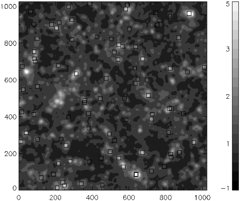
where $\theta_{G}$ is the smoothing angular scale. Figure 1 shows a smoothed $\kappa$-map of $2\times 2\hbox{ deg}^{2}$ with $\theta_{G}=1\hbox{ arcmin}$. The grey-scale indicator shown in the right is in terms of the signal-to-noise ratio explained in the next section. The squares denote dark matter halos found in the corresponding directions with mass $M\geq 10^{14}h^{-1}\hbox{ M}_{\odot}$. Qualitatively, we do see good associations between peaks in the $\kappa$-map and massive dark matter halos.

To identify a match between a peak and a halo quantitatively, we adopt the algorithm of Hamana et al. (2004). Specifically, the matching is carried out in two directions: whether a peak has a corresponding halo and whether a halo has an associated peak in the $\kappa$-map. Because it is not expected that the position of a peak coincides exactly with the central position of its corresponding halo, the matched pair candidate is searched within a radius of $2.88\hbox{ arcmin}$ around a peak or the center of a halo. The specific number $2.88\hbox{ arcmin}$ is chosen to be the same as that of Hamana et al. (2004), and it corresponds to $24$ pixels in our $\kappa$ maps. The closest one is identified as the primary match. Then there are five different peak-halo matching classes: double primary match, missing halo, false peak, secondary peak and secondary halo. A peak-halo pair is classified as a double primary match if both the peak and the halo are their corresponding primary matches. A missing halo is that there is no matched peak in the searching area around the halo. A false peak is that there is no associated halo around the peak. If a halo has a matched peak that has its own primary matched halo, this halo is classified as a secondary halo. A secondary peak has an associated halo, but is not the primary peak of that halo (Hamana et al. 2004). Our investigation focuses on the class of double primary match.

We do $2\times 2\hbox{ deg}^{2}$ surveys toward $720$ directions for each simulation run. Of them, we discard those that have nearby halos ($z<0.1$) more massive than $5\times 10^{13}h^{-1}\hbox{ M}_{\odot}$. The final number of surveys used in our analysis is $428$, $487$, and $401$ for the three simulations, respectively.

3 Results

3.1 NFW density profiles

The NFW density profile of a dark matter halo is described by

$$\rho(x)=\frac{\rho_{s}}{(r/r_{s})(1+r/r_{s})^{2}},$$ (4)

where $r_{s}$ and $\rho_{s}$ are the characteristic scale and density of the halo, respectively. Given the virial mass $M_{vir}$ of the halo, $r_{s}$ can be calculated through the fitting formula

$$c_{n}={c_{n*}\over 1+z}\bigg{(}{M\over 10^{14}h^{-1}M_{\odot}}\bigg{)}^{-0.13},$$ (5)

where the concentration parameter $c_{n}=r_{vir}/r_{s}$ with $r_{vir}$ the virial radius of the halo, and $c_{n*}=8$ for the cosmological model considered here. Then $\rho_{s}$ can be obtained by

$$M_{vir}={4\pi\rho_{s}r_{vir}^{3}\over c_{n}^{3}}\bigg{[}\log(1+c_{n})-{c_{n}\over 1+c_{n}}\bigg{]}.$$ (6)

Thus the density profile of a halo is fully determined by its mass. Cutting off the mass distribution of a halo at its virial radius, the surface mass density can be written as (e.g., Hamana et al. 2004)

$$\Sigma(x)=2\rho_{s}r_{s}f(x),$$ (7)

where $x=r/r_{s}$ and

$$f(x)=\left\{\begin{array}[]{ll}{\sqrt{c_{n}^{2}-x^{2}}\over(x^{2}-1)(1+c_{n})}+{1\over(1-x^{2})^{3/2}}\hbox{arccosh}{x^{2}+c_{n}\over x(1+c_{n})},&\hbox{(x$<$1),}\\ {\sqrt{c_{n}^{2}-1}\over 3(1+c_{n})}\bigg{(}1+{1\over 1+c_{n}}\bigg{)},&\hbox{(x$=$1),}\\ {\sqrt{c_{n}^{2}-x^{2}}\over(x^{2}-1)(1+c_{n})}+{1\over(1-x^{2})^{3/2}}\hbox{arccos}{x^{2}+c_{n}\over x(1+c_{n})},&\hbox{ (1$<$ x$\leq$ $c_{n}$),}\\ 0,&\hbox{(x$>$ $c_{n}$)}.\end{array}\right.$$ (8)

The convergence $\kappa$ is then

$$\kappa={\Sigma(x)\over\Sigma_{cr}}=\kappa_{s}f(x),$$ (9)

where

$$\Sigma_{cr}={c^{2}\over 4\pi G}{D_{s}\over D_{d}D_{ds}},$$ (10)

with $D_{s}$, $D_{d}$ and $D_{ds}$ are the angular diameter distances to the source, to the lens, and from the lens to the source, respectively, and

$$\kappa_{s}=2\rho_{s}r_{s}\Sigma_{cr}^{-1}.$$ (11)

Then one can obtain the smoothed central $\kappa$ from a dark matter halo by

$$\kappa_{0}=\int 2\pi\kappa(\theta/\theta_{s})W_{G}(\theta,\theta_{G})\theta d\theta.$$ (12)

Thus for a NFW spherical dark matter halo, there is a one-to-one correspondence between its $\kappa_{0}$ and its mass $M_{vir}$.

We consider double-primary-matched halo-peak pairs. For each halo, from its mass and redshift, we calculate the expected $\kappa_{0NFW}$, and compare it with the real $\kappa$ value of the corresponding peak. Similar to other studies (e.g., White et al. 2002; Hamana et al. 2004), we use the signal-to-noise ratio $\nu=\kappa_{0}/\sigma_{noise}$ to represent the height of a peak with $\sigma_{noise}$ given by

$$\sigma_{noise}^{2}={\sigma_{\epsilon}^{2}\over 2}{1\over 2\pi\theta_{G}^{2}n_{g}},$$ (13)

where $\sigma_{\epsilon}$ is the rms of the intrinsic ellipticity of source galaxies, $n_{g}$ is the surface number density of source galaxies. Following Hamana et al. (2004), we take $\sigma_{\epsilon}=0.4$ and $n_{g}=30\hbox{ arcmin}^{-2}$. In most of our analyses, we use $\theta_{G}=1\hbox{ arcmin}$. The corresponding $\sigma_{noise}=0.02$. For a typical cluster of $M\sim 10^{14}\hbox{M}_{\odot}$, the peak $\kappa\sim 0.1$ and thus $\nu\sim 5$ for $\theta_{G}=1\hbox{ arcmin}$. Therefore it is appropriate to choose $\theta_{G}$ in the $arcmin$ scale for clusters of galaxies (Hamana et al. 2004). To illustrate the effect of using a different $\theta_{G}$, we will also present results with $\theta_{G}=2\hbox{ arcmin}$, in which $\sigma_{noise}=0.005$.

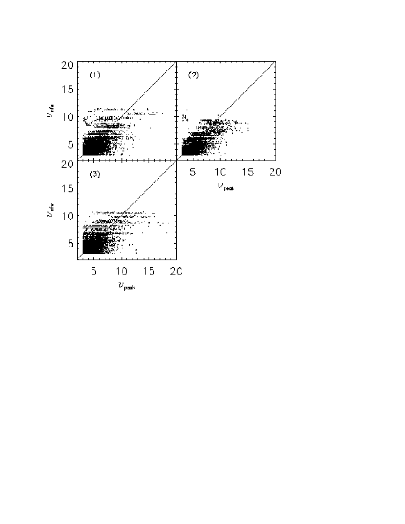
In Figure 2, we show the scatter plots of $\nu_{NFW}$ and $\nu_{peak}$ for the three simulation runs, where $\nu_{NFW}$ stands for the expected central signal-to-noise value for a halo modeled as a spherical NFW one, and $\nu_{peak}$ is the halo’s matched peak value from $\kappa$-maps. We only consider halos with $M\geq 5\times 10^{13}h^{-1}\hbox{ M}_{\odot}$ and peaks with $\nu_{peak}\geq 3$. From the plots, we do see a correlation between $\nu_{NFW}$ and $\nu_{peak}$, but the dispersion is rather large. Quantitatively, we find that the dispersion $\sigma\sim 1.2,1.3$, and $1.4$ for $\nu_{NFW}=4.5,5$ and $6$, respectively. We also note that the average $\nu_{NFW}-\nu_{peak}$ is slightly off zero, with $\nu_{NFW}-\nu_{peak}\sim-0.3$. Hamana et al. (2004) found a positive bias with $\nu_{NFW}-\nu_{peak}\sim 0.24$. It is likely that the small bias arises from simulation to simulation variances. On the other hand, the large dispersion indicates that for a cosmological model, the lensing-selected cluster abundance can deviate significantly from that predicted based on the spherical NFW description of cluster profiles. Therefore the NFW approximation can introduce large systematic errors in extracting cosmological parameters from lensing cluster surveys.

3.2 Triaxial dark matter halos

After a rough calculation, Hamana et al. (2004) attributed the dispersion to the statistical distribution of the concentration parameter of the NFW density profile, and the projection effects of uncorrelated structures along the line of sight. Here we will study in detail the reasons of the dispersion, with particular attention paid to the triaxiality of dark matter halos.

With high resolution simulations, Jing and Suto (2002) present a NFW-like triaxial density profile for dark matter halos, which is given by

$$\rho(R)=\frac{\rho_{cr}(z)\delta_{ce}}{(R/R_{0})^{\alpha}(1+R/R_{0})^{3-\alpha}},$$ (14)

where $\rho_{cr}(z)$ is the critical matter density of the universe at redshift $z$ and

$$R^{2}=\frac{x^{\prime 2}}{c_{x}^{2}}+\frac{y^{\prime 2}}{c_{y}^{2}}+z^{{\prime}2},$$ (15)

with the axial ratios $c_{x}\leq c_{y}\leq 1$. The characteristic scale $R_{0}$ is related to the triaxial concentration parameter $c_{e}=R_{e}/R_{0}$ with $R_{e}\approx 0.45R_{vir}$ defined in Jing and Suto (2002). Given the mass of a halo, the average $c_{x}$ and $c_{y}$, and $c_{e}$, as well as their statistical distributions are derived explicitly from simulation results (Jing & Suto 2002).

The effects of the triaxiality on strong lensing results, such as arc statistics and the probability of large-separation multiple images, have been studied in detail (e.g., Oguri et al. 2003; Oguri & Keeton 2004). The associated asphericity of the intracluster gas, revealed by X-ray and Sunyaev-Zeldovich effect observations, has also been investigated (e.g., Lee & Suto 2003, 2004; Wang & Fan 2004). Here we analyze the dispersion between $\nu_{peak}$ and $\nu_{NFW}$ caused by the aspherical mass distribution of dark matter halos.

The $\kappa$ profile of a triaxial dark matter halo can be analytically written as (Oguri et al. 2003)

$$\kappa(\zeta)=\frac{2\delta_{ce}\rho_{cr}R_{0}}{\sqrt{g}\Sigma_{cr}}f(\zeta),$$ (16)

where the factor $g$ is defined as

$$g=\sin^{2}\theta(\frac{1}{c_{x}^{2}}\cos^{2}\phi+\frac{1}{c_{y}^{2}}\sin^{2}\phi)+\cos^{2}\theta,$$ (17)

with $(\theta,\phi)$ the polar coordinates of the line-of-sight direction. The factor $f$ is the same as that in equation (8) but with the variable $\zeta$ labeling the elliptical contours of the projected surface mass distribution. Specifically,

$$\zeta^{2}={1\over g}(Ax^{2}+Bxy+Cy^{2}),$$ (18)

where we have assumed that the lensing plane is described by $(x,y)$ coordinates, and

$$A=\cos^{2}\theta\bigg{(}{1\over c_{x}^{2}}\sin^{2}\phi+{1\over c_{y}^{2}}\cos^{2}\phi\bigg{)}+{1\over c_{x}^{2}c_{y}^{2}}\sin^{2}\theta,$$ (19)

$$B=\cos\theta\sin 2\phi\bigg{(}{1\over c_{x}^{2}}-{1\over c_{y}^{2}}\bigg{)},$$ (20)

and

$$C={1\over c_{y}^{2}}\sin^{2}\phi+{1\over c_{x}^{2}}\cos^{2}\phi.$$ (21)

Thus for a triaxial halo of mass $M_{vir}$ at a fixed redshift $z$, its lensing signal depends on the line-of-sight direction. The statistical uncertainties of the axial ratios ($c_{x}$ and $c_{y}$) and of the concentration parameter ($c_{e}$) also contribute to the dispersion of lensing signals.

To demonstrate the dispersion caused by different viewing directions, in Figure 3 we show the simulation result (solid line) of the distribution of the associated peak $\nu$ values of a halo of $M=3.9\times 10^{14}h^{-1}\hbox{M}_{\odot}$ at $z=0.48$ viewed along different line of sights. Also shown in the plot (dashed line) is the smoothed central $\nu$ distribution expected from a triaxial halo of this mass and redshift with its axial ratios determined from the real mass distribution of the halo. The concentration parameter $c_{e}$ is taken to be the average value (Jing & Suto 2002). It is seen that the lensing signal has a large dispersion, and the triaxial model does explain a large portion of it at high end.

We now analyze the distribution of $\nu$ expected from the triaxial model for a given $\nu_{NFW}$. Because $\nu_{NFW}$ depends both on the mass and on the redshift of a halo, halos of different masses at different redshifts can have same $\nu_{NFW}$. Thus the conditional distribution is

$$f(\nu)=p(\nu|\nu_{NFW})=\frac{\int_{0}^{1}dz\frac{dV}{dzd\Omega}n[M_{\rm vir}(\nu_{NFW},z),z]p\,[\nu|\nu_{NFW};M_{\rm vir}(\nu_{NFW},z),z]dz}{\int_{0}^{1}dz\frac{dV}{dzd\Omega}n[M_{\rm vir}(\nu_{NFW},z),z]},$$ (22)

where $n(M_{\rm vir},z)$ is the mass function of dark matter halos. The probability function $p[\nu|\nu_{NFW};M_{\rm vir}(\nu_{NFW},z),z]$ depends on the distributions of $\theta$, $\phi$, $c_{x}$, $c_{y}$ and $c_{e}$. Specifically,

$$p[\nu|\nu_{NFW};M_{\rm vir}(\nu_{NFW},z),z]d\nu= \bigg{\{}\int dc_{x}\int d(c_{x}/c_{y})\int dc_{e}\int d\theta\bigg{(}{\partial\nu\over\partial\phi}\bigg{)}^{-1}_{\theta,c_{x},c_{x}/c_{y},c_{e}}$$ (23)

$$p(c_{x})p[(c_{x}/c_{y})|c_{x}]p(c_{e})p(\theta)p(\phi)\bigg{\}}d\nu$$

where the distributions on $c_{x}$, $c_{x}/c_{y}$, and $c_{e}$ are taken from Jing and Suto (2002) [see also Oguri et al. (2003; 2004)]. The mass function of Jenkins et al. (2001) is adopted.

In Figure 4, we show the $\nu$ distribution for $\nu_{NFW}=4.5,5$ and $6$, respectively. The solid lines are the results from $\kappa$ maps of three simulation runs. The dashed lines are the results of equation (22). The dash-dotted lines are the results for spherical halos taking into account the uncertainties of the concentration parameter. It is clearly seen that the dispersion solely from the distribution of the concentration parameter (dash-dotted lines) is small in comparison with the large dispersion shown in simulation data (solid lines). The triaxiality contributes additional dispersions, giving rise to a long tail at high $\nu$ side.

The high-end dispersion due to the triaxiality of dark matter halos has important effects on modeling the selection function for weak lensing cluster surveys. Since the lensing signal from a triaxial cluster depends not only on its mass and redshift but also on the viewing direction, the selection criteria corresponding to a detection limit $\kappa_{lim}$ is no longer simply a mass limit $M_{lim}(z)$ for each redshift $z$. Instead, for each $M_{vir}$, there is a probability $p(M_{vir},z;\kappa_{lim})$ that its $\kappa$ can be higher than $\kappa_{lim}$. Eq.(23) is the basic equation to obtain $p(M_{vir},z;\kappa_{lim})$. One of our future studies is to analyze $p(M_{vir},z;\kappa_{lim})$ and further the weak lensing cluster abundances at different redshifts for different cosmologies.

It is seen from Figure 4 that the triaxial model explains the dispersion better for more massive clusters. It is notably seen, however, that the range of $\nu$ from simulations is broader than that predicted by the triaxial model, especially at the low end of $\nu$. For relatively weak detections ($\nu_{NFW}=4.5$), the differences between the results from the model predictions and the simulations show up at both low and high $\nu$ values. Possible reasons for these are discussed in the following.

The differences between the simulation results and the triaxial model predictions can be attributed to two effects. One is the complex mass distribution of individual clusters that cannot be well approximated by the triaxial model. The other is the projection effect of uncorrelated structures along the line of sight. To see the relative importance of the two, we generate lensing surveys for matched halos only. Specifically, only particles that belong to the matched halos are kept and all the other particles are removed from the simulation. In this way, we isolate the effect of the complexity of individual clusters. The lensing signal from this artificial survey is referred to as $\kappa_{single}$ (or equivalently $\nu_{single}$).

Figure 5 shows the scatter plots of $\nu_{single}$ vs. $\nu_{peak}$ for $\nu_{NFW}=4.5,5$ and $6$, respectively, where $\nu_{peak}$ is the peak $\nu$ value of matched halos from full simulations. Good correlations between the two are clearly seen. This association indicates that for these peaks, their $\kappa$ values are dominantly determined by the properties of their matched halos. The plots also reveal that the dispersion toward high $\nu_{peak}$ is larger for smaller halos (lower $\nu_{NFW}$). This shows, as expected, that the line-of-sight projection effects are relatively stronger for smaller halos. Quantitatively, we calculate the quantity $<[(\nu_{peak}-\nu_{single})/\nu_{single}]^{2}>^{1/2}$ to estimate the strength of the projection effect. The values are $0.25$, $0.18$ and $0.15$ for $\nu_{NFW}=4.5,5$ and $6$, respectively. In the plots, the triangles denote clusters with more than one $\nu$ peak associated with them. These clusters must contain large substructures. Note that we identify the $\nu$ peak closest to the central position of a halo as its matched peak. For clusters with large substructures, the closest $\nu$ peak is likely generated only by a substructure. Thus the value of matched $\nu_{peak}$ underestimates the lensing signal from the full cluster. We indeed see that the triangles concentrate on the small $\nu_{peak}$ part. This explains the lower-end extension of the distribution of $\nu_{peak}$ in Figure 4.

Now let us compare $\nu_{single}$ with $\nu_{tri}$ calculated from the triaxial model in which we determine the axial ratios and the orientation of a cluster from its real mass distribution. The results are shown in Figure 6. The symbols are the same as in Figure 5. First we do see correlations between $\nu_{single}$ and $\nu_{tri}$, with the associations better for single-peak clusters (crosses). It is noted, however, that the triaxial model predicts narrower scatters than $\nu_{single}$ for relatively small clusters. For large clusters with $\nu_{NFW}=6$, the spread of $\nu_{tri}$ is about the same as that of $\nu_{single}$. Secondly, as expected, most of the triangles are in the lower right part of the plot. But there are several triangles scattered at the upper left part. We check individual cases, and find that multiple substructures along the line of sight can produce a higher lensing signal than that predicted by the smoothed triaxial mass distribution.

We caution that the simulations we use are relatively small-sized ($100h^{-1}\hbox{ Mpc}$), and the number of large clusters is small. As we stack simulation boxes together to generate lensing maps, the same cluster can be surveyed many times along different directions. For $\nu_{NFW}=4.5,5$, and $6$, the number of matched peaks from lensing maps is, respectively, about $400$, $300$, and $200$. However, the corresponding total number of clusters involved in our analyses is only $26,23$ and $14$. The number of times that the most frequently surveyed clusters appear in our lensing maps can account for about $25\%$ of the total number of matched peaks. Thus our statistical results can be influenced significantly by the characteristics of only a few clusters. Similar analyses on larger simulations are desired for more robust statistical results.

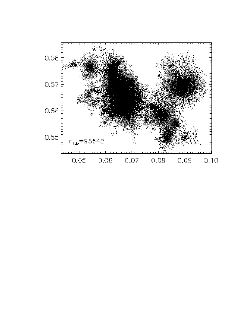
We further do case-studies one by one. Of the respective $26,23$ and $14$ clusters for $\nu_{NFW}=4.5,5$, and $6$, the number of clusters with apparent substructures shown in lensing maps is $11,12$ and $10$, with the corresponding fraction $42\%$, $52\%$ and $71\%$. For these clusters, their lensing signals are mostly lower than those predicted by the triaxial model as explained earlier. A specific example is plotted in Figure 7. The $z$-projected mass distribution of this cluster is shown in Figure 8. Large subhalos are clearly seen. In fact, in this case, the cluster is in its early formation stage, and different substructures are just starting to merge. For those clusters without apparent substructures, most of them can be well described by the triaxial model. However, multiple hidden substructures along the line of sight can generate lensing signals higher than those from the smoothed triaxial model. An example is shown in Figure 9. For this cluster, the expected lensing signal from the spherical NFW mass distribution is $\nu_{NFW}=6$. Taking into account the triaxiality of the mass distribution, the predicted lensing signals largely agree with that calculated directly from the real mass distribution of the cluster. For the extreme point where $\nu_{single}$ is much higher than $\nu_{tri}$, the mass distribution along this particular line of sight is shown in Figure 10. The upper panel is the real distribution and the lower one is from the smoothed triaxial model. Multiple major peaks are clearly seen in the upper panel, which explains the deviation of $\nu_{single}$ from $\nu_{tri}$. Notice that when applying the triaxial model to individual clusters, we adopt the mean concentration parameter from Jing and Suto (2002) for a given set of axial ratios measured from the mass distribution of a cluster. The real concentration parameter can fluctuate around the mean. We do find that, in a few cases ($5$ or $6$ out of $23$ clusters with $\nu_{NFW}=5$), the real mass distribution is much flatter than that of the triaxial model with the mean concentration parameter, which results higher $\nu_{single}$ than $\nu_{tri}$.

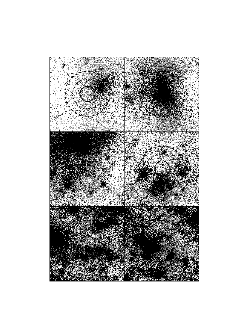
The above analyses were done for the smoothing radius $\theta_{G}=1\hbox{ arcmin}$. To see the effects of $\theta_{G}$, we also perform studies with $\theta_{G}=2\hbox{ arcmin}$. Figure 11 shows the dispersions for $\theta_{G}=2\hbox{ arcmin}$. Only the results from simulations (solid lines) and from the triaxial model (dashed lines) are shown. It is seen that the differences between the simulation results and the predictions of the triaxial model are larger than those for $\theta_{G}=1\hbox{ arcmin}$. Quantitatively, for $\theta_{G}=1\hbox{ arcmin}$ and $\nu_{NFW}=6$, the dispersions are $\sigma_{simu}\approx 1.5$ and $\sigma_{tri}\approx 0.9$, respectively. The corresponding numbers for $\theta_{G}=2\hbox{ arcmin}$ are $\sigma_{simu}\approx 1.8$ and $\sigma_{tri}\approx 0.6$. In Figure 12, we show the scatter plots of $\nu_{single}$ and $\nu_{peak}$. First, as expected, the fraction of triangles is significantly less than that of $\theta_{G}=1\hbox{ arcmin}$. For $\theta_{G}=2\hbox{ arcmin}$, the fraction is $9\%$, $19\%$ and $11\%$ for $\nu_{NFW}=4.5$, $5$, and $6$, respectively. For $\theta_{G}=1\hbox{ arcmin}$, the corresponding numbers are $23\%$, $32\%$, and $38\%$. The decrease of the effect of substructures does not however reduce significantly the dispersion of $\nu_{peak}$ at low end for $\theta_{G}=2\hbox{ arcmin}$. Secondly, the correlations of the two can still be seen in Figure 12, but the tightness of the association is worse than the case of $\theta_{G}=1\hbox{ arcmin}$. For $\theta_{G}=2\hbox{ arcmin}$ and $\nu_{NFW}=6$, we have $\sigma[(\nu_{single}-\nu_{peak})/\nu_{single}]\approx 0.24$. For $\theta_{G}=1\hbox{ arcmin}$, $\sigma[(\nu_{single}-\nu_{peak})/\nu_{single}]\approx 0.15$. The large dispersion reflects the severe projection contamination for $\theta_{G}=2\hbox{ arcmin}$. In Figure 13, we show the particle distribution at several lens planes for a particular peak with $\nu_{peak}=4.5$. This peak appears in both cases of $\theta_{G}=1\hbox{ arcmin}$ and $\theta_{G}=2\hbox{ arcmin}$. The corresponding primary cluster of the peak is located at plane $11$. The three circles in each panel are for angular scales of $1\hbox{ arcmin}$, $2\hbox{ arcmin}$ and $3\hbox{ arcmin}$, respectively. It is clearly seen that within the circle of $1\hbox{ arcmin}$, the cluster itself is the dominant contributor to the lensing effect, and the projection effect from other planes is relatively weak. Within the circle of $2\hbox{ arcmin}$, however, besides the cluster, the mass distribution on planes $7,13,31,33$ and $39$ contributes significantly to the final lensing effect. Specifically, $(\nu_{peak}-\nu_{single})/\nu_{single}\approx 0.37$ and $0.8$ for $\theta_{G}=1\hbox{ arcmin}$ and $\theta_{G}=2\hbox{ arcmin}$, respectively. We note that the projection effect causes large dispersions at both high and low ends. The joint effects of the stronger projection contamination and the reduction of substructures make the low-end dispersion not change greatly in comparison with that of $\theta_{G}=1\hbox{ arcmin}$. At the high end, however, the dispersion is significantly larger for $\theta_{G}=2\hbox{ arcmin}$ than for $\theta_{G}=1\hbox{ arcmin}$. Thus our analysis indicates that it seems too large to use $\theta_{G}=2\hbox{ arcmin}$ in weak lensing cluster surveys.

4 Discussion

Our study shows that for clusters of galaxies, their peak lensing signals appear much more complex than those predicted by the spherical mass distribution in which the total mass and the redshift of a cluster fully determine the strength of its lensing effects. Therefore the spherical model can introduce large errors to the prediction on the abundance of lensing-selected clusters. Those errors in turn will significantly bias the determination of cosmological parameters from future weak lensing cluster surveys.

Hamana et al. (2004) attribute the complexity to the variation of the concentration parameter of the spherical NFW profile and the line-of-sight projection effect of uncorrelated structures. However, our analyses with $\theta_{G}=1\hbox{ arcmin}$ reveal that for relatively large clusters relevant to weak lensing cluster surveys, their lensing effects are mainly determined by the characteristics of individual clusters, and the line-of-sight projection effects play a minor role. For individual clusters, the triaxiality of their mass distribution is important and has to be taken into account in theoretical analyses on their expected lensing effects. In terms of the dispersion shown in Figure 4, the triaxiality contributes a considerable part of the high-end tail especially for massive clusters. The low-end extension is mainly attributed to the existence of large substructures in clusters of galaxies. Multiple substructures along a line of sight can also generate higher lensing signals than those predicted by the smoothed mass distribution. Thus substructures also contribute, to a certain level, to the high-end dispersion. With $\theta_{G}=2\hbox{ arcmin}$, however, the projection effect is significant. Thus in terms of cluster detections with weak lensing surveys, the smoothing radius $\theta_{G}=1\hbox{ arcmin}$ is preferable to $\theta_{G}=2\hbox{ arcmin}$.

Note that our analyses are based on the $\kappa$ maps generated under the Born approximation. Therefore we may underestimate the projection effect because we integrate the weighted density fluctuations along the unperturbed light path. In our analysis with $\theta_{G}=1\hbox{ arcmin}$, we find that the projection effect accounts for about $0.16$ in the total dispersion of $\sim 1.39$ of $\nu_{peak}-\nu_{NFW}$ for $\nu_{NFW}=5$. Hamana et al. (2004) quoted a value of $\sim 0.5$ from the projection effect estimated from the contribution of large-scale structures uncorrelated with halos (Hoekstra 2001). While the number $0.5$ is not certain and the underestimate by the Born approximation in the weak lensing limit may not be as large as the numbers ($0.16$ vs. $0.5$) suggest, it is indeed desirable to quantitatively analyze the projection effects by full ray tracing simulations.

In our analysis, we assume a fixed source redshift. For a real lensing survey, source galaxies generally have a redshift distribution, which should be taken into account in modeling the lensing effects of clusters expected from the survey.

With the mass distribution and the statistics for the triaxial dark matter halos from Jing and Suto (2002), the effect of the triaxiality on lensing signals can be theoretically studied. Rather than simply mass selected, a much more complicated selection function for $\kappa$-limited lensing cluster surveys can be obtained. On the other hand, it is less straightforward to include substructures in theoretical analyses without numerical simulations. However, recent high resolution simulations have been able to present some statistics on substructures, e.g., their mass function and the spatial distribution (e.g. Gao et al. 2004; Natarajan & Springel 2004). These, in principle, allow us to analyze the influence of substructures on lensing effects without time-intensive simulations.

Weak lensing effects are powerful and clean probes to the distribution of dark matter. Cosmological studies on lensing-selected clusters avoid physical processes related to the intracluster gas that complicate the cosmological applications of X-ray and SZ-selected clusters considerably. Our investigation reveals the complexities of lensing effects related to the mass distribution of clusters, which however, can be handled without fundamental difficulties. In a foreseeable future, weak lensing cluster surveys as well as cosmic shear observations will contribute greatly to cosmological studies.

Figure 1: A $2^{o}\times 2^{o}$ $\kappa$-map from a simulation.

Figure 2: Scatter plots of $\nu_{peak}$ vs. $\nu_{NFW}$ for the three simulation runs, respectively.

Figure 3: The distribution of $\nu$ for a particular cluster with $M\approx 3.9\times 10^{14}h^{-1}\hbox{M}_{\odot}$ at redshift $z=0.48$ ($\nu_{NFW}=6$) viewed from different directions. The dashed line is the Monte-Carlo result of the triaxial model for all the possible line-of-sight directions. The axial ratios are calculated from the mass distribution of the cluster. The solid line is the result from simulations.

Figure 4: The distribution of $\nu$ for all the clusters with $\nu_{NFW}=4.5,5$ and $6$, respectively. The solid line is the result from $\kappa$ maps, the dashed line is the statistical result from the triaxial model, and the dash-dotted line is the result of shperical NFW model taking into account the statistical variation of the concentration parameter.

Figure 5: Scatter plots of $\nu_{peak}$ vs. $\nu_{single}$. The three plots are for $\nu_{NFW}=4.5,5$ and $6$, respectively. The triangles denote cases that multiple $\kappa_{single}$ peaks appear within $2.88\hbox{ arcmin}$ around the center of the clusters. The crosses are for those that only one $\kappa_{single}$ peak exists within $2.88\hbox{ arcmin}$ around the center of the clusters.

Figure 6: Scatter plots of $\nu_{tri}$ vs. $\nu_{single}$. The symbols are the same as in Fig5.

Figure 7: The scatter plot of $\nu_{tri}$ vs. $\nu_{single}$ for a particular cluster ’95645’ with $\nu_{NFW}=6$.

Figure 8: The projected particle distribution along $z$-direction for cluster ’95645’.

Figure 9: The scatter plot of $\nu_{tri}$ vs. $\nu_{single}$ for a particular cluster ’71218’ with $\nu_{NFW}=6$.

Figure 10: The mass density along the line-of-sight direction corresponding to the highest point in Fig.9. The upper panel is the real mass distribution of the cluster, and the lower panel is the one from the smoothed triaxial mass distribution.

Figure 11: Same as Figure 4 but with $\theta_{G}=2\hbox{ arcmin}$. Solid lines are results from simulations and dashed lines are the predictions from the triaxial model.

Figure 12: Same as Figure 5 but with $\theta_{G}=2\hbox{ arcmin}$.

Figure 13: The particle distribution in lens planes $7,11,13,31,33$ and $39$ for a particular peak with $\nu_{peak}=4.5$. The three circles from inner most to the outer most correspond to angular scales of $1\hbox{ arcmin}$, $2\hbox{ arcmin}$ and $3\hbox{ arcmin}$, respectively.

References

- Bahcall & Bode (2003) Bahcall, N., & Bode, P. 2003, ApJ, 588, L1
- Bartelmann & Meneghetti (2004) Bartelmann, M., & Meneghetti, M. 2004, A&A, 418, 413
- Bartelmann & Schneider (2001) Bartelmann, M., & Schneider, P. 2001, Phys. Rept. 340, 291
- (4) Carlstrom, J. E., Holder, G. P., & Reese, E. D., 2002, ARA&A, 40, 643
- Fan & Chiueh (2001) Fan, Z. H., & Chiueh, T. H. 2001, ApJ, 550, 547
- Fan & Wu (2003) Fan, Z. H., & Wu, Y. L. 2003, ApJ, 598, 713
- Gao et al. (2004) Gao, L., White, S. D. M., Jenkins, A., Stoehr, F., & Springel, V. 2004, MNRAS, 355, 819
- Gavazzi et al. (2003) Gavazzi, R., Fort, B., Mellier, Y., Pello, R., & Dantel-Fort, M. 2003, A&A, 403, 11
- Haiman, Mohr & Holder (2001) Haiman, Z., Mohr, J., & Holder, G. 2001, ApJ, 553, 545
- Haiman et al. (2004) Haiman, Z., Wang, S., Hennawi, J. F., May, M., Spergel, D.N., & Tyson, J. A. 2004, American Astronomical Society Meeting 205, #108.15
- Hamana, Colombi & Mellier (2001) Hamana, T., Colombi, S., & Mellier, Y. 2001, in XXXVth Moriond Astrophysics Meeting: Cosmological Physics with Gravitational Lensing. ed. J.-P. Kneib, Y. Mellier, M. Mon, & T. Tran Thanh Van(France: EDP)
- Hamana, Takada & Yoshida (2004) Hamana, T., Takada, M., & Yoshida, N. 2004, MNRAS, 350, 893
- Hoekstra (2001) Hoekstra, H. 2001, A&A, 370, 743
- (14) Jain, B., Seljak, U., & White, S. 2000, ApJ, 530, 547
- (15) Jenkins, A. et al. 2001, MNRAS, 321, 372
- Jing & Suto (1998) Jing, Y. P., & Suto, Y. 1998, ApJ, 494, L5
- Jing, & Suto (2002) Jing, Y. P., & Suto, Y. 2002, ApJ, 574, 538
- Jing (2004) Jing, Y. P. 2004, private communication
- Kaiser (1998) Kaiser, N. 1998, ApJ, 498, 26
- Lee & Suto (2003) Lee, J., & Suto, Y. 2003, ApJ, 585, 151
- Lee & Suto (2004) Lee, J., & Suto, Y. 2004, ApJ, 601, 599
- Ma (2003) Ma, C. P. 2003, ApJ, 584, L1
- Natarajan & Springel (2004) Natarajan, P., & Springel, V. 2004, ApJ, 617, 13L
- Oguri, Lee & Suto (2003) Oguir, M., Lee, J., & Suto, Y. 2003, ApJ, 599, 70
- Oguri, Lee & Suto (2004) Oguir, M., Lee, J., & Suto, Y. 2004, ApJ, 608, 1175
- Oguri & Keeton (2004) Oguri, M., & Keeton, C. 2004, ApJ, 610, 6630
- Padmanabhan, Seljak & Pen (2003) Padmanabhan, N., Seljak, U., & Pen, U. L. 2003, New Astronomy, 8, 581
- Press & Schechter (1974) Press, W. H., & Schechter, P. 1974, ApJ, 187, 425
- Reblinsky & Bartelmann (1999) Reblinsky, K., & Bartelmann, M. 1999, A&A, 345, 1
- (30) Rosati, P., Borgani, S., & Norman, C. 2002, ARA&A, 40, 539
- (31) Sheth, R., & Tormen, G. 1999, MNRAS, 308, 119
- Tereno, Dore, vanWaerbeke & Mellier (2005) Tereno, I., Dore, O., van Waerbeke, L., & Mellier, Y. 2005, A&A, 429, 383
- vanWaerbeke (2000) van Waerbeke, L. 2000, MNRAS, 313, 524
- vanWaerbeke, Mellier & Hoekstra (2005) van Waerbeke, L., Mellier, Y., & Hoekstra, H. 2005, A&A, 429, 75
- Wang & Fan (2004) Wang, Y.-G., & Fan, Z.H. 2004, ApJ, 617, 847
- White, vanWaerbeke & Mackey (2002) White, M., van Waerbeke, L., & Mackey, J. 2002, ApJ, 575, 640
- Zhang (2004) Zhang, T. J. 2004, ApJ, 602, L5