The Fourth VLBA Calibrator Survey — VCS4

Abstract

This paper presents the fourth extension to the Very Long Baseline Array (VLBA) Calibrator Survey, containing 258 new sources not previously observed with very long baseline interferometry (VLBI). This survey, based on three 24 hour VLBA observing sessions, fills remaining areas on the sky above declination $-40\arcdeg\$ where the calibrator density is less than one source within a 4° radius disk at any given direction. The share of these area was reduced from 4.6% to 1.9%. Source positions were derived from astrometric analysis of group delays determined at 2.3 and 8.6 GHz frequency bands using the Calc/Solve software package. The VCS4 catalogue of source positions, plots of correlated flux density versus projected baseline length, contour plots and fits files of naturally weighted CLEAN images, as well as calibrated visibility function files are available on the Web at http://gemini.gsfc.nasa.gov/vcs4.

1. Introduction

This work is a continuation of the project of surveying the sky for bright compact radio sources. These sources can be used as phase referencing calibrators for imaging of weak objects with very long baseline interferometry (VLBI) and as targets for space navigation, monitoring the Earth’s rotation, differential astrometry and space geodesy. The method of VLBI, first proposed by Matveenko et al. (1965), allows us to determine positions of sources with nanoradian precision (1 nrad $\approx$ 0.2 mas). Several catalogues were compiled combining observations under various programs. The catalogue of sources observed under geodetic programs from 1979 through 2004, ICRF-Ext2 (Fey et al. 2004), contains positions of 776 sources. In addition to that, positions of 2247 sources were determined in the framework of the VLBA Calibrator Survey project: VCS1 (Beasley et al. 2002), VCS2 (Fomalont et al. 2003) and VCS3 (Petrov et al. 2005). Since 364 sources are listed in both the ICRF-Ext2 and the VCS catalogues, the total number of sources for which positions were determined with VLBI is 2659. Among them, 2269 sources, or 85%, are considered as acceptable calibrators: they had at least 8 successful observations at both X and S bands and the semi-major axis of the error ellipse of their coordinates is less than 25 nrad (5 mas).

However, the sky coverage of these sources is not uniform. Successful phase referencing requires a calibrator within at least 4° from a target source with a precise position and known source structure. The probability of finding a calibrator from the combined ICRF-Ext2, VCS1, VCS2 and VCS3 catalogues within 4° of any target above $-40\arcdeg\$ is 95.4%. In this paper we present an extension of the VCS catalogues, called the VCS4 catalogue, mainly concentrating on the other 4.6% of the sky where the source density is the lowest and on the brightest sources with flat spectrum previously not observed with VLBI under geodesy and astrometry programs. Since the observations, calibrations, astrometric solutions and imaging are similar to that of VCS1–3, most of the details are described by Beasley et al. (2002) and Petrov et al. (2005). In section §2 we assess an a priori probability of source detection. In section §3 we describe the strategy for selecting 412 candidate sources observed in three 24 hour sessions with the very long baseline array (VLBA) based on analysis of probabilities of source detection which is a further development of the statistical approach for source selection introduced by Petrov et al. (2005). In section §4 we briefly outline the observations and data processing. We present the catalogue in §5, and summarize our results in §6.

2. Assessment of an a priori probability of source detection

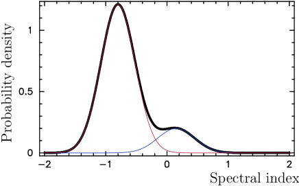
Having unlimited resources one could try to observe all sources stronger than some limiting flux density. However, only sources with bright compact components can be detected with VLBI and may be useful for phase referencing or geodetic applications. Kellermann, Pauliny-Toth, & Davis (1968) first showed that the distribution of sources over spectral index $\alpha\enskip(F\propto\nu^{+\alpha})$ has two peaks: one near $\alpha=-1$ (steep spectrum) and another near $\alpha=0$ (flat spectrum). Later, it was confirmed that extended objects dominate in the steep spectrum population (see the review by Kellermann & Owen 1988). In compact regions, which have the synchrotron mechanism of emission, the peak in the spectrum caused by synchrotron self-absorption has frequencies higher than 1 GHz due to their small size (Slysh 1963). Thus, if the dominating emission comes from compact regions, the spectrum of the total flux density will be predominantly flat or inverted.

Let’s determine the probability of detecting with the VLBA a source with a given total flux density and given spectral index. The empirical probability distribution function of sources in spectral indexes can be approximated as

$$P(\alpha)=(1-a)\,N(\alpha,\alpha_{\mathrm{s}},\sigma_{\mathrm{s}})\,+\,a\,N(\alpha,\alpha_{\mathrm{f}},\sigma_{\mathrm{f}})\,,$$ (1)

where $a$ is the fraction of the flat-source population to the total population, $N(\alpha,\alpha_{o},\sigma_{o})$ is the normal distribution with maximum at $\alpha_{o}$ and dispersion $\sigma_{o}^{2}$. The first term $N_{\mathrm{s}}(\alpha)=N(\alpha,\alpha_{\mathrm{s}},\sigma_{\mathrm{s}})$ represents the probability distribution for steep spectrum sources, the second one $N_{\mathrm{f}}(\alpha)=N(\alpha,\alpha_{\mathrm{f}},\sigma_{\mathrm{f}})$ — for flat spectrum sources. Using results of Mingaliev et al. (2001) for the RATAN–600 simultaneous broad-band spectra survey at centimeter wavelengths of sources around the North Celestial Pole, as well as 2.7 & 5 GHz data from Wright & Otrupcek (1990) PKSCat90 catalog with limiting flux density at 2.7 GHz of 250 mJy, we have found the following estimates of distribution parameters: $a=0.15$, $\sigma_{\mathrm{f}}=0.30$, $\alpha_{\mathrm{f}}=0.15$, $\sigma_{\mathrm{s}}=0.28$, $\alpha_{\mathrm{s}}=0.80$. Figure 1 shows the distribution.

Figure 1.— The probability density distribution at 8.6 GHz as a function of spectral index. The thin lines show the distribution of the steep spectrum source population (left) and the flat spectrum the source population (right).

If a source has a spectral index in the range of $[\alpha,\alpha+d\alpha]$, the ratio of the probability that it belongs to the flat spectrum population, $P_{\mathrm{f}}(\alpha)$, to the probability that it belongs to the steep spectrum population, $P_{\mathrm{s}}(\alpha)$, is equal to the ratio of their probability densities:

$$\frac{\displaystyle P_{\mathrm{f}}(\alpha)}{\displaystyle P_{\mathrm{s}}(\alpha)}=\frac{\displaystyle a\,N_{\mathrm{f}}(\alpha)}{\displaystyle(1-a)\,N_{\mathrm{s}}(\alpha)}\,.$$ (2)

Since we assume that a source either belongs to the flat spectrum population or to the steep spectrum population, $P_{\mathrm{f}}(\alpha)+P_{\mathrm{s}}(\alpha)=1$. Then we immediately find

$$P_{\mathrm{f}}(\alpha)=\frac{\displaystyle a\,N_{\mathrm{f}}(\alpha)}{\displaystyle(1-a)\,N_{\mathrm{s}}(\alpha)+a\,N_{\mathrm{f}}(\alpha)}\,,\vspace{2ex}$$ (3)

$$P_{\mathrm{s}}(\alpha)=\frac{\displaystyle(1-a)\,N_{\mathrm{s}}(\alpha)}{\displaystyle(1-a)\,N_{\mathrm{s}}(\alpha)+a\,N_{\mathrm{f}}(\alpha)}\,.$$ (4)

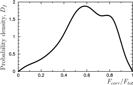
The probability that a given source will have a ratio $r$ of the correlated flux density $F_{corr}$ to the total flux density $F_{tot}$ is quite different for these two populations. Results of Kovalev et al. (2005) of the 2 cm VLBA survey (Kellermann et al. 1998) and results of analysis of the VCS3 observing campaign provided us estimates of $F_{corr}$ at baseline projections equal to the Earth radius. The total flux of these sources was measured with the RATAN–600. The histogram over 500 sources after smoothing and normalization gives us an estimate of the empirical probability density distribution of the ratio of correlated flux density at baseline projections equal to the Earth radius to the total flux density among the flat spectrum source population (figure 2).

Figure 2.— The probability density distribution at 8.6 GHz of the ratio of the correlated flux density at the baseline projections equal to the Earth radius to the total flux density among the flat spectrum source population.

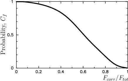
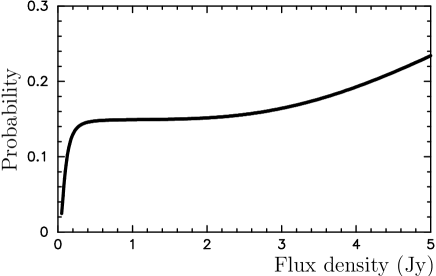
According to our previous experience in processing snapshot VLBA Calibrator survey observations with integration time 4 minutes and bit rate 128 Msamples/sec with good weather conditions, sources with correlated flux density greater than 60 mJy are reliably detected. We set the detection limit of the VLBA to $F_{lim}$ = 70 mJy in order to have a little allowance for possible pointing errors and higher than normal system temperature due to bad weather. The probability to have the correlated flux density greater than this limit, $F_{lim}$, i.e. the probability of detection for a source which belongs to the flat spectrum population and has total flux density $F_{tot}$ is $\rho_{\mathrm{f}}(F_{tot})=C_{\mathrm{f}}\biggl{(}\frac{\displaystyle F_{lim}}{\displaystyle F_{tot}}\biggr{)}$ where $C_{f}(r)$ is the cumulative probability function defined as

$$C_{\mathrm{f}}(r)=1-\int\limits_{0}^{r}D_{\mathrm{f}}(r)\,dr\,,$$ (5)

and where $D_{f}(r)$ is the probability distribution function of the ratio of the correlated flux density to the total flux density and $r$ is the ratio of minimal detected correlated flux density to total flux density. The plot of $D_{\mathrm{f}}(r)$ is shown in figure 2 and plot of $C_{\mathrm{f}}(r)$ is shown in figure 3.

Figure 3.— The cumulative probability function of the ratio of the correlated flux density to the total flux density among the flat spectrum source population: $C_{f}(r,F_{corr}/F_{tot})=P_{f}(r\leq F_{corr}/F_{tot})$.

For steep spectrum sources the probability density function of the ratio of the correlated flux density to the total flux density is not well known. According to our analysis of compact steep spectrum sources detected in VCS1–3 experiments, we approximate

$$D_{\mathrm{s}}(r)=\cases{20,&\mbox{if} \enskip$r<0.05$\,,\cr\hphantom{2}0,&\mbox{if} \enskip$r\geq 0.05$\,.\cr}$$ (6)

Analogously, we introduce the function $C_{\mathrm{s}}(r)$ for the steep spectrum source population:

$$C_{\mathrm{s}}(r)=1-\int\limits_{0}^{r}D_{\mathrm{s}}(r)\,dr\,.$$ (7)

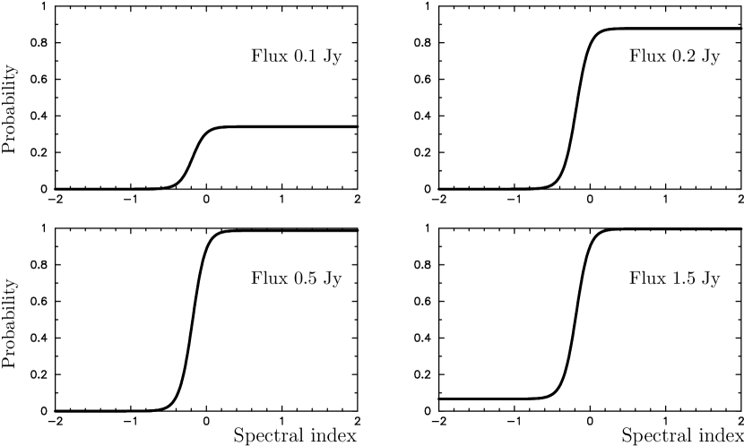
Then, assuming the spectral index of a source is precisely known, the probability to be detected at 8.6 GHz for a source with spectral index $\alpha$ and total flux density $F_{o}$ measured at frequency $f_{o}$ is

$$P(F_{o},f_{o},\alpha)=P_{\mathrm{f}}(\alpha)\,C_{\mathrm{f}}\biggl{(}\frac{F_{lim}}{F_{o}+(8.6/f_{o})^{\alpha}}\biggr{)}+$$

$$P_{\mathrm{s}}(\alpha)\,C_{\mathrm{s}}\biggl{(}\frac{F_{lim}}{F_{o}+(8.6/f_{o})^{\alpha}}\biggr{)}\,.\hphantom{\,.}$$ (8)

Plots of the probability of being detected as a function of spectral index are presented in figure 4.

If no information about the spectral index is available, the estimate of the probability to detect a source is (see figure 5)

$$P(F_{o})=\int\limits_{-\infty}^{+\infty}\left(P_{\mathrm{f}}(\alpha)\,C_{\mathrm{f}}\biggl{(}\frac{F_{lim}}{F_{o}+(8.6/f_{o})^{\alpha}}\biggr{)}+\hphantom{da\,.}\right.$$

$$\left.P_{\mathrm{s}}(\alpha)\,C_{\mathrm{s}}\biggl{(}\frac{F_{lim}}{F_{o}+(8.6/f_{o})^{\alpha}}\biggr{)}\right)\,d\alpha\,.$$ (9)

Figure 4.— Probability of being detected at 8.6 GHz as a function of spectral index for sources with flux density at 1.4 GHz 0.1 Jy, 0.2 Jy, 0.5 Jy and 1.5 Jy.

Figure 5.— The probability of detection of a source with unknown spectral index as a function of total flux density at 1.4 GHz.

3. Selection of candidate sources for zones with low calibrator density

As the first step of source selection we computed the sky source density on a $6^{\prime}\times 6^{\prime}$ grid and identified areas with declination $>-40^{\circ}$ with no calibrator within a $3^{\circ}$ disk.

As the second step we selected all sources from the NVSS catalogue with flux density greater than 100 mJy at 1.4 GHz, with galactic latitude $|b|>1^{\circ}\!.5$ which either were not previously observed with VLBI under astrometry and geodesy programs, or which were observed, but did not collect enough data in order to be counted as calibrators. We used the CATS database (Verkhodanov et al. 1997) to gather all available flux density measurements and then computed a spectral index for each source. Sources with spectral index less than $-0.5$ were deselected. We also deselected sources with extrapolated total flux density at 8.6 GHz less than 100 mJy. Sources for which the spectral index could not be reliably determined were removed from the list of candidates if they had flux densities at 1.4 GHz less than 200 mJy. We also removed pairs of sources if the distance between components was less than $0^{\circ}\!.083$, since it usually indicates a source with extended structure. Those sources, which according to NASA Extragalactic Database (NED), were listed as galactic objects, H II regions or planetary nebulae, were removed as well. Finally, we generated the input list of 2479 candidates. For 1216 objects we had estimates of their spectral indexes, and we computed a priori probability of their detection using expression (8). For other sources we computed this probability using expression (9). It should be mentioned that many sources have variable flux density and spectral index. These variations were not taken into account in evaluation of the probability distribution and equation (8). This makes the estimates of the probability of detection somewhat less reliable.

If all these sources could be observed, the mathematical expectation of the area without a calibrator within a disk with radius of $4^{\circ}$ would be 0.57%. For economical reasons we were forced to reduce the list of candidates. In order to find a subset of $N$ sources in such a manner that the area with the source calibrator density less than one source in a disk with radius $4^{\circ}$ would be minimal, we adopted the following iterative procedure. Initially, we selected all sources. For each point on the grid with declination $>-40^{\circ},$ which before the VCS4 campaign had no calibrators closer than $4^{\circ}$, we computed the probability of that that point will have no calibrator closer than $4^{\circ}$ after VCS4 observations as

$$H_{ij}=\>\prod\limits_{k=1}^{k=n}(1-P_{i}(\alpha,F))\>d(i,j,k)\,,$$ (10)

where $d(i,j,k)$ is 1, if the distance between the point on the grid $(i,j)$ and the $k$th source is less than $4^{\circ}$, and 0 otherwise. The sum

$$R=\sum\limits_{grid}H_{ij}$$ (11)

is the mathematical expectation of the total area which has no calibrator within $4^{\circ}$.

Then at each step of iteration for each source we compute $R_{k}=\displaystyle\sum\limits_{grid}\mbox{$R\>d(i,j,k)$}\,/\,\mbox{$(1-P_{i}(\alpha,F))$}$, i.e., the contribution of the $k$th source to $R$. The source with the minimal contribution is removed, the probability $H_{ij}$ is updated, and the procedure is repeated until $N$ source remained in the list.

We generated the final list of candidates by concatenating two lists: 1) a list of 300 sources selected according to the iterative process described above; 2) a list of 100 sources north of declination $-30^{\circ}$ with the highest probability of detection — these are the strongest flat spectrum sources previously not observed in geodetic VLBI mode. We also added 12 sources which had been previously observed and detected under geodetic programs, but never imaged with the VLBA. Of them, 5 sources fell in the areas with no calibrators, and therefore were considered as belonging to list 1, the other 7 sources were added to list 2. The mathematical expectation of the area which would remain with no calibrator after observing the final list of 412 objects was 1.77%.

The rational for including the list of the one hundred brightest sources was that the area of the sky without a calibrator within a disk with radius $4^{\circ}$ is reduced too slowly with an increase in the number of candidates beyond several hundred. For most geodetic applications having a bright calibrator a little bit further from the target is more important than having a calibrator closer, but much weaker. On the other hand, for accurate phase referencing, a relatively close weak calibrator is often preferable to a stronger calibrator which is much further away. So, some compromise is needed in order to improve the calibrator list.

4. Observations and data processing

The VCS4 observations were carried out in three 24 hour observing sessions with the VLBA on 2005 May 12, 2005 June 12, and 2005 June 30. Each target source was observed in two scans. The scan duration was 120 seconds for sources from the list of 107 bright objects, and 235 seconds for other target sources. The target sources were observed in a sequence designed to minimize loss of time from antenna slewing. In addition to these objects, 93 strong sources were taken from the GSFC astrometric and geodetic catalogue 2004f_astro. Observations of 3–4 strong sources from this list were made every 1–1.5 hours during observing sessions. These observations were scheduled in such a way, that at each VLBA station at least one of these sources was observed at an elevation angle less than 20°, and at least one at an elevation angle greater than 50°. The purpose of these observations was to provide calibration for mismodeled atmospheric path delays and to tie the VCS4 source positions to the ICRF catalogue (Ma et al. 1998). The list of troposphere calibrators was selected among the sources which according to the 2cm survey results (Kovalev et al. 2005) showed the greatest compactness index, i.e. the ratio of the flux density of an unresolved detail to the total flux density at VLBA baselines. In total, 505 sources were observed. The antennas were on-source 60% of the time.

Similar to the previous VLBA Calibrator Survey observing campaign (Petrov et al. 2005), we used the VLBA dual-frequency geodetic mode, observing simultaneously at 2.3 GHz and 8.6 GHz. Each band was separated into four 8 MHz channels (IFs) which spanned 140 MHz at 2.3 GHz and 490 MHz at 8.6 GHz, in order to provide precise measurements of group delays for astrometric processing. Since the a priori coordinates of candidates were expected to have errors of up to 30″, the data were correlated with an accumulation period of 1 second in 64 frequency channels in order to provide extra-wide windows for fringe searching.

Processing of the VLBA correlator output was done in three steps. In the first step the data were calibrated and fringed using the Astronomical Image Processing System (AIPS) (Greisen 1988). In the second step data were imported to the Caltech DIFMAP package (Shepherd 1997) and images were produced using the optimized automated procedure originally suggested by Greg Taylor (Pearson et al. 1994). We were able to reach the VLBA image thermal noise level for most of our CLEAN images (Wrobel & Ulvestad 2005). Errors of our estimates of correlated flux density of sources brighter than 100 mJy are determined mainly by the accuracy of amplitude calibration, which for the VLBA, according to Wrobel & Ulvestad (2005), is at the level of 5% at 1–10 GHz. This estimate was confirmed by comparison of the correlated flux density with the single-dish flux density which we measured with RATAN–600 in March 2005 for slowly varying sources without extended structure. The methods of single-dish observations and data processing can be found in Kovalev et al. (1999). In the third step, the data were imported to the Calc/Solve software, group delays ambiguities were resolved, outliers eliminated and coordinates of new sources were adjusted using ionosphere-free combinations of X band and S band group delay observables of the 3 VCS4 sessions, 15 VCS1–3 experiments and 3976 twenty four hour International VLBI Service for astrometry and geodesy (IVS) experiments in a single least square solution. The boundary conditions which require zero net-rotation of new coordinates of the 212 sources listed as defined in the ICRF catalogue with the respect to their positions from that catalogue were imposed in order to select a unique solution of differential equations of photon propagation.

In a separate solution, coordinates of the 93 well known tropospheric calibrators were estimated from the VCS4 observing sessions only. Comparison of estimates of coordinates of these sources with coordinates derived from analysis of 3976 twenty four hour IVS experiments provided us a measure of the accuracy of coordinates from the VCS4 observing campaign. The differences in coordinate estimates were used for computation of parameters $a$ and $b(\delta)$ of error inflation model in the form of $\sqrt{(a\,\sigma)^{2}+b(\delta)^{2}}$, where $\sigma$ is an uncertainty derived from the fringe amplitude signal to noise ratio using the error propagation law and $\delta$ is declination. More details about analysis and imaging procedure can be found in Beasley et al. (2002) and Petrov et al. (2005). The histogram of source position errors is presented in Figure 6.

Figure 6.— Histogram of semi-major error ellipse of position errors. The last bin shows errors exceeding 9 mas.

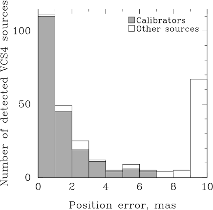
In total, 292 out of 412 sources were detected and yielded at least two good points for position determination. However, not all of these sources are suitable as phase referencing calibrators or as targets for geodetic observations. Following Petrov et al. (2005) we consider a source suitable as a calibrator if 1) the number of good X/S pairs of observations is 8 or greater in order to rule out the possibility of a group delay ambiguity resolution error; and 2) position error before reweighting is less than 5 mas following the strategy adopted in processing VCS observations. Only 196 sources satisfy this calibrator criteria. It should be mentioned that our criterion for suitability as a phase calibrator is rather conservative, and sources which fail this criterion may still be useful for some applications. Among 292 detected sources, 34 were previously observed but did not have enough observations before the VCS4 campaigns to be considered as calibrators. Of these 34 objects, new VCS4 observations of 27 of them provided enough information to classify them as calibrators.

Table 1 shows statistics of the a priori and a posteriori detection rate. The a priori probability gives us a reasonable estimate of the detection rate. The sources from list 1 are weaker than the sources from list 2, and for 40% of them the integration time of 4 minutes was insufficient to qualify them as calibrators. The a posteriori detection rate turned out greater than the a priori rate, because we set the detection limit to 70 mJy when computing the a priori detection rate. In fact, we were able to detect sources with correlated flux density as low as 50 mJy with integration time 4 minutes.

Table 1 The number of observed and detected sources

Data	# sources	# detections	# calibrators	detection rate		calibrators
				a priori	a posteriori
List 1	305	199	117	45 %	65 %	38 %
List 2	107	93	82	84 %	87 %	77 %
Total	412	292	199	57 %	71 %	48 %

a

Figure 7.— From top to bottom. Naturally weighted CLEAN images at S-band (2.3 GHz). The lowest contour levels (2 steps) on images are plotted at “clev” levels (Jy/beam), the peak brightness — “max” values (Jy/beam). The dashed contours indicate negative flux. The beam is shown in the bottom left corner of the images. Dependence of the correlated flux density at S-band versus projected spacings. The error bars were computed on the basis of correlated flux density scatter around mean value. Naturally weighted CLEAN images at X-band (8.6 GHz). Dependence of the correlated flux density at X-band versus projected spacings.

5. The VCS4 catalogue

Table 2The VCS4 catalogue

	Source name		J2000.0 Coordinates		Errors (mas)				Correlated flux density (Jy)
									8.6 GHz		2.3 GHz
Class	IVS	IAU	Right ascension	Declination	$\Delta\alpha$	$\Delta\delta$	Corr	# Obs	Total	Unres	Total	Unres	Band
(1)	(2)	(3)	(4)	(5)	(6)	(7)	(8)	(9)	(10)	(11)	(12)	(13)	(14)
$-$	0006$-$363	J0008$-$3601	00 08 33.661411	$-$36 01 25.05213	6.20	32.64	0.697	8	$0.07$	$\cdots$	$0.22$	0.10	X/S
C	0010$+$336	J0012$+$3353	00 12 47.382197	$+$33 53 38.47157	0.58	0.84	$-$0.508	41	$0.16$	0.13	$0.07$	0.06	X/S
C	0012$+$319	J0015$+$3216	00 15 06.147414	$+$32 16 13.30953	0.33	0.55	$-$0.211	86	$0.20$	0.11	$0.13$	0.09	X/S
C	0021$-$084	J0024$-$0811	00 24 00.672734	$-$08 11 10.04881	1.08	2.13	$-$0.252	31	$0.10$	0.08	$0.09$	0.07	X/S
C	0024$-$114	J0026$-$1112	00 26 51.443027	$-$11 12 52.42503	0.96	1.68	0.219	30	$0.11$	0.05	$0.19$	0.09	X/S
C	0032$+$612	J0035$+$6130	00 35 25.310617	$+$61 30 30.76144	0.93	0.60	0.200	71	$0.14$	0.06	$0.23$	0.07	X/S
$-$	0033$-$088	J0035$-$0835	00 35 46.250383	$-$08 35 54.04258	0.83	1.57	$-$0.240	86	$0.13$	0.12	$0.06$	0.06	X
C	0052$-$201	J0054$-$1953	00 54 32.948443	$-$19 53 01.00202	0.42	0.83	$-$0.091	59	$0.16$	0.10	$0.20$	0.05	X/S
C	0052$-$125	J0055$-$1217	00 55 11.782596	$-$12 17 57.09709	0.25	0.46	$-$0.220	90	$0.24$	0.18	$0.21$	0.15	X/S
$-$	0057$+$101	J0059$+$1022	00 59 46.769108	$+$10 22 40.42531	16.93	17.91	0.797	2	$\cdots$	$\cdots$	$\cdots$	$\cdots$	S

Note. — Table 2 is presented in its entirety in the electronic edition of the Astronomical Journal. A portion is shown here for guidance regarding its form and contents. Units of right ascension are hours, minutes and seconds, units of declination are degrees, minutes and seconds.

The VCS4 catalogue is listed in Table 2. The first column gives source class: “C” if the source can be used as a calibrator, “–” if it cannot. The second and third columns give IVS source name (B1950 notation), and IAU name (J2000 notation). The fourth and fifth columns give source coordinates at the J2000.0 epoch. Columns /6/ and /7/ give inflated source position uncertainties in right ascension and declination (without $\cos\delta$ factor) in mas, and column /8/ gives the correlation coefficient between the errors in right ascension and declination. The number of group delays used for position determination is listed in column /9/. Columns /10/ and /12/ give the estimate of the flux density integrated over entire map in Jansky at X and S band respectively. This estimate is computed as a sum of all CLEAN components if a CLEAN image was produced. If we did not have enough detections of visibility function to produce a reliable image, the integrated flux density is estimated as the median of the correlated flux density measured at projected spacings less than 25 and 7 M$\lambda$ for X and S bands respectively. The integrated flux density has a meaning of the source total flux density with spatial frequencies less than 4 M$\lambda$ at X band and 1 M$\lambda$ at S band filtered out, or by another words this is the flux density from all details of a source with size less than 50 mas at X band and 200 mas at S band. Column /11/ and /13/ give the flux density of unresolved components estimated as the median of correlated flux density values measured at projected spacings greater than 170 M$\lambda$ for X band and greater than 45 M$\lambda$ for S band. For some sources no estimates of the integrated and/or unresolved flux density are presented, because either no data were collected at the baselines used in calculations, or these data were unreliable. Column /14/ gives the data type used for position estimation: X/S stands for ionosphere-free linear combination of X and S wide-band group delays; X stands for X band only group delays; and S stands for S band only group delays. Some sources which yielded less than 8 pairs of X and S band group delay observables had 2 or more observations at X and/or S band observations. For these sources either X-band or S-band only estimates of coordinates are listed in the VCS4 catalogue, whichever uncertainty is less.

            

Figure 8.— Source sky density before (left) and after (right) the VCS4 observing campaign. The area above $-40\arcdeg\$ declination with calibrator source density less than one source within a 4° radius disk is shown in black.

In addition to this table, the html version of this catalogue is posted on the Web. For each source it has 8 links: to a pair of postscript maps of the source at X and S-band; to a pair of plots of correlated flux density as a function of the length of the baseline projection to the source plane; to a pair of fits files with CLEAN components of naturally weighted source images; and to a pair of fits files with calibrated $uv$ data. The coordinates and the plots are also accessible from the NRAO VLBA Calibration Search web-page.

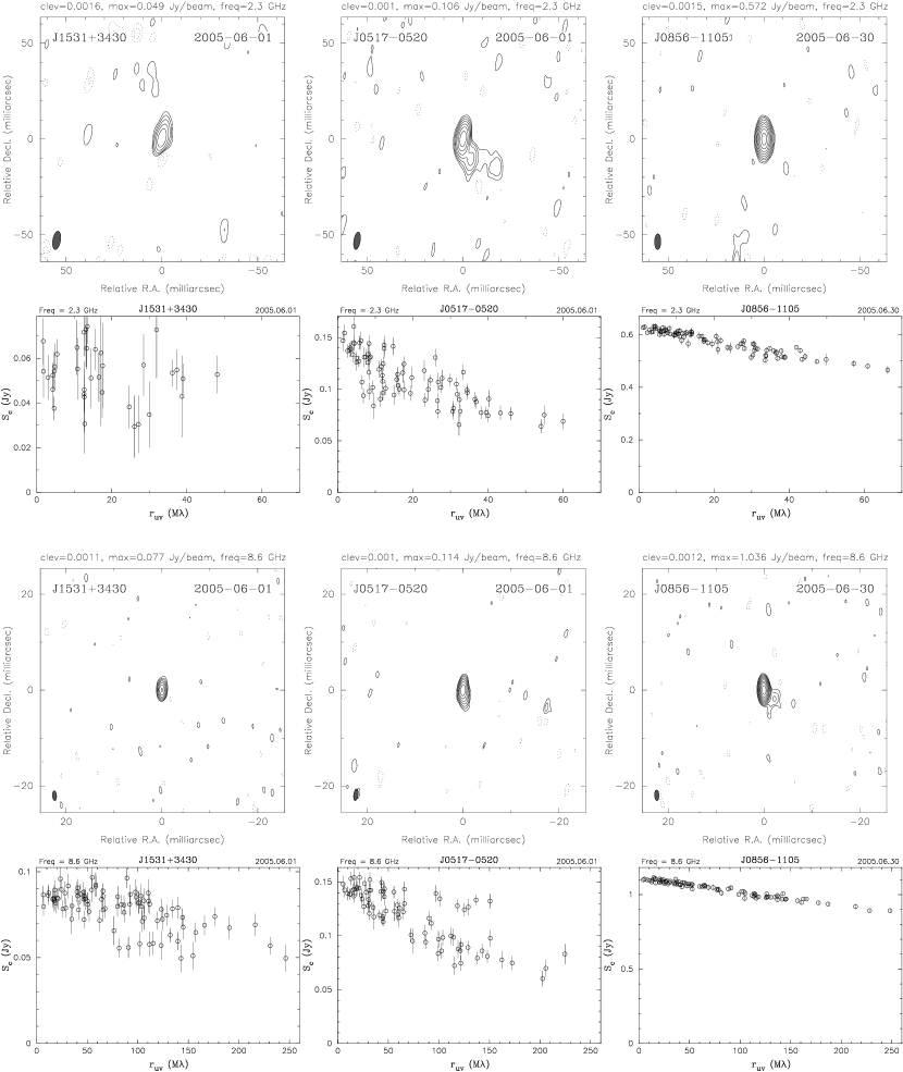
Figure 7 presents examples of naturally weighted contour CLEAN images as well as estimates of the correlated flux density versus projected spacings. The S band data for the source J1531+3430 is an example of one of the weakest sources which we still were able to image. It turned out to be an object with an inverted radio spectrum of the milliarcsecond emission. The images of J0517-0520 show the compact structure with jet components which were detected on the level of several mJy/beam only. The source J0856-1105 has the highest VLBI flux density at X band among all the new VCS4 objects and will be useful for geodetic applications along with a few tens of other compact VCS4 objects with high flux density at VLBA baselines.

6. Summary

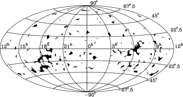
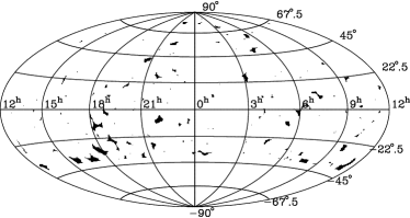
The VCS4 Survey has added 258 new sources not previously observed with VLBI. Among of them, 199 sources turned out to be suitable as phase referencing calibrators and as target sources for geodetic applications. The area with source density less than one calibrator within a disk of radius $4^{\circ}$ in any given direction on the sky with $\delta>-40^{\circ}$ was reduced from 4.6 % to 1.9 % (refer to figure 8 and table 3). After processing the VCS4 experiments, the total number of calibrators has grown from 2268 to 2472. This pool of calibrators was formed from analysis of 18 VLBI Calibrator Survey and 3976 twenty four hour IVS astrometry and geodesy observing sessions.

The strategy of source selection based on a priori probabilities of source detection developed in this study was successful. The conservative a priori estimate of detection rate was 57%, while the a posteriori detection rate is 70 %. The a priori estimate of the area with the calibrator density less than one object within a disk of radius $4^{\circ}$ was 1.8 %, while the a posteriori value is 1.9 %.

Table 3 The probability to find a calibrator at any given direction within a circle of a given radius in selected declination zones.

Search circle	Declination zone
radius	[$-90^{\circ}$, $-40^{\circ}]$	[$-40^{\circ}$, $-30^{\circ}]$	[$-30^{\circ}$, $+90^{\circ}]$
$4^{\circ}\!.0$	63.6 %mm	92.2 %mm	98.6 %mm
$3^{\circ}\!.5$	55.4 %mm	86.0 %mm	96.0 %mm
$3^{\circ}\!.0$	44.1 %mm	76.4 %mm	89.7 %mm
$2^{\circ}\!.5$	33.2 %mm	56.6 %mm	77.9 %mm
$2^{\circ}\!.0$	22.7 %mm	46.6 %mm	60.7 %mm
$1^{\circ}\!.5$	13.6 %mm	29.4 %mm	40.0 %mm
$1^{\circ}\!.0$	6.3 %mm	14.2 %mm	20.1 %mm
$0^{\circ}\!.5$	1.6 %mm	3.7 %mm	5.4 %mm

The sky calibrator density for different radii of a search circle and for three different declination zones is presented in table 3. A further search for new calibrators to decrease the area with insufficient sky calibrator density would be considerably less efficient, because the majority of the flat spectrum sources in those areas have already been observed. The remaining sources are the steep spectrum sources, or sources with unknown spectral index, or very weak objects. According to figure 5 the lack of information about spectral index of potential candidates makes the detection rate of almost any sample about the same.

At the same time, some relatively bright flat spectrum sources remained in the zones where there is at least one calibrator in a disk with radius $4^{\circ}$. A sample of 675 such sources was observed in July 2005 with the VLBA in a follow-up VCS5 experiment (Y.Y. Kovalev et al. in preparation). The addition of these sources to the VLBA Calibrator list will not affect the calibrator sky density with the search radius of $4^{\circ}$, but will increase the density of calibrators with smaller search circles, which will be beneficial for many applications, for instance, the VERA project (Honma et al. 2003).

New VCS4 detected sources were observed in 2005 with the Russian Academy of Sciences 600 meter ring radio telescope RATAN for measurement of their instantaneous 1–22 GHz spectra (Y.Y. Kovalev et al. in preparation). These data will allow us to determine compactness of these sources and their accurate spectral indexes. Using this information one can further improve the estimate of the a priori probability of source detection with VLBI as a function of source flux and spectral index which is essential for source selection in future surveys.

References

- Beasley et al. (2002) Beasley, A. J., Gordon, D., Peck, A. B., Petrov, L., MacMillan, D. S., Fomalont, E. B., & Ma, C. 2002, ApJS, 141, 13
- Fomalont et al. (2003) Fomalont, E., Petrov, L., McMillan, D. S., Gordon, D., Ma, C. 2003, AJ, 126, 2562
- Fürst et al. (1990) Fürst, E., Reich, W., Reich, P., & Reif, K. 1990, A&AS, 85, 805
- Greisen (1988) Greisen, E. W., 1988, in Acquisition, Processing and Archiving of Astronomical Images, ed. G. Longo & G. Sedmak (Napoli: Osservatorio Astronomico di Capodimonte), 125
- Honma et al. (2003) Honma, M., Fujii, T., Hirota, T., Horiai, K., Iwadate, K., Jike, T., Kameya, O., Kamohara, R., Kan-Ya, Y., Kawaguchi, N., Kobayashi, H., Kuji, S., Kurayama, T., Manabe, S., Miyaji, T., Nakashima, K., Omodaka, T., Oyama, T., Sakai, S., Sakakibara, S.-I., Sato, K., Sasao, T., Shibata, K. M., Shimizu, R., Suda, H., Tamura, Y., Ujihara, H., & Yoshimura, A. 2003, PASJ, 55, L57
- Jackson et al. (2002) Jackson, C. A., Wall, J. V., Shaver, P. A., Kellermann, K. I., Hook, I. M., & Hawkins, M. R. S. 2002, A&A, 386, 97
- Kellermann, Pauliny-Toth, & Davis (1968) Kellermann, K. I., Pauliny-Toth, I. I. K., & Davis, M. M. 1968, Astrophysical Letters, 2, 105
- Kellermann & Owen (1988) Kellermann, K. I. & Owen, F. N. 1988, Galactic and Extragalactic Radio Astronomy, ed. by G. L. Verschur & K. I. Kellermann (Springer Verlag), 563
- Kellermann et al. (1998) Kellermann, K. I., Vermeulen, R. C., Zensus J. A., & Cohen M. H. 1998, AJ, 115, 1295
- Kovalev et al. (1999) Kovalev, Y. Y., Nizhelsky, N. A., Kovalev, Yu. A., Berlin, A. B., Zhekanis, G. V., Mingaliev, M. G., & Bogdantsov, A. V. 1999, A&AS, 139, 545
- Kovalev et al. (2005) Kovalev, Y. Y., Kellermann, K. I., Lister, M. L., Homan, D. C., Vermeulen, R. C., Cohen, M. H., Ros, E., Kadler, M., Lobanov, A. P., Zensus, J. A., Kardashev, N. S., Gurvits, L. I., Aller, M. F., & Aller, H. D. 2005, AJ, 130, in press (astro-ph/0505536)
- Ma et al. (1998) Ma, C., Arias, E. F., Eubanks, T. M., Fey, A. L., Gontier, A.-M., Jacobs, C. S., Sovers, O. J., Archinal, B. A., & Charlot, P., 1998, AJ, 116, 516
- Fey et al. (2004) Fey, A.L., Ma, C., Arias, E. F., Charlot, P., Feissel-Vernier, M., Gontier, A.-M., Jacobs, C. S., Li, J., MacMillan, D. S. 2004, AJ, 127, 3587.
- Matveenko et al. (1965) Matveenko, L. I., Kardashev, N. S., & Sholomitskii, G. B. 1965, Izvestia VUZov. Radiofizika, 8, 651 (English transl. Soviet Radiophys., 8, 461)
- Mingaliev et al. (2001) Mingaliev, M. G., Stolyarov, V. A., Davies, R. D., Melhuish, S. J., Bursov, N. A., & Zhekanis, G. V. 2001, A&A, 370, 78
- Pearson et al. (1994) Pearson, T. J., Shepherd, M. C., Taylor, G. B., & Myers, S. T. 1994, BAAS, 185, 0808
- Petrov et al. (2005) Petrov, L., Kovalev, Y.Y., Fomalont, E., Gordon, D. 2005, AJ, 129, 1163.
- Slysh (1963) Slysh, V.I. 1963, Nature, 199, 682
- Verkhodanov et al. (1997) Verkhodanov, O. V., Trushkin, S. A., Andernach, H., & Chernenkov, V. N. 1997, in ASP Conf. Ser. 125, Astronomical Data Analysis Software and Systems VI, ed. by G. Hunt, & H. E. Payne (San Francisco: ASP), 322
- Shepherd (1997) Shepherd, M. C. 1997, in ASP Conf. Series. 125, Astronomical Data Analysis Software and Systems VI, ed. by G. Hunt & H. E. Payne (San Francisco: ASP), 77
- Winn, Patnaik, & Wrobel (2003) Winn, J. N., Patnaik, A. R., & Wrobel, J. M. 2003, ApJS, 145, 83
- Wright & Otrupcek (1990) Wright, A. E., & Otrupcek, R. 1990, PKSCAT90 Radio Source Catalogue and Sky Atlas (Epping: Australia Telesc. Natl. Facility)
- Wrobel & Ulvestad (2005) Wrobel, J. M. & Ulvestad, J. S. 2004, VLBA status summary, NRAO