ROTSE observations of the young cluster IC 348

Abstract

CCD observations of stars in the young cluster IC 348 were obtained from 2004 August to 2005 January with a 0.45 m ROTSEIIId robotic reflecting telescope at the Turkish National Observatory site, Bakırlıtepe, Turkey. The timing analysis of selected stars whose X-Ray counterpart were detected by Chandra X-Ray Observatory were studied. The time series of stars were searched for rotational periodicity by using different period search methods. 35 stars were found to be periodic with periods ranging from 0.74 to 32.3 days. Eighteen of the 35 periodic stars were new detections. Four of the new detections were CTTSs and the others were WTTSs and G type (or unknown spectral class) stars. In this study, we confirmed the stability of rotation periods of TTauri stars. The periods obtained by Cohen et al. and us were different by 1$\%$. We also confirmed the 3.24 h pulsation period of H254 which is a $\delta$ Scuti type star as noted by Ripepi et al. but the other periods detected by them were not found. We examined correlation between X-ray luminosity and rotational period of our sample of TTSs. There is a decline in the rotational period with X-ray luminosity for late type TTSs.

1 Introduction

IC 348 is a young (less than 10Myr) and nearby cluster ( distance 316 pcs) located in the Perseus complex (Lada $\&$ Lada 1995, Trullols $\&$ Jordi 1997, Herbig 1998, Luhman et al. 1998). This cluster has a number of T Tauri stars (Herbig 1954) which are lower mass (lower than 1.5 M_⊙) Pre-Main-Sequence stars. Deep near infrared imaging survey of IC 348 in the J, H and K bands by Lada $\&$ Lada (1995) resulted with 380 NIR sources as probable cluster members. Herbig (1998) made a survey for stars having H_α emission and discovered over 110 emission line stars brighter than R= 19 magnitude. He found the proportion of WTTSs (weak line TTSs with H_α equivalent width below 10Å  and H_α emission can be assumed to be chromospheric origin) to CTTSs (classical TTSs with H_α equivalent width above 10Å  and H_α emission is probably dominated by the accretion of circumstellar material on to the stars) as 58:51. CTTSs exhibit infrared excess and show a varying photometric light curves irregularly. WTTSs show spectroscopic and photometric periodic variability on time scales of days caused by rotational modulation due to magnetic activity. Luhman et al. (1998) performed deep infrared and optical spectroscopy of IC 348 and found that nearly 25$\%$ of stars within the core of IC 348 and younger than 3 Myr exhibits signature of disks in the form of strong H_α.

Herbst et al. (2000) studied the photometry of 150 stars and discovered 19 periodic variables with periods ranging from 2.24 to 16.2 days and masses ranging from 0.35 to 1.1 M_⊙. This variability is caused by the rotation of the surface with large cool spots whose pattern is often stable for many rotation periods. Recently Cohen et al. (2004) presented results based on 5 yr of monitoring this cluster and found that these periodic stars show modulations of their amplitude, mean brightness and light curve shape on time scales of less than one year.

X-ray observations of IC 348 with ROSAT by Preibisch et al. (1996) resulted with detection of 116 X-ray sources. They found probable new cluster members. They suggested that these were presumably weak line T Tauri stars because of their X-ray properties. WTTSs seem to be stronger X-ray emitters than the CTTSs. They could not find any significant correlation between the H_α luminosity and X-ray luminosity indicating that H_α emission is not a chromospheric emission for CTTSs. Preibisch $\&$ Zinnecker (2001) detected 215 X-ray sources with the Advanced CCD Imaging Spectrometer on board the Chandra X-Ray Observatory. 58 of these sources were identified as new cluster members. They did not find significant differences between the X-ray properties of WTTSs and CTTSs. About 80$\%$ of cluster members with masses between 0.15 and 2 M_⊙were identified as visible X-ray sources. The observed X-ray emission was explained as coronal emission for WTTSs. Chandra X-ray detection fraction of the IC 348 cluster was high for spectral types between the late F and M4. In their next study, Preibisch $\&$ Zinnecker (2002) found a tight correlation between X-ray luminosity and H_α luminosity for the WTTSs. They suggested that the chromosphere was heated by X-rays from the overlying corona. The CTTSs did not show such a relation since H_α emission comes mainly from accretion processes. They pointed out that the use of H_α emission as an indicator for circumstellar material had some problems.

The main goal of this study is to find out if there is a variability in the light curve of some cluster members which have X-ray counterparts. We wanted to examine correlation between X-ray luminosity and rotational period of stars in this cluster in order to see whether rotation is an important parameter governing the X-ray emission. We chose some X-ray emission sources which were detected and located by Chandra X-Ray Observatory. We investigated the corresponding optical light curves of these sources obtained by robotic ROTSEIIId telescope in order to search for variability. We also wanted to investigate the observational results for $\delta$ Scuti star H254 which is a member of this cluster. This star was previously detected by Ripepi et al. (2002) and found as a $\delta$ Scuti star. On the basis of observations of Luhman et al. (1998) H254 (L= 31.4 L_⊙ and T_e= 7200 K) is inside the theoretical pulsational instability strip for the PMS stars determined by Marconi and Palla (1998). Ripepi et al. obtained that H254 pulsates with a pulsation frequency of 7.406 $d^{-1}$. This frequency was confirmed in our observations. Ripepi et al. calculated that this star pulsates either in the fundamental mode or in the first overtone. They gave a mass range of 2.3 and 2.6 M_⊙for this star by computing a sequence of linear non-adiabatic models. In the second section the observations and data reduction were discussed. The results and discussion related with the periodic variables in this cluster were given in the section 3. We summarized our results in the last section.

2 Observations and Data reduction

The CCD observations of cluster stars were performed during August, 2004 and January, 2005 with ROTSEIIId robotic reflecting telescope located at the Turkish National Observatory (TUG) site, Bakırlıtepe, Turkey. ROTSEIII telescopes were described in detail by Akerlof et al. (2003). They were designed for fast ($\sim$6 s) responses to Gamma-Ray Burst triggers from satellites such as Swift. It has a 45 cm mirror and operates without filters. It has equipped with a CCD, 2048$\times$2048 pixel, the pixel scale is 3.3 arcsec per pixel for a total field of view 1.^∘85$\times$1.^∘85. A total of about 1800 CCD frames were collected during the observations. Due to the other scheduled observations and atmospheric conditions we obtained 3 - 40 frames at each night with an exposure time of 5 sec. All images were automatically dark- and flat-field corrected as soon as they were exposed. For each corrected image aperture photometry by SExtractor package (Bertin $\&$ Arnouts 1996) were applied using an aperture of 5 pixels in diameter to obtain the instrumental magnitudes. Then these magnitudes were calibrated by comparing all the field stars against USNO A2.0 R-band catalog with a triangle-matching technique. Barycentric corrections were made to the times of each observation by using JPL DE200 ephemerides prior to the timing analysis with the period determination methods.

3 Results and Discussion

3.1 Pulsation period of $\delta$ Scuti star H254

We first attempted to determine the pulsation period of star H254 (spectral type F0, Harris et al. 1954) ($\alpha$=03^h44^m31$.\!\!^{\rm s}$2, $\delta$=+32^∘06^′22$.\!\!^{\prime\prime}$1) using our nearly 150 days of observational data. Ripepi et al. (2002) identified four frequencies for this source by using their eleven days observations. One of these frequencies was at 7.406 $d^{-1}$ which is typical of $\delta$ Scuti type pulsators. They also reported three more frequencies and explained that these were resulted from the long term behavior associated with a daily variation of H254 and partially, with the similar variability in their comparison star H20. We used differential magnitudes which reduces the systematic effects since we are interested in the time series analysis. As a comparison star we chose H89 (see section 3.2) ($\alpha$=03^h44^m21$.\!\!^{\rm s}$0, $\delta$=+32^∘07^′38$.\!\!^{\prime\prime}$7) which has a spectral type F8. Figure 1 shows ROTSEIIId light curve ($\delta$m_R=m_R²⁵⁴-m_R⁸⁹) obtained between the nights of MJD 53232 and MJD 53382. Period of variation in this light curve was determined by using three separate numerical period searching routines. One is Period98 (by Sperl: available at www.astro.univie.ac.at/^∼dsn/). The other two are the method of Scargle (Scargle 1982) and the Clean method (Roberts et al. 1987). These periodograms are essentially discrete Fourier transform of the input time series. To search any periodicity in the differential light curves, we applied these different period search algorithms mentioned above. For analyzing the periodicity in the light curves periodogram provides an approximation to the power spectrum. To be sure about the periodicity we applied these different period finding methods.

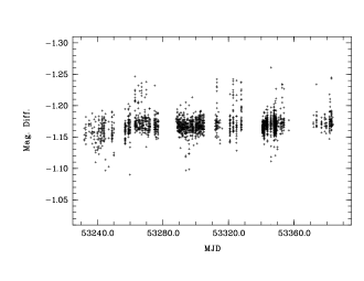
Figure 1: RotseIIId light curve of H254. Error bars on data points are not shown for clarity however estimated errors are of the order $\sim$0$.\!\!^{\rm m}$02

Figure 2 shows the amplitude and power spectra of H254. All of them displays the frequency 7.406 $d^{-1}$. The inset in the first panel shows the window function which is used to describe the response of data analysis system to a perfect sine wave. The peak at one day (and its harmonics) in the periodograms is a signature of nightly windowing of the sampling frequency.

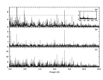
Figure 2: Power spectra for H254. Panel (a): Scargle algoritm, (b): Clean algoritm and (c): Period98. Dotted line on the upper panel represents $3\sigma$ confidence level. Inset is the spectrum of the window function.

For the statistics of periodograms we employed the method of Scargle (Scargle 1982) and evaluated the confidence levels of periodicities. We estimated the noise level of the periodogram by fitting a constant line. The probability of a signal above this level has an exponential probability distribution

$$1-P(Z)=(1-e^{Z})^{N}$$

which is essentially a $\chi^{2}$ distribution for two degrees of freedom. $Z$ is the power at a given frequency and $N$ is the number of frequencies sampled. For given parameters the confidence level of the signal was found. The confidence level of the signal for the maximum power at 7.406 $d^{-1}$ is more than $5\sigma$ level signal detection. As seen from Figure 2a all other detected powers are below the $3\sigma$ detection level which indicate that 0.157, 0.283 and 0.931 $d^{-1}$ frequencies detected by Ripepi et al. (2002) are not present in our light curve. The light curve phased with the frequency 7.406 $d^{-1}$ is shown in Figure 3. The amplitude of pulsation is 4.1 mmag which is comparable with V band amplitude (5.4 mmag) given by Ripepi et al.

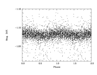
Figure 3: Light curve of H254 phased with the frequency 7.406 d^-1.

The same period was found using two more different comparison stars, H261 (spectral type F2, $\alpha$=03^h44^m24$.\!\!^{\rm s}$6, $\delta$=+32^∘10^′14$.\!\!^{\prime\prime}$4) and H20 (spectral type F8, $\alpha$=03^h43^′58$.\!\!^{\rm s}$1, $\delta$=+32^∘09^′47$.\!\!^{\prime\prime}$5). The amplitude spectra which were obtained by using Clean method are shown in Figure 4. The peak at the frequency 7.406 $d^{-1}$ corresponding to a period of around 3.24 h is seen clearly.

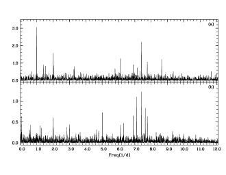
Figure 4: Amplitude spectrum of H254 with other set of reference stars (a) H261 (b) H20.

3.2 Periodic variations in Optical Counterparts of Chandra Sources

In this part of the study we searched for the timing properties of the optical counterparts of selected Chandra X-Ray sources. X-ray images of the cluster IC 348 with the Advanced CCD Imaging Spectrometer on board the Chandra X-Ray observatory were studied by Preibisch $\&$ Zinneker (2001). They determined the positions and count rates of the 215 individual X-ray sources. Identification of the optical counterparts of the X-ray sources with masses 0.15 and 2 M_⊙were performed for 161 X-ray sources.

The positions of Chandra sources whose optical counterparts were identified by Preibisch $\&$ Zinneker (2001) were cross correlated with the positions of ROTSE objects. The main criteria for the selection is 3$.\!\!^{\prime\prime}$3/pixel resolution of the ROTSE CCD frames. Hence, to match a known coordinate 3 pixel (10^′′) diameter aperture is used. Secondly, if there is an object closer than 4 pixels it is rejected. The exposure time is 5 seconds for each frame. This allows us to observe most of the bright stars of IC 348 without overexposing the frames. With this exposure time stars with magnitudes between 10 and 14 are well detected and it is also possible to detect stars upto 17th magnitude depending on atmospheric conditions. For each frame mean FWHM of the point spread function (PSF) is calculated for stars with 10 $>$ m_R $>$ 14 and if the mean FWHM $>$ 2 pixel (6$.\!\!^{\prime\prime}$6) that frame is also rejected. Figure 5a shows the mean of the magnitude measurement errors assigned to each star in finding their mean magnitudes during the whole observation period. For fainter stars the magnitude determining accuracy decreases. The magnitude errors should be excluded from the measured variations in order to obtain the correct intrinsic variabilities. The lower limit for the systematic measurement errors is 0.002 for the brightest star in our figure. For magnitudes of stars $\sim$16 mag, this error is about 0.15 mag. As this error increases with increasing magnitude the measurement of intrinsic variability becomes difficult.

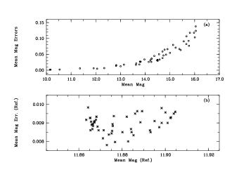
Figure 5: Upper panel shows mean magnitude errors in calculating the mean magnitudes for each star in our sample. The mean magnitude of reference stars and their mean errors for each star under consideration are shown in the lower panel.

3.2.1 Time Series Analysis

To determine any time variability in the selected stars we chose 3 reference (comparison) stars (H89, H20, H139). To select and check stability of the reference stars, we chose a set of stars with variances less than 0.01 mag over the observing interval. Power spectrums of the candidate reference stars were calculated and the ones showing most random power distribution were selected. H89 and H139 from this set was used by Cohen et al. (2004) also. Hence we adopt these stars as the reference stars. Two of these stars have F spectral type and H139 is a G0 star (Luhman et al. 1998). The average magnitude of the selected reference stars were used in the calculation of differential magnitudes. Figure 5b shows the mean magnitudes of the reference stars obtained for each frame against the mean magnitude errors in measuring the magnitude of the reference stars for the data obtained during the observation period of five months. Each point is the relevant value for the selected stars under investigation. Scatter in the mean magnitude values of reference stars are due to different number of frames used, changing between 800 and 1300, for each selected star. The selection criteria results in a different number of frames for each star. The mean of the reference stars scatter since the star under question and the reference stars are extracted together from each frame. Differential magnitudes of the selected objects are calculated for each frame with the requirements: Selected object and the reference stars are detected with an accuracy of 3 pixels; magnitude error should be less than 0.2 mag; frame should have a PSF FWHM $<6\hbox{$.\!\!^{\prime\prime}$}6$. The mean magnitude of reference stars changes about 0.04 mag while the deviation from the mean is about 0.001 in mean magnitude measurement errors. Each of the three reference stars displays a standard deviation of the order 0.03 magnitude during 5 months of observation period.

We used differential magnitudes in the time series analysis. Differential photometry eliminates the atmospheric and other systematic effects over hundred days of observations. These include seeing variations in a specific night and between observation days, and also pointing variations of the order of $\sim 0\hbox{$.\!\!^{\circ}$}3$ in large FOV ($1\hbox{$.\!\!^{\circ}$}8$). After the calculation of differential magnitudes We applied the Period98, Clean and Scargle methods to obtain the periodograms. The periodograms were calculated for the frequency range between 0 and 20 $d^{-1}$, so it was possible to search for periods as short as few hours. The time series of each star was searched for periodicity by using the above mentioned three different period search methods. Most prominent period detected (whose confidence level is greater or equal to $5\sigma$) was given in Table 1 with its confidence level which is calculated in the way described in section 3.1. These periods are attributed to the rotation of star with large cool spots on its surface. The variance ($\sigma_{var}$) of the magnitude variations of each star during the observation interval is also shown in the Table.

3.2.2 Periodic Variables

We found 35 stars as periodic variables. Of the detected 35 periodic variables, 18 stars are new periodic detections. The rest of them whose HMW (Herbst et al. 2000) numbers are given in column 3 of Table 1 were studied also by Cohen et al. (2004). The amplitude spectra of 11 newly detected periodic stars obtained by applying Clean method to the time series data of stars are shown in Figure 6. The rest of them which are stars 3, 20, 51, 71, 73, 143 and 173 are shown in Figure 8, 10 and 11.

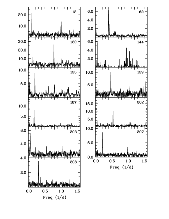
Figure 6: Amplitude spectra of newly detected periodic stars obtained by applying Clean method. Periods corresponding to the detected frequencies for each star are given in Table 1.

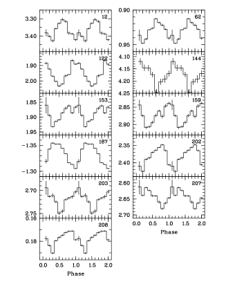
Figure 7: Phased light curves of newly detected periodic stars folded at the detected frequencies. Vertical axis is in magnitude units.

Figure 7 shows phased light curves of the stars shown in Figure 6 at the detected frequencies. Binned phase diagrams are obtained by folding each time series at the detected period. The amplitude of modulation for each star changes between 0.02 and 0.20 magnitude.

We display the power spectra of stars 3 and 20 in Figure 8, together with their phased light curves. Stars 3 and 20 are the samples of stars having shortest and longest periods in our study. The other peaks seen in the top panel are the beat frequencies between the star’s and Earth’s rotation periods. In the middle panel cleaned dirty spectrum obtained by using Clean method is given.

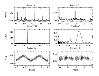
Figure 8: Star 3 and star 20: Stars having the shortest and longest periods in our sample. Upper panel shows the power spectra obtained by Scargle algoritm. Middle panel presents amplitude spectra obtained by Clean algoritm. Lower panel is the phased light curve.

Herbst et al. (2000) indicated that CTTSs were less likely to exhibit periodic variations than WTTSs. Active accretion can prevent any rotational signature. WTTSs are periodic stars. Their cool spots on the surface which are stable for several months (Herbst et al. 2000, Cohen et al. 2004) allow us to detect the rotation period. These cool spots are expected to be associated with magnetic fields. Detection of periodicity could be difficult if the spot pattern and places of them change on a timescale of weeks. The periods determined by Cohen et al. and us are similar, that is they are similar with a maximum change in period by 1$\%$ except for star 114. We observed a period of 15.88 d for this star which is greater about a half day compared to the value of Cohen et al. They detected different periods for this star in different seasons so they gave an average period for five seasons which is 16.40 d. There is a period change of 3$\%$ for this star. This can be related with the chosen Fourier step size which gives a maximum error of 0.7 d. Hence, the stability of rotation periods of TT stars over long time scales is confirmed. Cohen et al. remarks that the longest time that a spot configuration can remain stable enough is between 0.5 and 1 yr.

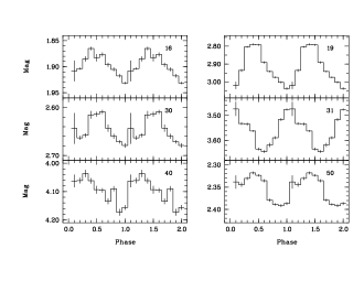
Figure 9: Differential light curves of 6 periodic stars in our sample which were also given by Cohen et al. Numbers for each star refers to HWM catalog.

In Figure 9, we plotted the light curves of 6 periodic stars in our sample which were also plotted by Cohen et al. for the time interval between 1998 and 2003. These plots make stronger the remarks of Cohen et al. about the change of light curve from one season to the other.

The spectral types of stars that we studied are between A0 and M4. For spectral types earlier than late F type Chandra X-ray detection fraction of the cluster is less (Preibisch and Zinnecker 2001). Earlier spectral type stars do not show intrinsic X-ray emission. Therefore, star 94 did not show rotation period. For star 187 which is an A0 type star, we found a period of 6.097 d. Since we do not expect a chromospheric activity that produce X-ray emission from this spectral type, no rotation period should be observed. It can be explained in the way as Preibisch and Zinnecker (2001) explained; that is this rotation period is due to a very close late type companion it is not related with the star itself.

3.2.3 CTT Variables

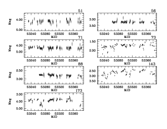
Figure 10: The daily averages of differential light curves of six CTTSs and star 173 which shows large variations in magnitude although classified as WTTS.

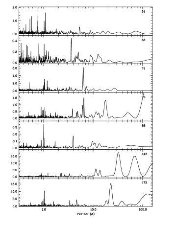
Figure 11: The amplitude spectra for the CTTSs and star 173 of Figure 10.

The daily averages of differential light curves of CTTSs given in Table 1 are plotted in Figure 10. These are stars 51, 56, 71, 73, 88 and 143. The star 73 shows a magnitude variation of 0.7 magnitude. The accretion activity is highly variable in time. The continuous activity of this star with its deep minima is seen clearly from the figure. If we think that minima shows the photospheric luminosities then the increase in luminosity can be caused by the accretion from a disk around the star. Herbig (1998) classifies this star as CTTS (spectral type K0) while Luhmann et al. (1998) measurements of H_α equivalent width indicates a WTTS. H_α emission seems to be time dependent in TT stars (Guenther $\&$ Emmerson 1997). The star 143 also shows similar variations like star 73, showing a magnitude variations of about 1.4 mag. Taking typical mass and radius of a K0 star we can calculate the mass accreted on to the star. If increase in luminosity is arising from the accretion from a disk which is comparable to that of gravitational contraction then a change of 0.7 in magnitude corresponds to a mass accretion rate of Ṁ$\sim 10^{19}$ gr/s. This means that Ṁ is $\sim 10^{-7}$ M_⊙/yr. The other CTTSs are quiet that is variations in their magnitudes are small. The amplitude spectra of these stars are given in Figure 11. Two of them (star 51 and 71) show rotational periodicities whose periods are given in Table 1. Stars 143 and 73 may be in transition phase from CTTS to WTTS as Herbst et al. (2000) and Cohen et al. (2004) suggested. They also suggested that the deep minima seen in the light curves of these stars could be caused by occultation events from dust clouds. The maximum powers calculated are above 5$\sigma$ for these two stars at the detected periods of 6.536 d (for star 73) and 32.28 d (for star 143) which are probably rotation periods. Another star which shows activity in its differential light curve like stars 73 and 143 is star 173 (see Fig.10). This star shows magnitude variations of about 1.5 mag. Herbst et al. classifies this star as an active non periodic WTTS since neither previous study gave the strength of hydrogen emission line (from which Herbst et al. inferred this line was weak). The amplitude spectrum of star 173 (Fig. 11) shows a periodicity at 22.51 d with a 5$\sigma$ confidence level. This star may also be thought as CTTS because of its high activity similar to stars 73 and 143. Star 75 whose rotation period was calculated as 3.088 d was classified as U (unknown class) by Herbst et al. (2000). For this star, Luhman et al. (2003) gives the H_α equivalent width as 10Å. It seems that this star has a phase between CTT and WTT. Nevertheless, its light curve is rather quiet; it does not show any activity in its light curve as in the case of stars 73, 143 and 173.

3.2.4 X-ray Variability and Rotational Periods

In our search we mostly tried to find a period for the optical counterparts of the Chandra sources which are classified as WTTSs. The observed X-ray emission for WTTSs was explained as coronal emission by Preibisch and Zinnecker (2001) and related to the stellar rotation. All WTTSs as possible X-ray sources may not have a variability during the time of observation they may be in their spot less or changing spot pattern period as in the case of stars 77, 103, 115, 148 and 163. To this list we can include also star 17 and 188, since Luhman et al. (2003) gives the H_α equivalent width smaller than 10Å  for these stars. CTTSs have circumstellar accretion disk which could prevent the star to show a regular rotation. CTTSs were also detected as X-ray sources (Preibisch and Zinnecker 2001). Detection frequency among the CTTSs is 45$\%$ while among WTTSs it is 73$\%$. They found no significant difference between the X-ray properties of WTTSs and CTTSs.

Prebisch $\&$ Zinneker (2002) have shown the light curves (count rates) of the sources which shows strong variability during the Chandra observation. For most of these sources we found rotational periods whatever the character of variation of the count rates (flare activity, rising or decaying of count rates).

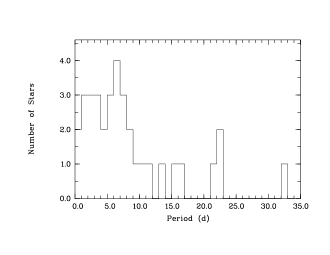
Figure 12: The distribution of rotation periods of sample stars in IC 348 cluster for spectral types earlier than M4

In Figure 12, we plot the distribution of rotation periods in IC 348 cluster using our sample sources for spectral types earlier than M4. The number of stars with slow rotation is less. Cohen et al. (2004) mentioned about the absence of periods shorter than 1 day and deficiency of periods between 4 and 5 days. They said these characteristics were also shared with the period distributions of the Orion Nebula Cluster and Taurus. We have two stars whose periodicity is shorter than 1 day. The plot of IC 348 cluster star distribution is similar to Cohen et al.’s except we have periods shorter than 1 day and longer than 16 days.

Plot of rotational period versus spectral type is shown in Figure 13. There is an increase in period towards the later spectral types. Stars whose spectral types later than K3 have wide range of periods between 0.74 and 32 d. However, an overall gradual increase can not be ruled out. Whereas G and early K dwarfs have smaller rotation periods with a mean value of $\sim 3.7$ days. In Figure 14, we investigate how TTS’s rotation is related to the chromospheric and coronal activity. X-ray luminosities of the sample stars given by Preibisch & Zinnecker (2002) were plotted against the rotational period. Bouvier (1990) proposed that the correlation between X-ray fluxes and rotational periods of TTSs was caused by a solar type dynamo which is responsible for the chromosperic and coronal activity of stars as it is in active dwarfs. Despite the large scatter in the data, there is a trend toward decreasing X-ray luminosity as the rotation period increases. On the other hand stars with periods $<$4 d have an average X-ray luminosity of $\sim 2\times 10^{30}$ erg/sec with a large scatter. As the stars rotate faster their chromospheric and coronal activity increases. Rotation seems to be an important parameter which influences the level of X-ray emission of stars. We note that WTTSs and CTTSs exhibit similar X-ray luminosities at any rotational period. We conclude that X-ray luminosities of TTSs in IC 348 cluster depend on rotation.

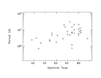
Figure 13: The distribution of rotation periods of sample stars in IC 348 cluster. Open circles denote WTTSs and triangles are CTTSs.

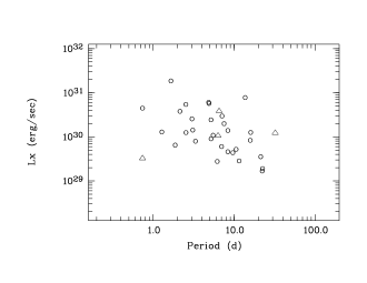
Figure 14: The distribution of X-ray luminosity of sample stars in IC 348 cluster as a function of rotational periods. Open circles denote WTTSs and triangles are CTTSs.

4 Summary

The main results of our analysis of the ROTSE observations of IC 348 cluster can be summarized as follows:

We have 5 months of continuous data of this cluster. In the time series analysis of the stars for the frequency range between 0 and 20 $d^{-1}$ we did not find any periodicity shorter than 0.7 d. Only for the star H254 we confirmed the $\delta$ Scuti pulsation period of 3.24 hr. The other frequencies detected 0.157, 0.283 and 0.931 $d^{-1}$ by Ripepi et al. (2002) for H254 were not present in our light curve.

We found 35 stars as rotationally periodic stars whose rotation periods change between 0.74 and 32.3 d. 18 of them were newly detected periodic stars. 8 of the 18 stars (stars 20, 62, 73, 122, 143, 153, 159, 173) were also studied by Cohen et al. but they did not give any period for these stars. That can be due to the unstable spot patterns during their observation periods. Perhaps the observation duration was not enough to determine the periods. Cohen et al. noted that stars may remain spotted but the spot pattern evolves such that a period can not be determined over 6 consecutive months of observation. Since we detected the periods of these stars it is probably related with the number of data points used in the time series. If the size of the spot is small it can be difficult to detect the period.

Most of the stars whose periods were detected were WTTSs. The periods of non accreting WTTSs are easily detected. There were 7 non periodic WTTSs in our analysis. This may be due to a changing spot pattern or spot less period of the star during the observation. For one of them (star 103) Cohen et al. gives a period of 2.237 d which is an average over all of five seasons they studied. They could not find periodicity for two seasons for this star. The number of CTTSs that we study is less than WTTSs. For the 4 CTTSs (51, 71, 73, 143) we detected rotation period. It would not be possible to detect the periods if the disk prevents the detection of rotational variability. Prebisch $\&$ Zinneker (2002) noted that M type stars without any circumstellar material can show H_α emission. They may not have an accretion disk. H_α emission can also be time dependent in TT stars. These 4 stars may be seen as CTTS at the time of measurement of H_α emission, but at another time H_α emission may be less and they may appear as WTTS.

The rotational periods found in this study are similar with those of Cohen et al. with a maximum change of 1$\%$ in period. Small changes in the rotational periods indicate a rigid rotation. Rotation periods seems to be stable on a timescale of $\sim$6 yr in this cluster when evaluated together with the results of Cohen et al.

We found an inverse correlation between X-ray luminosity and the rotational period in our sample of late type TTSs. X-ray luminosity decreases as the stars rotate slower. WTTSs and CTTSs bahave similar in X-ray activity at any rotational period. The dispersion in rotational periods at a given spectral type results in a dispersion in X-ray luminosity.

Table 1: Properties of Sample IC 348 Field Stars

Star	OTHER IDs	HMW	SP Type	$\sigma_{var}$	Type	Period	Conf
3	LRL22	$\cdots$	G2	0.063	$\cdots$	0.789
8	LRL47	$\cdots$	K0.5	0.039	$\cdots$	4.857
12	LRL87	$\cdots$	M0.7	0.040	(W)	13.73
17	H39	62	M1.5	0.178	U(W)	$\cdots$	$<3\sigma$
20	H43	24	K3.5	0.004	U	21.37
26	H63	52	K8	0.050	W	10.61
32	H70	26	K3	0.008	W	3.021
49	H93	60	M1	0.148	W	7.102
51	H94	59	K7	0.110	C	0.739	$5\sigma$
52	H95	40	K5	0.052	W	8.382	$5\sigma$
56	LRL100	34	M2	0.107	C	$\cdots$	$<3\sigma$
61	H102	39	M1	0.082	W	9.667
62	H103	9	F9Ve	0.023	G	2.548
70	LRL64	19	M0.5	0.052	U(W)	8.385
71	LRL60	133	K8	0.108	C	6.340
73	H114	20	G8	0.249	C	6.536
75	LRL62	31	M4	0.149	U	3.088
77	H116	21	M0	0.035	W	$\cdots$	$<3\sigma$
83	H121	41	K7	0.009	W	7.004
88	H124	75	K6	0.044	C	$\cdots$	$<3\sigma$
94	H252	10	A2	0.004	E	$\cdots$	$<3\sigma$
103	H137	12	K2	0.048	W	$\cdots$	$<3\sigma$
114	H148	44	K7	0.009	W	15.88	$5\sigma$
115	H150	54	M1	0.015	W	$\cdots$	$<3\sigma$
119	H155	50	K5	0.044	W	5.509
122	H157	143	K7	0.024	W	1.280
133	H166	11	G3	0.008	G	1.659	$5\sigma$
137	H171	49	M0	0.042	W	6.207
143	LRL37	23	K6	0.169	C	32.28
144	LRL144	$\cdots$	M0	0.020	(W)	22.31	$5\sigma$
145	H178	16	K6	0.039	W	5.197
146	H179	30	K7	0.108	W	7.532
148	H181	46	M2	0.240	W	$\cdots$	$<3\sigma$
151	H184	14	G7	0.038	G	2.537
153	H187	15	G8	0.063	G	5.203
159	LRl59	18	G7	0.026	G	2.142
163	H198	82	M3	0.142	W	$\cdots$	$<3\sigma$
166	H205	51	M0	0.005	W	11.56
173	H214	56	K8	0.647	W	22.51
176	LRL15	22	M0.5	0.039	C	$\cdots$	$<3\sigma$
187	LRL3	$\cdots$	A0	0.004	$\cdots$	6.097
188	LRL101	$\cdots$	M3.2	0.008	(W)	$\cdots$	$<3\sigma$
202	LRL79	$\cdots$	K0	0.004	$\cdots$	1.872
203	LRL39	$\cdots$	K4	0.048	$\cdots$	16.06
207	LRL1937	$\cdots$	M0	0.043	(W)	4.900
208	LRL20	$\cdots$	G1	0.005	$\cdots$	3.335

Note. — Star numbers are from the catalog (CXOPZ) given by Preibisch & Zinnecker (2001). OTHER IDs starting with H and L are from Herbig (1998) and Luhman et al. (1998) respectively. HMW numbers are from Herbst (2000). Units of $\sigma_{var}$ is magnitude and period is in days.

References

- Akerlof et al. (2003) Akerlof, C. W., Kehoe, R. L., McKay, T. A., Rykoff, E. S., Smith, D. A., et al. 2003, PASP, 115, 132
- Bertin & Arnouts (1996) Bertin, E., & Arnouts, S. 1996, A&AS, 117, 393
- Bouvier (1990) Bouvier, J. 1990, AJ, 99, 946
- Cohen et al. (2004) Cohen, R. E., Herbst, W., & Williams, E. C. 2004, AJ, 127, 1602
- Guenther & Emmerson (1997) Guenther, E. W., & Emmerson, J. P. 1997, A&A, 321, 803
- Harris et al. (1954) Harris D. L., Morgan W. W., Roman N. G., 1954, ApJ, 119, 622
- Herbig (1954) Herbig, G. H. 1954, PASP, 66, 19
- Herbig (1998) Herbig, G. H. 1998, AJ, 497, 736
- Herbst (2000) Herbst, W., Maley, J. A., & Williams, A. J. 2000, AJ, 120, 349
- Lada & Lada (1995) Lada, E. A., & Lada, C. J. 1995, AJ, 109, 1682
- Luhman et al. (1998) Luhman K. L., Rieke, G. H., Lada, C. J., & Lada, E. A. 1998, ApJ, 508, 347
- Luhman et al. (2003) Luhman K. L., Stauffer, J. R., Muench, A. A., Rieke, G. H., Lada, E. A., Bouvier, J., & Lada, C. J. 2003, ApJ, 593, 1093
- Marconi & Palla (1998) Marconi, M., & Palla, F. 1998, ApJ, 507, L141
- Preibisch et al. (1996) Preibisch, Th., Zinnecker, H., & Herbig, G. H. 1996, A&A, 310, 456
- Preibisch & Zinnecker (2001) Preibisch, Th., & Zinnecker, H. 2001, AJ, 122, 866
- Preibisch & Zinnecker (2002) Preibisch, Th., & Zinnecker, H. 2002, AJ, 123, 1613
- Ripepi et al. (2002) Ripepi, V., Palla, F., Marconi, M., Bernabei, S., Arellano Ferro, A., Terranegra, L., & Alcala, J. M. 2002, A&A, 391, 587
- Roberts et al. (1987) Roberts, D. H., Lehar, J., & Dreher, J. W. 1987, AJ, 93, 968
- Scargle (1982) Scargle, J. D. 1982, ApJ, 263, 835
- Trullols & Jordi (1997) Trullols, E., & Jordi, C. 1997, A&A, 324, 549