Abstract

Interferometric observations with three telescopes or more provide two observables: closure phase information together with visibilities measurements. When using single-mode interferometers, both observables have to be redefined in the light of the coupling phenomenon between the incoming wavefront and the fiber. We introduce in this paper the estimator of both so-called modal visibility and modal closure phase. Then, we compute the statistics of the two observables in presence of partial correction by Adaptive Optics, paying attention on the correlation between the measurements. We find that the correlation coefficients are mostly zero and in any case never overtakes $1/2$ for the visibilities, and $1/3$ for the closure phases. From this theoretical analysis, data reduction process using classical least square minimization is investigated. In the framework of the AMBER instrument, the three beams recombiner of the VLTI, we simulate the observation of a single Gaussian source and we study the performances of the interferometer in terms of diameter measurements. We show that the observation is optimized, i.e. that the Signal to Noise Ratio (SNR) of the diameter is maximal, when the full width half maximum (FWHM) of the source is roughly $1/2$ of the mean resolution of the interferometer. We finally point out that in the case of an observation with 3 telescopes, neglecting the correlation between the measurements leads to overestimate the SNR by a factor of $\sqrt{2}$. We infer that in any cases, this value is an upper limit.

OCIS codes: 030.6600, 030.7060, 070.6020, 070.6110, 120.3180

1 Introduction

Thanks to the simultaneous recombination of the light arising from three telescopes, interferometers such as IONIC-3T on IOTA[1] or AMBER on the VLTI[2] are providing closure phase measurements together with the modulus of the visibility. Retrieval of phase information allows to scan the geometry of the source, hence opening the era of image reconstruction with infrared interferometric observations. However, with the current number of telescopes available, direct image restoration requires many successive nights of observations[3]. Thus, in most of the cases where the ($u,v$) coverage spans a relatively small number of spatial frequencies, the measurements have still to be analyzed in the light of model-fitting techniques.

Furthermore, together with partial correction by Adaptive Optics (AO), many of the up-to-date interferometers are making use of waveguides that spatially filters the atmospheric corrugated wavefront, changing the turbulent phase fluctuations into random intensity variations[4] . The estimators that describes the visibility and the closure phase measurements obtained with such interferometers have to account for the coupling between the partially corrected wavefront and the fiber. From these appropriate estimators one can derive the statistical properties of the observables and properly investigate the performances of single-mode interferometers.

In Section 2 we recall the spatial filtering properties of the waveguides in terms of interferometric signal and we define the estimators of both the modal visibility and the closure phase. We investigate in Section 3 the covariance matrices of the observables with respect to atmospheric, photon and detector noises, paying particular attention to the correlation coefficients. Then, defining in Section 4 a general least square model fitting of the measurements, we analyze in Section 5 the ability of fiber optic interferometers to measure stellar diameters.

2 Principles of fiber optic interferometry

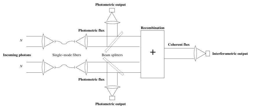
Fig. 1: Sketch of a fiber optic interferometer. Thanks to single mode fibers, beams coming for each telescope are spatially filtered. Then for each beam, a beam splitter is selecting one fraction of the light in order to estimate the photometric flux through dedicated photometric output. The remaining part of the light is recombined with the other beams (recombination is seen here as a black box, and the recombination mode – spatial or temporal – is not a relevant parameter in this study). At the output of the recombination, the coherent flux is estimated thanks to the so-called interferometric output.

A full analysis of the signal arising from fiber optic interferometers has been theoretically described by Mège[5] and summarized by Tatulli et al[6] . We only recall here the important points for this paper, focusing on the coupling phenomenon between the incoming wavefront and the fiber, and on the observables that can be obtained from such interferometers. Figure 1 sketches the principle of a fiber optic interferometer, and reports the main technical terms that will be used all along this paper.

2.A Spatial filtering

Introducing waveguides to carry/recombine the light in an interferometer allows to perform a spatial filtering of the incoming wavefront. It means that the phase corrugation of the wavefront are changed into intensity fluctuations. In other words, the number of photometric and coherent (interferometric) photoevents at the output of the fibers depends on atmospheric fluctuations and results in the coupling between the turbulent wavefront and the fibers[4]^,[7] . Hence, spatial filtering can be seen as coupling coefficients, i.e. the fraction of (respectively photometric and coherent) light that is captured by the fibers. Such coupling coefficients are mathematically described by the following equations[8]^,[9] :

$$\rho_{i}(V_{\star})=\rho_{0}{(V_{\star}*T^{i})_{f=0}}$$ (1)

$$\rho_{ij}(V_{\star})=\rho_{0}(V_{\star}*T^{ij})_{f=f_{ij}}$$ (2)

where $V_{\star}$ is the visibility of the source and $T^{i}$ and $T^{ij}$ are resulting in respectively the auto-correlation and cross-correlation of the aberration-corrupted pupil weighted by the fiber single mode[9]^,[10] :

$$T^{i}(f) = \frac{\int P_{i}(r)P_{i}^{\ast}(r+\lambda{f})\psi_{i}(r)\psi_{i}^{\ast}(r+\lambda{f})\mathrm{d}{r}}{\int|P_{i}(r)|^{2}\mathrm{d}{r}}$$ (3)

$$T^{ij}(f) = \frac{\int P_{i}(r)P_{j}^{\ast}(r+\lambda{f})\psi_{i}(r)\psi_{j}^{\ast}(r+\lambda{f})\mathrm{d}{r}}{\int P_{i}(r)P_{j}^{\ast}(r)\mathrm{d}{r}}$$ (4)

where $P_{i}(r)$ is the pupil function of the $i^{th}$ fiber optic telescope and $\psi_{i}(r)$ is the aberration-corrupted wavefront incoming on the $i^{th}$ pupil. $T^{i}$ and $T^{ij}$ are respectively called the photometric and interferometric peaks. The inverse Fourier transform of $T^{i}$ is called the photometric lobe (or antenna lobe as commonly named in radio) and the inverse Fourier transform of $T^{ij}$ is called the interferometric lobe. $\rho_{0}$ is the optimum coupling efficiency fixed by the fiber core design[11] .

In the case where the source is unresolved by a single telescope (i.e. is much tighter than the photometric lobe), Eq. 1 can be simplified:

$$\rho_{i}(V_{\star})=\rho_{0}\int T^{i}(f)\mathrm{d}{f}=\rho_{0}\mathcal{S}^{i}$$ (5)

where $\mathcal{S}$ is the instantaneous Strehl ratio[12] . Moreover, if the visibility is constant over the range of the high frequency peak $T^{ij}$, the interferometric coupling coefficient has also a simplified expression:

$$|\rho_{ij}(V_{\star})|^{2}=\rho_{0}^{2}\mathcal{S}^{i}\mathcal{S}^{j}|V_{\star}(f_{ij})|^{2}$$ (6)

Under these conditions, the effect of spatial filtering by the fibers in the interferometric equation and, as a result, in the observables, is entirely characterized by the instantaneous Strehl ratio statistics.

2.B Estimation of the modal visibility

We refer to Tatulli et al[6] for a more complete description of the modal visibility. Note however that the expression of the coherent flux at the spatial frequency $f_{ij}$ is given by:

$$I(f_{ij})=\sqrt{K_{i}K_{j}}\rho_{ij}(V_{\star})$$ (7)

where $K_{i}$ and $K_{j}$ are the number of photoevents of telescopes $i$ and $j$ before entering the fiber. An estimator of the modal visibility in the Fourier space is given by the ratio of the coherent flux by the photometric ones, assuming the latter are estimated independently through dedicated photometric outputs (see Fig. 1):

$$\widetilde{V_{ij}^{2}}=\frac{<|I(f_{ij})|^{2}>}{<k_{i}k_{j}>}\left(\frac{\tau}{1-\tau}\right)^{2}$$ (8)

$\tau$ is the fraction of light selected for photometry at the output of the beam-splitter, and $k_{i}$, $k_{j}$ are the photometric fluxes (after the fibers).

2.C Modal bispectrum and closure phase

By definition, the closure phase is the phase of the so called image bispectrum $\widetilde{B}_{klm}$. The latter consists in the ensemble average of the triple product $<\widehat{I}(f_{kl})\widehat{I}(f_{lm})\widehat{I}^{\ast}(f_{km})>$. It can be expressed from Eq. 7 as:

$$\widetilde{B}_{klm}=<K_{k}K_{l}K_{m}\rho_{kl}(V_{\star})\rho_{lm}(V_{\star})\rho^{\ast}_{km}(V_{\star})>$$ (9)

$$=K_{k}K_{l}K_{m}\rho_{0}^{3}\int\!\!\!\!\!\int\!\!\!\!\!\int V_{\star}(f)V_{\star}(f^{{}^{\prime}})V^{\ast}_{\star}(f^{{}^{\prime\prime}}).$$

$$<T^{kl}(f_{kl}-f)T^{lm}(f_{kl}-f^{{}^{\prime}})T^{km^{\ast}}(f_{kl}-f^{{}^{\prime\prime}})>\mathrm{d}{f}\mathrm{d}{f^{{}^{\prime}}}\mathrm{d}{f^{{}^{\prime\prime}}}$$ (10)

Using Roddier’s formalism[13] that demonstrated the bispectrum analysis to be a generalization to the optical of the well known phase closure method currently used in radio interferometry, it is straightforward to notice that the quantity $<T^{kl}(f)T^{lm}(f^{{}^{\prime}})T^{km^{\ast}}(f^{{}^{\prime\prime}})>$ is non zero if $f^{{}^{\prime\prime}}=f+f^{{}^{\prime}}$ and that in this case:

$$<T^{kl}(f)T^{lm}(f^{{}^{\prime}})T^{km^{\ast}}(f^{{}^{\prime\prime}})>=\frac{N(f,f^{{}^{\prime}})}{N^{3}(0)}$$ (11)

$$K_{k}K_{l}K_{m}V_{\star}(f)V_{\star}(f^{{}^{\prime}})V^{\ast}_{\star}(f^{{}^{\prime\prime}})=B_{\star}(f,f^{{}^{\prime}})$$ (12)

where $N(f,f^{{}^{\prime}})$ is proportional to the overlap area of three pupil images shifted apart by the spacings $f$, $f^{{}^{\prime}}$ and $f^{{}^{\prime\prime}}=f+f^{{}^{\prime}}$, and $B_{\star}(f,f^{{}^{\prime}})$ is the bispectrum of the source. Hence the modal bispectrum can be rewritten:

$$\widetilde{B}_{klm}=\rho_{0}^{3}\int\!\!\!\!\!\int B_{\star}(f,f^{{}^{\prime}})\frac{N(f_{kl}-f,f_{lm}-f^{{}^{\prime}})}{N^{3}(0)}\mathrm{d}{f}\mathrm{d}{f^{{}^{\prime}}}$$ (13)

Thus, the modal bispectrum arising from fiber optic interferometers is the source bispectrum integrated over the overlap area $N(f_{kl}-f,f_{lm}-f^{{}^{\prime}})$. Hence, as the modal visibility does not equal in general the object visibility, the modal bispectrum does not coincide with the source bispectrum. Nevertheless, if the source spectrum is constant over the overlap area $N(f_{kl}-f,f_{lm}-f^{{}^{\prime}})$, Eq. 13 takes a simplified form:

$$\widetilde{B}_{klm}=\rho_{0}^{3}B_{\star}(f_{kl},f_{lm})\int\!\!\!\!\!\int\frac{N(f,f^{{}^{\prime}})}{N^{3}(0)}\mathrm{d}{f}\mathrm{d}{f^{{}^{\prime}}}$$ (14)

In this case, the modal bispectrum is proportional to that of the source.

3 The covariance matrices

We propose to characterize the statistics of the square visibility and that of the closure phase (i.e. the bispectrum phase) by computing their respective covariance matrix. Our objective is twofold: derive the error associated to each observable and investigate the degree of dependency of each observable through their correlation coefficients. In order to do so, we use the spatially continuous model of photodetection introduced by Goodman[14]^,[15] where the signal is corrupted by three different types of noise: (i) the signal photon noise; (ii) the additive Gaussian noise of global variance $\sigma^{2}$ which arises from the detector and from thermal emission; (iii) the atmospheric noise resulting from the coupling efficiency variations due to the turbulence. To simplify the calculations, we assume that the source is unresolved by a single aperture, such that the low frequency coupling coefficients verify Eq. 5, and that the source visibility is constant over the range of the interferometric peaks, such that the high frequency coupling coefficients verify Eq. 6. These assumptions drive to neglect the modal speckle noise regime – it has been shown that the modal speckle noise is rejected towards negative magnitudes and only affects very bright sources[6] – and to only focus on “photon noise” and “detector noise” regimes . The full calculations of the covariance coefficients of the visibilities and of the closure phases are done in Appendix A. They lead to relatively complicated formulae which depend on the Strehl statistics. Using a simple analytical approach, we derive in Appendix Bthe mean and the variance of the Strehl as a function of the turbulence strength and the level of AO correction. The relative error of the Strehl is bounded between two limit values[10]^,[14] :

$$\mathrm{(Perfect~{}correction)}~{}~{}0\leq\frac{\sigma_{\mathcal{S}}}{\overline{\mathcal{S}}}\leq 1~{}~{}\mathrm{(No~{}correction)}$$ (15)

Table 1. gives the expressions of the limiting values of the variance of the visibility and the closure phase for a point source in both “photon noise” and “detector noise” regimes. The error of the visibility will be deeply used in the next section to derive the performances of the Very Large Telescope Interferometer (VLTI) with regards to single sources diameter measurements. Let us concentrate in this part on the correlation coefficients of the visibilities and the closure phases, respectively. Their limiting values are summarized in Table 2. Clearly, for visibilities the correlation coefficients are null in the photon noise regime when no telescope is in common (see Fig. 2.) and are always smaller than $1/2$ otherwise, and for the closure phases they are null when no baseline is in common (see Fig. 3.) and are always smaller than $1/3$ otherwise. Furthermore, the relative number of null elements in the covariance matrices rapidly increases with the number of telescopes. It implies that if there are $(N-1)(N-2)/2$ linearly independent closure phase relations[16] , the whole set of $N(N-1)(N-2)/6$ closure phase relations can be considered in first approximation as statistically independent.

It would be of great interest to pursue this study by comparing the statistics of the closure phase to that of the phase measured by phase referencing technique. The formalism presented in Appendix A can indeed be transposed to the phase referencing case, but it requires a dedicated analysis which is beyond the scope of the present paper.

4 Model fitting

The present generation of interferometers only provides small number of telescopes (basically $2$ or $3$). In such a case, it is frequent that the lack of spatial frequencies in the $(u,v)$ coverage prevents from image reconstruction of the studied object. Hence, the measurements have to be analyzed in the light of a model of the object. We propose here a simple $\chi^{2}$ model-fitting of the observables.

Let us define $\widehat{O}_{\theta}$ as the normalized spectrum of the object model characterized by a set of parameters $\theta$. From this spectrum we derive the model of the observables that have to be fitted according to the measurements:

Square visibility	$\displaystyle|\widehat{O}_{\theta}|^{2}(f_{ij})$
Closure Phase	$\displaystyle\phi_{G}=\arctan\left[\frac{\mathrm{Im}(G_{\theta})}{\mathrm{Re}(G_{\theta})}\right]$

where $G_{\theta}^{klm}=\widehat{O}_{\theta}(f_{kl})\widehat{O}_{\theta}(f_{lm})\widehat{O}_{\theta}^{\ast}(f_{km})$ is the bispectrum model. Then, the estimated parameters $\widetilde{\theta}$ constraining at best the observations are obtained by minimizing the distance between the model and the measurements. Assuming Gaussian statistics for the observables, the distance is given by the well known $\chi^{2}$:

$$\chi^{2}_{tot}=\chi^{2}_{V^{2}}+\chi^{2}_{\phi_{B}}$$ (16)

with

$$\chi^{2}_{V^{2}}=\left[\widetilde{V^{2}}-|\widehat{O}_{\theta}|^{2}\right]C_{V^{2}}^{-1}\left[\widetilde{V^{2}}-|\widehat{O}_{\theta}|^{2}\right]^{T}$$ (17)

$$\chi^{2}_{\phi_{B}}=\left[\widetilde{\phi}_{B}-\phi_{G}\right]C_{\phi_{B}}^{-1}\left[\widetilde{\phi}_{B}-\phi_{G}\right]^{T}$$ (18)

where $X^{T}$ denotes the transpose of the vector $X$. Equation 16 supposes that the two observables of different nature (i.e. the visibility and the closure phase) are uncorrelated. Such assumption seems quite reasonable since we have shown that two measurements of same nature are already poorly correlated.

It can be argued that, in order to avoid phase discontinuities issues, it might be better to work on the phasor (i.e. the average bispectrum) than on the phase of the average bispectrum. In that case the $\chi^{2}$ constraint takes the form:

$$\chi^{2}_{B}=\left[\mathrm{Im}\left(\widetilde{B}G_{\theta}^{\ast}\right)\right]C_{\mathrm{Im}\left(\widetilde{B}G_{\theta}^{\ast}\right)}^{-1}\left[\mathrm{Im}\left(\widetilde{B}G_{\theta}^{\ast}\right)\right]^{T}$$ (19)

Such constraint does not appear to be appropriate for two reasons: (i) constraining the average bispectrum or the closure phase of the average bispectrum is strictly equivalent when the latter shows good SNR; (ii) the covariance depends on the model which makes the $\chi^{2}$ minimization subject to biases due to improper noise estimates. For very noisy data, the closure phase shows a lot of discontinuities and its probability law, wrapped around $[-\pi,\pi]$, tends towards a uniform law. Such a case, for which the $\chi^{2}$ fitting method is no more optimal, neither for the closure phase nor for the bispectrum, corresponds in practice to the sensitivity limit of the instrument.

Putting Equation 16 into the generic form:

$$\chi^{2}(\theta)=\mathcal{M}_{\theta}\mathcal{C}_{\mathcal{M}}^{-1}\mathcal{M}_{\theta}^{T}$$ (20)

the error of the estimated parameters $\widetilde{\theta}$ writes[17] :

$$\sigma^{2}(\widetilde{\theta})=\mathrm{Diag}\left\{\left[\mathcal{A}^{T}\mathcal{C}_{\mathcal{M}}^{-1}\mathcal{A}\right]^{-1}\right\}$$ (21)

where

$$\mathcal{A}=\frac{\partial\mathcal{M}_{\theta}}{\partial\theta}\bigg{|}_{\theta=\widetilde{\theta}}$$ (22)

5 Applications

5.A Observing a single Gaussian source

We propose in this section to simulate the observation of a single Gaussian source of FWHM $\sigma_{O}$, with AMBER, the three beam recombiner of the VLTI[2] . Since the object is centro-symmetrical, closure phase is not relevant and hence all the information is contained in the visibility alone. For sake of simplicity, we first neglect the contribution of the correlation coefficients. Their effect will be studied in Section 5.C. We adopt the standard instrumental configuration of AMBER[18] in which the signal is sampled over $N_{pix}=16$ pixels. We choose a spectral resolution of $35$ in the $K$ band ($2.2\mu m$), an integration time of $30\mathrm{ms}$ per interferogram, a transmission coefficient $\tau=0.5$, a readout noise of $15\mathrm{e}^{-}/\mathrm{pix}$ and an optimized coupling coefficient of $\rho_{0}=0.8$[11] . We observe an object with $2$ Unit Telescopes (UT2 and UT4, $D=8\mathrm{m}$) during $4\mathrm{H}$ (half of the time on the object, half of the time on the calibrator) with $5\mathrm{min}$ per frequency point which, together with the integration time per interferogram, leads to $5000$ samples per frequency point. Note that all along the observation, the length of the projected baseline is quite constant with $B=45\mathrm{m}\pm 2\mathrm{m}$. Finally, we assume a turbulence strength of $D/r_{0}=5$ and a typical AO correction of $\mathcal{S}=0.5$.

Fig. 4. shows the SNR of the object size as the function of the magnitude. We consider different sizes: $\sigma_{o}=1\mathrm{mas}$, $\sigma_{o}=3.8\mathrm{mas}$, $\sigma_{o}=5.4\mathrm{mas}$, and $\sigma_{o}=10.8\mathrm{mas}$, which are to be compared to $\lambda/B\sim 10\mathrm{mas}$, the resolution of the interferometer. As expected, a general profile can be seen with two well known regimes: the “photon noise” regime for bright sources and the “detector noise” regime for faint sources. Defining the limiting magnitude as the magnitude for which the SNR is equal to $1$, we find $\mathcal{K}\sim 11-13$ according to the size of the source.

Clearly, the SNR first increases and then decreases with the size of the source, reaching a maximum around $\sigma_{o}=4\mathrm{mas}$. This phenomenon can be understood as follows: for marginally resolved sources, the parameters of the fit are barely constrained and the SNR is small. It increases with the size up to a point where the available projected baseline range does not match anymore the frequency content of the object. From there, the SNR begins to drop. This trend stands for all observing conditions, but as we show in the next section the exact position of the maximum depends on the noise regime.

5.B Optimizing the baseline

We simulate different configurations with two telescopes that span the range of average projected baseline, respectively: (a) $B=45\mathrm{m}$ ($+$); (b) $B=56\mathrm{m}$ ($\times$); (c) $B=83\mathrm{m}$ ($\diamond$); (d) $B=100\mathrm{m}$ ($\triangle$); (e) $B=124\mathrm{m}$ ($\square$). The declination of the source is arbitrarily set to $-25^{\circ}$. The source is supposed to be observed between $-3\mathrm{h}$ to $3\mathrm{h}$ from the zenith. The parameters of the different configurations used are summarized in Table 3 and corresponding $(u,v)$ plane coverages are shown in Fig. 5. (up).

We compute the SNR of the diameter for all these configurations, in both “detector noise” ($K=13$) and “photon noise” ($K=2$) regimes, respectively. In the “detector noise” regime, the error of the visibility is independent on the diameter, and since in this case Eq. 21 tells us that $\sigma(\widetilde{\theta})$ is directly inversely proportional to $\displaystyle\frac{\partial\mathcal{M}_{\theta}}{\partial\theta}\bigg{|}_{\theta=\widetilde{\theta}}$, the SNR of the diameter is maximum when the product of the diameter by the derivative of the model is maximum too, namely when:

$$\frac{\partial}{\partial\theta}\left[\theta\frac{\partial\mathcal{M}_{\theta}}{\partial\theta}\right]\Bigg{|}_{\theta=\widetilde{\theta}}=\frac{\partial}{\partial\theta}\left[\theta\frac{\partial|\widehat{O}_{\theta}|^{2}}{\partial\theta}\right]\Bigg{|}_{\theta=\widetilde{\theta}}=0$$ (23)

This leads to:

$$\widetilde{\sigma}_{o}=\frac{2\sqrt{ln(2)}}{\pi\sqrt{2}}\frac{\lambda}{<B>}\simeq 0.38\frac{\lambda}{<B>}$$ (24)

where $<B>$ is th average projected baseline.

In the “photon noise” regime, the error of the visibility is strongly dependent on the size. In that case, the maximum of the SNR occurs when the projected baseline range scanned by the interferometer matches the object frequency content. Considering the frequency for which the visibility is $1/\mathrm{e}$, it comes:

$$\widetilde{\sigma}_{o}=\frac{2\sqrt{ln(2)}}{\pi}\frac{\lambda}{<B>}\simeq 0.54\frac{\lambda}{<B>}$$ (25)

Fig. 5. (middle and bottom) illustrates these results. The SNR of the diameter is plotted as a function of the size in $\lambda/B$ units, for the five geometrical configurations selected above. We can see that the whole curves present the same behavior, and especially the same maximum. This maximum verifies Eq.’s 24 and 25 for the “detector noise” and the “photon noise” regimes, respectively. We conclude that the mean projected baseline optimizing the observation of an object of diameter $\sigma_{o}$ is given by:

$$<B>\simeq 0.5\frac{\lambda}{\sigma_{o}}$$ (26)

Furthermore we stress that the performances degrades rapidly when this criterion is not respected.

5.C Effect of the correlation coefficients on the error bars

We have shown in Section 3 that the correlations between the visibilities could reach a maximum value of $\rho=0.5$. Since the estimator arising from maximum likelihood (i.e. the $\chi^{2}$ minimization) is unbiased, the expected value of the fitted parameters does not depend on whether the correlation coefficients are introduced or not. We analyze here the effect of the correlation coefficients on the derived error.

We simulate the observation of a Gaussian source with three UTs, together with the instrumental parameters of Section 5 and we choose $\sigma_{o}=0.5\lambda/<B>$ for the FWHM of the source. Fig. 6. shows, in both pure turbulent ($\sigma_{\mathcal{S}}=\overline{\mathcal{S}}$) and fully AO corrected ($\sigma_{\mathcal{S}}=0$) cases, the SNR of $\sigma_{o}$, with and without taking into account the correlation coefficients. It results that considering uncorrelated measurements leads to underestimate the error (or overestimate the SNR) by a factor of $\sqrt{2}$, roughly. Given that the ratio of the null elements versus the non null elements in the covariance matrix increases with the number of telescopes, we infer that this factor $\sqrt{2}$ is an upper limit.

6 Summary

We have computed the theoretical covariance matrices of the modal visibility and the modal closure phase in the presence of partial AO correction, when the measurements are corrupted by atmospheric, photon and detector noises. In the photon noise regime and for an interferometer with a large number of telescopes, the measurements are most of the time uncorrelated. In any case, the correlation coefficients are always smaller than $1/2$ for the visibilities and smaller than $1/3$ for the closure phases.

Then from a classical least square approach, we have investigated the ability of interferometers to measure stellar diameters. In the light of the AMBER experiment we have found a limiting magnitude in the range $K=11-13$ depending on the size of the source. At last, we have shown that the observation is optimized when the mean resolution of the interferometer is equal to twice the stellar diameter.

APPENDIX A: STATISTICS OF THE OBSERVABLES

1. General formalism

In order to compute the moments of the spectral density, we use the spatially continuous model of photodetection process of Goodman[14] where the detected signal is corrupted by photon noise, by additive Gaussian noise $\epsilon$ of variance $\sigma^{2}$ and by the turbulent atmosphere. It takes the form:

$$s(x,y)=\sum_{n=1}^{K}\delta(x-x_{n})+\epsilon(x)$$ (A-1)

and its Fourier transform:

$$\widehat{S}(f)=\sum_{n=1}^{K}\exp\left(-2i\pi{fx_{n}}\right)+\widehat{\epsilon}(f)$$ (A-2)

2. The modal visibility

Such calculation has been already done in Tatulli et al[6] . We give here the results assuming that the low and high coupling coefficients verify Eq. 5 and 6 respectively. We remind that following equations assume also that the telescope transmissions are all equal, i.e. $K_{i}=K/N_{tel}$, where $K_{i}$ is the number of photoevents coming from telescope $i$ and $N_{tel}$ is the number of the telescope, and that the level of corrections of the Adaptive Optics systems are the same for all the telescopes.

The square relative error of the modal visibility can be seen as the sum of two contributions:

$$\frac{\sigma^{2}\{V_{ij}^{2}\}}{\overline{V_{ij}^{2}}^{2}}=\mathcal{E}^{2}_{P}(K,\mathcal{S})+\mathcal{E}^{2}_{A}(K,\sigma^{2},\mathcal{S})$$ (A-3)

with $\mathcal{E}^{2}_{P}$ the photon noise square relative error and $\mathcal{E}^{2}_{A}$ the additive noise relative error, as described in Tatulli et al[6] . The same way, the covariance can be cut in two terms:

$$\frac{\mathrm{Cov}\left\{V_{ij}^{2},V_{kl}^{2}\right\}}{\overline{V_{ij}^{2}}\overline{V_{kl}^{2}}}=\mathcal{C}_{P}(K,\mathcal{S})+\mathcal{C}_{A}(K,\sigma^{2},\mathcal{S})$$ (A-4)

Here we must pay attention that two cases can occur (see Fig. 2. in the body of the text): (i) either the baselines $f_{ij}$ and $f_{kl}$ come from two distinct pairs of telescopes (ii) either the baselines have one telescope in common, let say $j=k$, which drives to extra correlation between the visibilities.

The results, i.e. the diagonal and non diagonal terms of the visibility covariance matrix, are summarized in table 4.

3. The closure phase

The estimator of the bispectrum between telescopes $i,j,k$ is defined by:

$$Q_{ijk}=\widehat{S}(f_{ij})\widehat{S}(f_{jk})\widehat{S}^{\ast}(f_{ik})$$ (A-5)

Chelli[15] has shown that the covariance (per sample) on the closure phase does only depend on the modulus of the bispectrum, and hence assuming a centro-symmetrical source, could be written:

$$\mathrm{Cov}\left\{\Phi_{ijk},\Phi_{lmn}\right\}=\frac{1}{2}\frac{\mathrm{Re}[Q_{ijk}(Q_{lmn}-Q^{\ast}_{lmn})]}{\mathrm{E}(Q_{ijk})\mathrm{E}(Q_{lmn})}$$ (A-6)

with

$$\mathrm{E}(Q_{ijk}) = <\overline{K}^{3}\widehat{i}(f_{ij})\widehat{i}(f_{jk})\widehat{i}^{\ast}(f_{kl})>_{\phi}$$ (A-7)

$$= \overline{\mathcal{S}}^{3}[V_{\star}(f_{ij})V_{\star}(f_{jk})V_{\star}^{\ast}(f_{ik})]\frac{\rho_{0}^{3}\overline{K}^{3}}{N_{tel}^{3}}$$ (A-8)

where $\widehat{i}(f)$ is the normalized spectral density.

For sake of simplicity we analyze the second order moments of the estimator in two cases separately: the “photon noise” case and the “detector noise” case. Then the statistics with regards to the atmosphere are taken into account.

4. The photon noise case

Following Goodman’s formalism[14]^,[15] the second order moments are:

$$\mathrm{E}_{K}\{|Q_{ijk}|^{2}\} = \overline{K}^{3}+\overline{K}^{4}\left[|\widehat{i}(f_{ij})|^{2}+|\widehat{i}(f_{jk})|^{2}+|\widehat{i}(f_{ik})|^{2}\right]$$ (A-9)

$$+\overline{K}^{5}\left[|\widehat{i}(f_{ij})|^{2}|\widehat{i}(f_{jk})|^{2}+|\widehat{i}(f_{ij})|^{2}|\widehat{i}(f_{ik})|^{2}+|\widehat{i}(f_{jk})|^{2}|\widehat{i}(f_{ik})|^{2}\right]$$

$$+\overline{K}^{6}\left[|\widehat{i}(f_{ij})|^{2}|\widehat{i}(f_{jk})|^{2}|\widehat{i}(f_{ik})|^{2}\right]$$

$$\mathrm{E}_{K}\{Q_{12}^{2}\} = 2\overline{K}^{3}\left[\widehat{i}^{\ast}(f_{ij})\widehat{i}^{\ast}(f_{jk})\widehat{i}(f_{ik})\right]+\overline{K}^{4}\left[|\widehat{i}(f_{ij})|^{4}+|\widehat{i}(f_{jk})|^{4}+|\widehat{i}(f_{ik})|^{4}\right.$$ (A-10)

$$+\left.2|\widehat{i}(f_{ij})|^{2}|\widehat{i}(f_{jk})|^{2}+2|\widehat{i}(f_{ij})|^{2}|\widehat{i}(f_{ik})|^{2}+2|\widehat{i}(f_{jk})|^{2}|\widehat{i}(f_{ik})|^{2}\right]$$

$$+2\overline{K}^{5}\left[\widehat{i}(f_{ij})\widehat{i}(f_{jk})\widehat{i}^{\ast}(f_{ik})|\widehat{i}(f_{ij})|^{2}+|\widehat{i}(f_{jk})|^{2}+|\widehat{i}(f_{ik})|^{2})\right]$$

$$+\overline{K}^{6}\left[\widehat{i}(f_{ij})\widehat{i}(f_{jk})\widehat{i}^{\ast}(f_{ik})\right]^{2}$$

For the covariance, two cases may appear (see Fig. 3. in the body of the text): (i) both triplets of telescopes ($i,j,k$ and $l,m,n$) are different or (ii) two telescopes are part of both triplets, in that case there is a baseline in common, let say $f_{ij}=f_{lm}$. This add extra terms in the covariance.

$$\mathrm{E}_{K}\{Q_{ijk}Q_{lmn}^{\ast}\} = \overline{K}^{6}\left[\widehat{i}(f_{ij})\widehat{i}(f_{jk})\widehat{i}^{\ast}(f_{ik})\widehat{i}^{\ast}(f_{lm})\widehat{i}^{\ast}(f_{mn})\widehat{i}(f_{ln})\right]$$ (A-11)

$${\mathrm{if}~{}~{}f_{ij}=f_{lm}}$$

$$+\overline{K}^{3}|\widehat{i}(f_{kn})|^{2}+\overline{K}^{4}|\widehat{i}(f_{ij})|^{2}|\widehat{i}(f_{kn})|^{2}$$

$$+\overline{K}^{4}\left[\widehat{i}(f_{kn})\widehat{i}(f_{ik})\widehat{i}^{\ast}(f_{ln})+\widehat{i}(f_{kn})\widehat{i}(f_{jk})\widehat{i}^{\ast}(f_{mn})\right]$$

$$+\overline{K}^{5}\left[\widehat{i}(f_{jk})\widehat{i}^{\ast}(f_{ik})\widehat{i}^{\ast}(f_{mn})\widehat{i}(f_{ln})\right]$$

$$+\overline{K}^{5}|\widehat{i}(f_{ij})|^{2}\left[\widehat{i}(f_{kn})\widehat{i}(f_{ik})\widehat{i}^{\ast}(f_{ln})+\widehat{i}(f_{kn})\widehat{i}(f_{jk})\widehat{i}^{\ast}(f_{mn})\right]$$

$$\mathrm{E}_{K}\{Q_{ijk}Q_{lmn}\} = \overline{K}^{6}\left[\widehat{i}(f_{ij})\widehat{i}(f_{jk})\widehat{i}^{\ast}(f_{ik})\widehat{i}(f_{lm})\widehat{i}(f_{mn})\widehat{i}^{\ast}(f_{ln})\right]$$ (A-12)

$${\mathrm{if}~{}~{}f_{ij}=f_{lm}}$$

$$+\overline{K}^{4}\left[|\widehat{i}(f_{mn})|^{2}|\widehat{i}(f_{ik})|^{2}+|\widehat{i}(f_{mn})|^{2}|\widehat{i}(f_{jk})|^{2}\right]$$

$$+\overline{K}^{4}\left[|\widehat{i}(f_{ln})|^{2}|\widehat{i}(f_{ik})|^{2}+|\widehat{i}(f_{ln})|^{2}|\widehat{i}(f_{jk})|^{2}\right]$$

$$+\overline{K}^{5}\left[\widehat{i}(f_{jk})\widehat{i}^{\ast}(f_{ik})\widehat{i}^{\ast}(f_{mn})\widehat{i}(f_{ln})\right]$$

$$+\overline{K}^{5}\left[\widehat{i}(f_{ij})\widehat{i}(f_{jk})\widehat{i}^{\ast}(f_{ik})(|\widehat{i}(f_{mn})|^{2}+|\widehat{i}(f_{ln})|^{2})\right]$$

$$+\overline{K}^{5}\left[\widehat{i}(f_{lm})\widehat{i}(f_{mn})\widehat{i}^{\ast}(f_{ln})(|\widehat{i}(f_{jk})|^{2}+|\widehat{i}(f_{ik})|^{2})\right]$$

5. The detector noise case

We suppose a zero mean Gaussian detector noise of variance $\sigma^{2}$.

$$\mathrm{E}_{\epsilon}\{|Q_{ijk}|^{2}\} = \overline{K}^{6}\left[|\widehat{i}(f_{ij})|^{2}|\widehat{i}(f_{jk})|^{2}|\widehat{i}(f_{ik})|^{2}\right]$$ (A-13)

$$+N\sigma^{2}\overline{K}^{4}\left[|\widehat{i}(f_{ij})|^{2}|\widehat{i}(f_{jk})|^{2}+|\widehat{i}(f_{ij})|^{2}|\widehat{i}(f_{ik})|^{2}+|\widehat{i}(f_{jk})|^{2}|\widehat{i}(f_{ik})|^{2}\right]$$

$$+(3N\sigma^{4}+N^{2}\sigma^{4})\overline{K}^{2}\left[|\widehat{i}(f_{ij})|^{2}|\widehat{i}(f_{jk})|^{2}|\widehat{i}(f_{ik})|^{2}\right]$$

$$+N^{3}\sigma^{6}+3N^{2}\sigma^{6}+15N\sigma^{6}$$

$$\mathrm{E}_{\epsilon}\{Q_{ijk}^{2}\} = \overline{K}^{6}\left[\widehat{i}(f_{ij})\widehat{i}(f_{jk})\widehat{i}^{\ast}(f_{ik})\right]^{2}+15N\sigma^{6}$$ (A-14)

$$\mathrm{E}_{\epsilon}\{Q_{ijk}Q_{lmn}^{\ast}\} = \overline{K}^{6}\left[\widehat{i}(f_{ij})\widehat{i}(f_{jk})\widehat{i}^{\ast}(f_{ik})\widehat{i}^{\ast}(f_{lm})\widehat{i}^{\ast}(f_{mn})\widehat{i}(f_{ln})\right]+15N\sigma^{6}$$ (A-15)

$${\mathrm{if}~{}~{}f_{ij}=f_{lm}}$$

$$+N\sigma^{2}\overline{K}^{4}\left[\widehat{i}(f_{ij})\widehat{i}^{\ast}(f_{ik})\widehat{i}^{\ast}(f_{mn})\widehat{i}(f_{ln})\right]+3N^{2}\sigma^{6}$$

$$\mathrm{E}_{\epsilon}\{Q_{ijk}Q_{lmn}\} = \overline{K}^{6}\left[\widehat{i}(f_{ij})\widehat{i}(f_{jk})\widehat{i}^{\ast}(f_{ik})\widehat{i}(f_{lm})\widehat{i}(f_{mn})\widehat{i}^{\ast}(f_{ln})\right]+15N\sigma^{6}$$ (A-16)

Once taking into account the statistics with regards to the atmospheric turbulence, the final expression are given in both “photon noise” and “detector noise” regime in tables 5 and 6, respectively.

The expression of the covariance in the general case is obtained by adding the covariance in each regime:

$$\mathrm{Cov}\left\{\Phi_{ijk},\Phi_{lmn}\right\}=\mathrm{Cov}_{phot}\left\{\Phi_{ijk},\Phi_{lmn}\right\}+\mathrm{Cov}_{det}\left\{\Phi_{ijk},\Phi_{lmn}\right\}$$ (A-17)

APPENDIX B: MODELLING PARTIAL ADAPTIVE OPTICS CORRECTION

We consider a simplified model where the long exposure AO corrected transfer function can be divided in two weighted components: one perfect transfer function and one turbulent transfer function where the weight $h$ describes the strength of the correction:

$$<T^{i}(f)> = \frac{T^{i}_{0}(f)}{\int T^{i}_{0}(f)\mathrm{d}{f}}[h+(1-h)\mathcal{B}_{\phi}(f)],~{}h\in[0,1]$$ (B-1)

$$= \frac{T^{i}_{0}(f)}{\int T^{i}_{0}(f)\mathrm{d}{f}}\exp\left[-\frac{1}{2}\mathcal{D}_{\phi}(f)\right]$$

where $\mathcal{D}_{\phi}(f)$ is the AO corrected structure function. For sake of simplicity we assume that the transfer function of the turbulence $\mathcal{B}_{\phi}(f)$ is Gaussian, hence:

$$\mathcal{B}_{\Phi}=\exp\left(-\frac{f^{2}}{\sigma_{\mathcal{B}}^{2}}\right),\sigma_{\mathcal{B}}=\sqrt{\frac{2}{6.88}}\frac{r_{0}}{\lambda}$$ (B-2)

Going further we can notice that the AO corrected transfer function of the atmosphere can be decomposed in a low frequency term (halo) and a high frequency term (coherent energy)[19] :

$$\exp\left[-\frac{1}{2}\mathcal{D}_{\phi}(f)\right]=\mathrm{FTO}_{halo}+\exp(-\sigma^{2}_{\phi})$$ (B-3)

and that,

$$\exp\left[-\frac{1}{2}\mathcal{D}_{\phi}(f)\right]=h+(1-h)\mathcal{B}_{\phi}(f)$$ (B-4)

Hence we have:

$$h=\exp(-\sigma^{2}_{\phi})=\mathrm{E}_{c}(D/r_{0},N_{z})$$ (B-5)

where the coherent energy $\mathrm{E}_{c}$ depends on the level of correction (number of Zernike $N_{z}$) and the strength of the turbulence $D/r_{0}$.

Using the definition of the long exposure Strehl ratio:

$$\overline{\mathcal{S}}=\int<T^{i}(f)>\mathrm{d}{f}$$ (B-6)

it comes:

$$\overline{\mathcal{S}}=h+(1-h)\frac{\sigma^{2}_{\mathcal{B}}}{\sigma^{2}_{\mathcal{B}}+\sigma^{2}_{T}}=\mathrm{E}_{c}+\frac{(1-\mathrm{E}_{c})}{1+3.44\left(\frac{D}{r_{0}}\right)^{2}}$$ (B-7)

The second order moment of the instantaneous Strehl ratio writes:

$$\overline{\mathcal{S}^{2}} = \iint<T^{i}(f)T^{i}(f^{{}^{\prime}})>\mathrm{d}{f}\mathrm{d}{f^{{}^{\prime}}}$$ (B-8)

$$= \iint P_{i}(r)P_{i}(r+\rho)P_{i}(r^{{}^{\prime}})P_{i}(r^{{}^{\prime}}+\rho^{{}^{\prime}})$$

$$\times<\Psi_{i}(r)\Psi_{i}^{\ast}(r+\rho)\Psi_{i}^{\ast}(r^{{}^{\prime}})\Psi_{i}(r^{{}^{\prime}}+\rho^{{}^{\prime}})>\mathrm{d}{r}\mathrm{d}{\rho}\mathrm{d}{r^{{}^{\prime}}}\mathrm{d}{\rho^{{}^{\prime}}}$$

where $P_{i}(r)$ is the pupil function and $\Psi_{i}(r)$ is the complex amplitude of the AO corrected wavefront. We use Korff’s[20] derivation of the moments of the complex amplitude of the wavefronts to introduce in the equations linear combinations of the structure function ($\mathcal{D}(r)$) at different spatial frequencies. Assuming the structure function to be stationary, it comes:

$$\overline{\mathcal{S}^{2}} = P_{i}(r)P_{i}(r+\rho)P_{i}(r^{{}^{\prime}})P_{i}(r^{{}^{\prime}}+\rho^{{}^{\prime}}).$$ (B-9)

$$\frac{\exp\left\{-\frac{1}{2}[\mathcal{D}(\rho)+\mathcal{D}(\rho^{{}^{\prime}})+\mathcal{D}(r^{{}^{\prime}}-r)+\mathcal{D}(r^{{}^{\prime}}+\rho^{{}^{\prime}}-r-\rho)]\right\}}{\exp\left\{-\frac{1}{2}[\mathcal{D}(r^{{}^{\prime}}+\rho^{{}^{\prime}}-r)+\mathcal{D}(r^{{}^{\prime}}-r-\rho)]\right\}}\mathrm{d}{r}\mathrm{d}{\rho}\mathrm{d}{r^{{}^{\prime}}}\mathrm{d}{\rho^{{}^{\prime}}}$$

Using Eq. B-4, previous expression can be analytically developed for $h=\mathrm{E_{c}}=]0.5,1]$, i.e. for good AO correction levels[6] . However we know that, without AO correction and assuming circular Gaussian statistics for the complex amplitude of the wavefront, we have $\sigma_{\mathcal{S}}=\overline{\mathcal{S}}$[10]^,[14] . Hence we can perform an interpolation between the good AO corrections and the pure turbulent cases. Fig 7. shows the SNR of the Strehl ratio as a function respectively of the number of Zernike (i.e. the correction level) and the average Strehl ratio $\overline{\mathcal{S}}$, at different $D/r_{0}$. For each curve, we point out where from the interpolation has been done.

Table 1: Variance of the visibility and the closure phase for a point source. $N_{pix}$ corresponds to the number of pixels that sample the interferogram. $N_{pix}\geq 2$ is required to respect the Shannon criterion. $\sigma$ is the detector noise per pixel.

	Variance of the observables (point source)
Observables	Photon noise regime ($\overline{K}\gg 1$)
			Detector noise regime
			($\overline{K}\ll 1$)
	Full AO correction	No AO correction
$\ \widetilde{V^{2}}$	$\left[\frac{2N_{tel}}{(1-\tau)}+\frac{2}{\tau}\right]\frac{N_{tel}}{\rho_{0}\overline{\mathcal{S}}\overline{K}}$	$\left[\frac{2N_{tel}+4}{(1-\tau)}+\frac{4}{\tau}\right]\frac{N_{tel}}{\rho_{0}\overline{\mathcal{S}}\overline{K}}$	$\left[\frac{3N_{pix}\sigma^{4}+N_{pix}^{2}\sigma^{4}}{(1-\tau)^{4}}\right]\frac{N_{tel}^{4}}{\rho_{0}^{4}\overline{\mathcal{S}}^{4}\overline{K}^{4}}$
$\widetilde{\phi}_{B}$	$\left[\frac{3N_{tel}-6}{2}\right]\frac{N_{tel}}{\rho_{0}\overline{\mathcal{S}}\overline{K}}$	$\left[\frac{3N_{tel}-3}{2}\right]\frac{N_{tel}}{\rho_{0}\overline{\mathcal{S}}\overline{K}}$	$\left[\frac{9N_{pix}\sigma^{4}+3N_{pix}^{2}\sigma^{4}}{2}\right]\frac{N_{tel}^{4}}{\rho_{0}^{4}\overline{\mathcal{S}}^{4}\overline{K}^{4}}$

Table 2: Correlation coefficients of the visibilities and the closure phases. For the visibility, two cases are considered: one telescope is common to both baselines, hence the triplet of telescopes is forming a triangle (a so-called closure), or not (see Fig. 2.). For the closure phases, two cases are investigated as well: one baseline belongs to both closure phases or not (see Fig. 3).

		Correlation coefficient $\rho$ (point source)
Observables		Photon noise regime ($\overline{K}\gg 1$)
				Detector noise regime
				($\overline{K}\ll 1$)
		Full AO correction	No AO correction
	if closure	$\displaystyle\leqslant\frac{1}{2}$	$\displaystyle\leqslant\frac{1}{4}$
$\displaystyle\widetilde{V^{2}}$				$\displaystyle\frac{3}{3+N_{pix}}$
	otherwise	$\displaystyle 0$	$\displaystyle 0$
	if baseline in common	$\displaystyle\frac{1}{3}$	$\displaystyle\leqslant\frac{1}{6}$	$\displaystyle\frac{3}{9+N_{pix}}$
$\displaystyle\widetilde{\phi}_{B}$
	otherwise	$\displaystyle 0$	$\displaystyle 0$	$\displaystyle 0$

Table 3: Description of the considered telescopes configurations. Are given the name of the telescopes pairs, their respective average projected baseline as well as the related symbols used in Fig. 5. The telescopes are the four $8$ meters Unit telescopes (UTs) of the VLTI. The declination of the source is arbitrarily set to $-25^{\circ}$. The source is supposed to be observed between $-3\mathrm{h}$ to $3\mathrm{h}$ from the zenith.

Symbol	Telescopes	Average projected baseline
$+$	UT2-UT3	$45\mathrm{m}$
$\times$	UT1-UT2	$56\mathrm{m}$
$\diamond$	UT2-UT4	$83\mathrm{m}$
$\triangle$	UT1-UT3	$100\mathrm{m}$
$\square$	UT1-UT4	$124\mathrm{m}$

Table 4: Description of the elements of the visibility covariance matrix.

Observables	Covariance coefficients
	Diagonal	$\displaystyle\left[\frac{4\sigma^{2}_{\mathcal{S}}+2N_{tel}\overline{\mathcal{S}}^{2}}{(1-\tau)V_{\star}^{2}(f_{ij})\overline{\mathcal{S}}^{3}}+\frac{2(\sigma^{2}_{\mathcal{S}}+\overline{\mathcal{S}}^{2})}{\tau\overline{\mathcal{S}}^{3}}\right]\frac{N_{tel}}{\rho_{0}\overline{K}}+\left[\frac{2N_{tel}\sigma^{2}_{\mathcal{S}}+N_{tel}^{2}\overline{\mathcal{S}}^{2}}{(1-\tau)^{2}V_{\star}^{4}(f_{ij})\overline{\mathcal{S}}^{4}}+\frac{4}{(1-\tau)^{2}V_{\star}^{2}(f_{ij})\overline{\mathcal{S}}^{2}}+\frac{1}{\tau^{2}\overline{\mathcal{S}}^{2}}\right]\frac{N_{tel}^{2}}{{\rho_{0}^{2}\overline{K}^{2}}}+\frac{1}{(1-\tau)^{3}V_{\star}^{4}(f_{ij})\overline{\mathcal{S}}^{3}}\frac{N_{tel}^{4}}{{\rho_{0}^{3}\overline{K}^{3}}}$
Visibility	coefficients	$\displaystyle+\left[\frac{2N\sigma^{2}}{(1-\tau)^{2}V_{\star}^{2}(f_{ij})\overline{\mathcal{S}}^{2}}\right]\frac{N_{tel}^{2}}{\rho_{0}^{2}\overline{K}^{2}}+\left[\frac{2N\sigma^{2}}{(1-\tau)^{3}V_{\star}^{4}(f_{ij})\overline{\mathcal{S}}^{3}}\right]\frac{N_{tel}^{4}}{\rho_{0}^{3}\overline{K}^{3}}+\left[\frac{3N\sigma^{4}+N^{2}\sigma^{4}}{(1-\tau)^{4}V_{\star}^{4}(f_{ij})\overline{\mathcal{S}}^{4}}\right]\frac{N_{tel}^{4}}{\rho_{0}^{4}\overline{K}^{4}}$
$\displaystyle\frac{\mathrm{Cov}\left\{V_{ij}^{2},V_{kl}^{2}\right\}}{\overline{V_{ij}^{2}}\overline{V_{kl}^{2}}}$	Non diagonal	$\displaystyle\left[\frac{2}{(1-\tau)^{2}\overline{\mathcal{S}}^{2}}\left[\frac{1}{V_{\star}^{2}(f_{ij})}+\frac{1}{V_{\star}^{2}(f_{kl})}\right]+\frac{N_{tel}\sigma^{2}_{\mathcal{S}}}{(1-\tau)^{2}V_{\star}^{2}(f_{ij})V_{\star}^{2}(f_{kl})\overline{\mathcal{S}}^{4}}\right]\frac{N_{tel}^{2}}{\rho_{0}^{2}\overline{K}^{2}}+\left[\frac{1}{(1-\tau)^{3}V_{\star}^{2}(f_{ij})V_{\star}^{2}(f_{kl})\overline{\mathcal{S}}^{3}}\right]\frac{N_{tel}^{4}}{\rho_{0}^{3}\overline{K}^{3}}+\left[\frac{3N\sigma^{4}}{(1-\tau)^{4}V_{\star}^{2}(f_{ij})V_{\star}^{2}(f_{kl})\mathcal{S}^{4}}\right]\frac{N_{tel}^{4}}{\rho_{0}^{4}\overline{K}^{4}}$
	coefficients	$\displaystyle{\mathrm{if}~{}~{}j=k}+\frac{1}{\tau\overline{\mathcal{S}}}\frac{N_{tel}}{\rho_{0}\overline{K}}+\left[\frac{2\mathrm{Re}[V_{\star}(f_{ij})V_{\star}(f_{kl})V^{\ast}_{\star}(f_{il})]}{(1-\tau)V_{\star}^{2}(f_{ij})V_{\star}^{2}(f_{kl})\overline{\mathcal{S}}}\right]\frac{N_{tel}}{\rho_{0}\overline{K}}+\left[\frac{V_{\star}^{2}(f_{il})}{(1-\tau)^{2}V_{\star}^{2}(f_{ij})V_{\star}^{2}(f_{kl})\mathcal{S}^{2}}\right]\frac{N_{tel}^{2}}{\rho_{0}^{2}\overline{K}^{2}}$

Table 5: Description of the elements of the closure phase covariance matrix, in the “photon noise” regime.

Observables	Covariance coefficients
		$\displaystyle\left[\frac{[N_{tel}^{3}-2V_{\star}^{\ast}(f_{ij})V_{\star}^{\ast}(f_{jk})V_{\star}(f_{ik})]\overline{\mathcal{S}}^{3}+3N_{tel}^{2}\sigma^{2}_{\mathcal{S}}\overline{\mathcal{S}}}{2|V_{\star}(f_{ij})|^{2}|V_{\star}(f_{jk})|^{2}|V_{\star}(f_{ik})|^{2}\overline{\mathcal{S}}^{6}}\right]\frac{N_{tel}^{3}}{\rho_{0}^{3}\overline{K}^{3}}+\left[\frac{[|V_{\star}(f_{ij})|^{2}+|V_{\star}(f_{jk})|^{2}+|V_{\star}(f_{ik})|^{2}][N_{tel}^{2}\overline{\mathcal{S}}^{4}+N_{tel}\sigma^{2}_{\mathcal{S}}\overline{\mathcal{S}}^{2}+2\sigma^{4}_{\mathcal{S}}]}{2|V_{\star}(f_{ij})|^{2}|V_{\star}(f_{jk})|^{2}|V_{\star}(f_{ik})|^{2}\overline{\mathcal{S}}^{6}}\right]\frac{N_{tel}^{2}}{\rho_{0}^{2}\overline{K}^{2}}$
	Diagonal	$\displaystyle-\left[\frac{[|V_{\star}(f_{ij})|^{4}+|V_{\star}(f_{jk})|^{4}+|V_{\star}(f_{ik})|^{4}][\overline{\mathcal{S}}^{4}+2\sigma^{2}_{\mathcal{S}}\overline{\mathcal{S}}^{2}+\sigma^{4}_{\mathcal{S}}]+2[|V_{\star}(f_{ij})|^{2}|V_{\star}(f_{jk})|^{2}+|V_{\star}(f_{ik})|^{2}(|V_{\star}(f_{jk})|^{2}+|V_{\star}(f_{ij})|^{2})][\overline{\mathcal{S}}^{4}+\sigma^{2}_{\mathcal{S}}\overline{\mathcal{S}}^{2}]}{2|V_{\star}(f_{ij})|^{2}|V_{\star}(f_{jk})|^{2}|V_{\star}(f_{ik})|^{2}\overline{\mathcal{S}}^{6}}\right]\frac{N_{tel}^{2}}{\rho_{0}^{2}\overline{K}^{2}}$
	coefficients	$\displaystyle+\left[\frac{[|V_{\star}(f_{ij})|^{2}|V_{\star}(f_{jk})|^{2}+|V_{\star}(f_{ik})|^{2}(|V_{\star}(f_{jk})|^{2}+|V_{\star}(f_{ij})|^{2})][N_{tel}\overline{\mathcal{S}}^{5}+(N_{tel}+4)\sigma^{2}_{\mathcal{S}}\overline{\mathcal{S}}^{3}+2\sigma^{4}_{\mathcal{S}}\overline{\mathcal{S}}]}{2|V_{\star}(f_{ij})|^{2}|V_{\star}(f_{jk})|^{2}|V_{\star}(f_{ik})|^{2}\overline{\mathcal{S}}^{6}}\right]\frac{N_{tel}}{\rho_{0}\overline{K}}$
Closure phase		$\displaystyle-\left[\frac{2[V_{\star}(f_{ij})V_{\star}(f_{jk})V_{\star}^{\ast}(f_{ik})][|V_{\star}(f_{ij})|^{2}+|V_{\star}(f_{jk})|^{2}+|V_{\star}(f_{ik})|^{2}][\overline{\mathcal{S}}^{5}+2\sigma^{2}_{\mathcal{S}}\overline{\mathcal{S}}^{3}+\sigma^{4}_{\mathcal{S}}\mathcal{S}]}{2|V_{\star}(f_{ij})|^{2}|V_{\star}(f_{jk})|^{2}|V_{\star}(f_{ik})|^{2}\overline{\mathcal{S}}^{6}}\right]\frac{N_{tel}}{\rho_{0}\overline{K}}$
		$0~{}~{}~{}$ if $f_{ij}\neq f_{lm}$
$\displaystyle\mathrm{Cov}\left\{\Phi_{ijk},\Phi_{lmn}\right\}$
		$\displaystyle\left[\frac{|V_{\star}(f_{kn})|^{2}[N_{tel}\overline{\mathcal{S}}^{3}+2\sigma^{2}_{\mathcal{S}}\overline{\mathcal{S}}]}{2V_{\star}(f_{ij})V_{\star}(f_{jk})|V_{\star}^{\ast}(f_{ik})V^{\ast}_{\star}(f_{lm})V^{\ast}_{\star}(f_{mn})|V_{\star}(f_{ln})\overline{\mathcal{S}}^{6}}\right]\frac{N_{tel}^{3}}{\rho_{0}^{3}\overline{K}^{3}}$
	Non diagonal	$\displaystyle+\left[\frac{[|V_{\star}(f_{ij})|^{2}|V_{\star}(f_{kn})|^{2}]\overline{\mathcal{S}}^{4}+[V_{\star}(f_{kn})V_{\star}^{\ast}(f_{mn})V_{\star}^{\ast}(f_{mk})+V_{\star}(f_{kn})V_{\star}^{\ast}(f_{lk})V_{\star}^{\ast}(f_{ln})][N_{tel}\overline{\mathcal{S}}^{4}+3\sigma^{2}_{\mathcal{S}}\overline{\mathcal{S}}^{2}]}{2V_{\star}(f_{ij})V_{\star}(f_{jk})|V_{\star}^{\ast}(f_{ik})V^{\ast}_{\star}(f_{lm})V^{\ast}_{\star}(f_{mn})|V_{\star}(f_{ln})\overline{\mathcal{S}}^{6}}\right]\frac{N_{tel}^{2}}{\rho_{0}^{2}\overline{K}^{2}}$
	coefficients	$\displaystyle-\left[\frac{[|V_{\star}(f_{ik})|^{2}|V_{\star}(f_{in})|^{2}+|V_{\star}(f_{jk})|^{2}|V_{\star}(f_{jn})|^{2}][\overline{\mathcal{S}}^{4}+\sigma^{2}_{\mathcal{S}}\overline{\mathcal{S}}^{2}]+[|V_{\star}(f_{ik})|^{2}|V_{\star}(f_{jn})|^{2}+|V_{\star}(f_{in})|^{2}|V_{\star}(f_{jk})|^{2}]}{2V_{\star}(f_{ij})V_{\star}(f_{jk})|V_{\star}^{\ast}(f_{ik})V^{\ast}_{\star}(f_{lm})V^{\ast}_{\star}(f_{mn})|V_{\star}(f_{ln})\overline{\mathcal{S}}^{6}}\right]\overline{\mathcal{S}}^{4}\frac{N_{tel}^{2}}{\rho_{0}^{2}\overline{K}^{2}}$
		$\displaystyle\left[\frac{[V_{\star}(f_{jk})V_{\star}^{\ast}(f_{ik})V_{\star}^{\ast}(f_{jn})V_{\star}(f_{in})][N_{tel}\overline{\mathcal{S}}^{5}+4\sigma^{2}_{\mathcal{S}}\overline{\mathcal{S}}^{3}]+[V_{\star}(f_{kn})V_{\star}^{\ast}(f_{in})V_{\star}^{\ast}(f_{ik})+V_{\star}(f_{kn})V_{\star}(f_{jk})V_{\star}^{\ast}(f_{jn})]|V_{\star}(f_{ij})|^{2}[\overline{\mathcal{S}}^{5}+\sigma^{2}_{\mathcal{S}}\overline{\mathcal{S}}^{3}]}{2V_{\star}(f_{ij})V_{\star}(f_{jk})|V_{\star}^{\ast}(f_{ik})V^{\ast}_{\star}(f_{lm})V^{\ast}_{\star}(f_{mn})|V_{\star}(f_{ln})\overline{\mathcal{S}}^{6}}\right]\frac{N_{tel}}{\rho_{0}\overline{K}}$
		$\displaystyle-\left[\frac{[V_{\star}(f_{ij})V_{\star}(f_{jk})V_{\star}^{\ast}(f_{ik})(|V_{\star}(f_{in})|^{2}+|V_{\star}(f_{jn})|^{2})+V_{\star}(f_{ij})V_{\star}(f_{jn})V_{\star}^{\ast}(f_{in})(|V_{\star}(f_{jk})|^{2}+|V_{\star}(f_{ik})|^{2})][\overline{\mathcal{S}}^{5}+\sigma^{2}_{\mathcal{S}}\overline{\mathcal{S}}^{3}]}{2V_{\star}(f_{ij})V_{\star}(f_{jk})|V_{\star}^{\ast}(f_{ik})V^{\ast}_{\star}(f_{lm})V^{\ast}_{\star}(f_{mn})|V_{\star}(f_{ln})\overline{\mathcal{S}}^{6}}\right]\frac{N_{tel}}{\rho_{0}\overline{K}}~{}~{}~{}$ if $f_{ij}=f_{lm}$

Table 6: Description of the elements of the closure phase covariance matrix, in the “detector noise” regime.

Observables	Covariance coefficients
	Diagonal	$\displaystyle\left[\frac{[|V_{\star}(f_{ij})|^{2}+|V_{\star}(f_{jk})|^{2}+|V_{\star}(f_{ik})|^{2}][3N\sigma^{4}+N^{2}\sigma^{4}]\overline{\mathcal{S}}^{2}}{2|V_{\star}(f_{ij})|^{2}|V_{\star}(f_{jk})|^{2}|V_{\star}(f_{ik})|^{2}\overline{\mathcal{S}}^{6}}\right]\frac{N_{tel}^{4}}{\rho_{0}^{4}\overline{K}^{4}}$
Closure phase	coefficients	$\displaystyle+\left[\frac{[|V_{\star}(f_{ij})|^{2}|V_{\star}(f_{ij})|^{2}+|V_{\star}(f_{jk})|^{2}|V_{\star}(f_{jk})|^{2}+|V_{\star}(f_{ik})|^{2}|V_{\star}(f_{ij})|^{2}]N\sigma^{2}[\overline{\mathcal{S}}^{4}+\sigma^{2}_{\mathcal{S}}\overline{\mathcal{S}}^{2}]}{2|V_{\star}(f_{ij})|^{2}|V_{\star}(f_{jk})|^{2}|V_{\star}(f_{ik})|^{2}\overline{\mathcal{S}}^{6}}\right]\frac{N_{tel}^{2}}{\rho_{0}^{2}\overline{K}^{2}}+N^{3}\sigma^{6}+3N^{2}\sigma^{6}$
		$0~{}~{}~{}$ if $f_{ij}\neq f_{lm}$
$\displaystyle\mathrm{Cov}\left\{\Phi_{ijk},\Phi_{lmn}\right\}$	Non diagonal
	coefficients	$\displaystyle\left[\frac{[V_{\star}(f_{jk})V_{\star}^{\ast}(f_{ik})V_{\star}^{\ast}(f_{jn})V_{\star}(f_{in})]N\sigma^{2}\overline{\mathcal{S}}^{4}}{2V_{\star}(f_{ij})V_{\star}(f_{jk})|V_{\star}^{\ast}(f_{ik})V^{\ast}_{\star}(f_{lm})V^{\ast}_{\star}(f_{mn})|V_{\star}(f_{ln})\overline{\mathcal{S}}^{6}}\right]\frac{N_{tel}^{2}}{\rho_{0}^{2}\overline{K}^{2}}+3N^{2}\sigma^{6}~{}~{}~{}$ if $f_{ij}=f_{lm}$

Fig. 2: This figure shows the configurations that have to be considered when computing the covariance of the visibilities. Respectively no telescope in common (left) or one telescope in common, hence forming a closure (right).

Fig. 3: This figure shows configurations that have to be considered when computing the covariance of the closure phases. Respectively no baseline (left) or one baseline (right) in common between both triplets of telescopes.

Fig. 4: SNR of the diameter $\sigma_{o}$ as a function of the magnitude. Different sizes are considered: $\sigma_{o}=1\mathrm{mas}$ (dash-dotted line) , $\sigma_{o}=3.8\mathrm{mas}$ (dotted line), $\sigma_{o}=5.4\mathrm{mas}$ (solid line), $\sigma_{o}=10.8\mathrm{mas}$ (dashed line). The resolution is $\lambda/B=10\mathrm{mas}$. $\mathcal{S}=0.5$, $D/r_{0}=5$.

Fig. 5: Up: $(u,v)$ coverage for different UTs configurations. The average projected baseline length is respectively: $B=45\mathrm{m}$ ($+$), $B=56\mathrm{m}$ ($\times$), $B=83\mathrm{m}$ ($\diamond$), $B=100\mathrm{m}$ ($\triangle$), $B=124\mathrm{m}$ ($\square$). More informations about the different configurations considered are given in Table 3. Middle: SNR of the diameter as a function of the size given in fraction of the interferometer resolution $\lambda/B$, in the “detector noise” regime. Vertical line shows the size where the SNR is maximum. Bottom: same as above, but in the “photon noise” regime.

Fig. 6: SNR of the diameter as a function of the magnitude, for perfect AO correction (upper curves, $\sigma_{\mathcal{S}}=0$) and in the pure turbulent case (lower curves, $\sigma_{\mathcal{S}}=\overline{\mathcal{S}}$). SNR is computed assuming diagonal covariance of the measurements (no correlation: solid line) or considering correlation coefficients as computed in Section 3 (dashed lines).

Fig. 7: SNR of the Strehl ratio as a function of the level of correction in number of corrected Zernike (top), and as a function of the long exposure Strehl ratio (bottom). Results are given for $D/r_{0}=1$ (solid line), $D/r_{0}=2$ (dashed line), $D/r_{0}=5$ (dash-dotted line), $D/r_{0}=10$ (dotted line). Vertical lines show from where the interpolation has been performed.

References

• [1] J.ย Berger, P.ย Haguenauer, P.ย Y. Kern, K.ย Rousselet-Perraut, F.ย Malbet, S.ย Gluck, L.ย Lagny, I.ย Schanen-Duport, E.ย Laurent, A.ย Delboulbe, E.ย Tatulli, W.ย A. Traub, N.ย Carleton, R.ย Millan-Gabet, J.ย D. Monnier, E.ย Pedretti, and S.ย Ragland, โ€œAn integrated-optics 3-way beam combiner for IOTA,โ€ in Interferometry for Optical Astronomy II. Edited by Wesley A. Traub . Proceedings of the SPIE, Volume 4838, pp. 1099-1106 (2003)., pp. 1099โ€“1106 (2003).
• [2] R.ย G. Petrov, F.ย Malbet, A.ย Richichi, K.ย Hofmann, D.ย Mourard, K.ย Agabi, P.ย Antonelli, E.ย Aristidi, C.ย Baffa, U.ย Beckmann, P.ย Berio, Y.ย Bresson, and F.ย Cassaing, โ€œAMBER: the near-infrared focal instrument for the Very Large Telescope Interferometer,โ€ in Proc. SPIE Vol. 4006, p. 68-79, Interferometry in Optical Astronomy, Pierre J. Lena; Andreas Quirrenbach; Eds., pp. 68โ€“79 (2000).
• [3] E.ย Thiรฉbaut, P.ย J.ย V. Garcia, and R.ย Foy, โ€œImaging with Amber/VLTI: the case of microjets,โ€ Astrophysics and Space Science 286, 171โ€“176 (2003).
• [4] V.ย Coudรฉ du Foresto, Fringe benefits: the spatial filtering advantages of single-mode fibers, pp. 27โ€“30 (Integrated Optics for Astronomical Interferometry, Grenoble, 1997).
• [5] P.ย Mรจge, โ€œInterfรฉromรฉtrie avec des guides dโ€™onde optiques: thรฉorie et applicationsโ€, Ph.D.ย Thesis, Universitรฉ Joseph Fourier, Grenoble (2002).
• [6] E.ย Tatulli, P.ย Mรจge, and A.ย Chelli, โ€œSingle-mode versus multimode interferometry: A performance study,โ€ Astronomy and Astrophysics 418, 1179โ€“1186 (2004).
• [7] C.ย Ruilier, โ€œA study of degraded light coupling into single-mode fibers,โ€ in Proc. SPIE Vol. 3350, p. 319-329, Astronomical Interferometry, Robert D. Reasenberg; Ed., pp. 319โ€“329 (1998).
• [8] S.ย D. Dyer and D.ย A. Christensen, โ€œPupil-size effects in fiber optic stellar interferometry,โ€ Optical Society of America Journal 16, 2275โ€“2280 (1999).
• [9] P.ย Mรจge, F.ย Malbet, and A.ย Chelli, โ€œStellar Interferometry with optical waveguides,โ€ in SF2A-2001: Semaine de lโ€™Astrophysique Francaise, Lyon, May 28-June 1st 2001, pp. 581โ€“+ (2001).
• [10] F.ย Roddier, โ€œOptical Propagation and Image Formation Through the Turbulent Atmosphere,โ€ in Diffraction-Limited Imaging with Very Large Telescopes Cargese, September 13-23 1988, pp. 33โ€“+ (1989).
• [11] S.ย Shaklan and F.ย Roddier, โ€œCoupling starlight into single-mode fiber optics,โ€ Appl.ย  Opt.ย 27, 2334โ€“2338 (1988).
• [12] V.ย Coudรฉ du Foresto, M.ย Faucherre, N.ย Hubin, and P.ย Gitton, โ€œUsing single-mode fibers to monitor fast Strehl ratio fluctuations. Application to a 3.6 m telescope corrected by adaptive optics,โ€ Astronomy and Astrophysics Supplement 145, 305โ€“310 (2000).
• [13] F.ย Roddier, โ€œTriple correlation as a phase closure technique,โ€ Optics Communications 60, 145โ€“148 (1986).
• [14] J.ย W. Goodman, โ€œStatistical Optics,โ€ Optical Society of America Journal 2, 1455โ€“+ (1985).
• [15] A.ย Chelli, โ€œThe phase problem in optical interferometry - Error analysis in the presence of photon noise,โ€ Astronomy and Astrophysics 225, 277โ€“290 (1989).
• [16] J.ย D. Monnier, โ€œAn Introduction to Closure Phases,โ€ in Principles of Long Baseline Stellar Interferometry, Michelson Summer School, August 15-19, 1999, pp. 203โ€“+ (2000).
• [17] K.ย von der Heide and G.ย Knoechel, โ€œStatistically rigorous reduction of stellar polarization measurements,โ€ Astronomy and Astrophysics 79, 22โ€“26 (1979).
• [18] F.ย Malbet, A.ย Chelli, and R.ย G. Petrov, โ€œAMBER performances: signal-to-noise ratio analysis,โ€ in Proc. SPIE Vol. 4006, p. 233-242, Interferometry in Optical Astronomy, Pierre J. Lena; Andreas Quirrenbach; Eds., pp. 233โ€“242 (2000).
• [19] J.-M. Conan, โ€œร‰tude de la correction partielle en optique adaptativeโ€, Ph.D.ย Thesis, Universitรฉ Paris XI Orsay (1994).
• [20] D.ย Korff, โ€œAnalysis of a Method for Obtaining Near Diffraction Limited Information in the Presence of Atmospheric Turbulence,โ€ Optical Society of America Journal 63, 971โ€“980 (1973).