Simple Models for the Distribution of Dark Matter

We introduce a simple family of models for representing the dark matter in galaxies. The potential and phase space distribution function are all elementary, while the density is cusped. The models are all hypervirial, that is, the virial theorem holds locally, as well as globally. As an application to dark matter studies, we compute some of the properties of $\gamma$-ray sources caused by neutralino self-annihilation in dark matter clumps.

1 Introduction

It is worthwhile to find simple models for the distribution of dark matter in galaxy haloes. This is tantamount to solving the collisionless Boltzmann and Poisson equations for the distribution function (DF) $f$, potential $\psi$, and density $\rho$ of the dark matter particles.

Many authors start by assuming a profile for the dark matter density and then solving for the self-consistent potential and DF. This has provided some widely-used and notable models for dark matter haloes (e.g., Jaffe 1983; Hernquist 1990). A drawback to this approach is that, even if the density and potential are simple, the DF is often unwieldy. For example, the DF of the Jaffe (1983) model is a higher transcendental function, while the DF of the Hernquist (1990) model is composed of an unwieldy bunch of elementary functions.

It can be advantageous to tackle this problem the other way around, by assuming a simple DF and then solving for the self-consistent potential and the density. Except for Toomre (1982), this reverse approach has not been widely used. Here, we exploit it to build a flexible family of cusped dark matter halo models with an elementary DF and potential (Sects. 2 & 3).

As a simple application, we use our models to study the signal from indirect detection experiments (Sect. 4). In particular, $\gamma$-rays from dark matter annihilation may be identified by forthcoming atmospheric Čerenkov telescopes such as VERITAS or by satellite-borne detectors like GLAST, and so it is useful to have definite predictions from halo models.

2 A Simple distribution function

2.1 An ansatz

Let us assume that the dark halo is spherical, in which case the DF may depend on the binding energy $E$ and the magnitude of the angular momentum $L$. Let us note that the generalized Plummer models, recently studied by Evans & An (2005) have very simple power-law DFs of the form

$$f(E,L)\propto L^{p-2}E^{(3p+1)/2}.$$ (1)

This suggests that it may be worthwhile to look for models with DFs given by the sum of such components (c.f., Fricke 1952; Toomre 1982);

$$f(E,L)=\sum_{i}C_{i}L^{p_{i}-2}E^{(3p_{i}+1)/2}.$$ (2)

where $C_{i}$ and $p_{i}$ are all constants. Then, the density is of the form

$$\rho=\sum_{i}D_{i}r^{p_{i}-2}\psi^{2p_{i}+1},$$ (3)

where the constants $D_{i}$ are

$$D_{i}=2^{(p_{i}+1)/2}\piup^{3/2}C_{i}\frac{\Gamma(p_{i}/2)\Gamma(3p_{i}/2+3/2)}{\Gamma(2p_{i}+2)}.$$ (4)

By integrating the DF over velocity space, it is straightforward to derive the radial and tangential velocity second moments $\langle v_{r}^{2}\rangle$ and $\langle v_{\mathrm{T}}^{2}\rangle$ respectively. Whereas the anisotropy parameter $\beta=1-\langle v_{\mathrm{T}}^{2}\rangle/(2\langle v_{r}^{2}\rangle)$ is no longer constant in contrast to models of Evans & An (2005), we still find the remarkably simple relation between the three-dimensional velocity dispersion and the potential;

$$\langle v_{r}^{2}\rangle+\langle v_{\mathrm{T}}^{2}\rangle=\frac{\psi}{2}.$$ (5)

In other words, the root mean square velocity is always one-half of the escape velocity at every spot, or the virial theorem holds locally for any model described by the DF of Eq. (2). Evans & An (2005) coined the term “hypervirial” to describe such stellar dynamical models for which the kinetic energy in each volume element ($T=\rho\langle v^{2}\rangle/2$) is exactly one-half of the magnitude of the local contribution to the potential energy by the same volume element ($|W|=\rho\psi/2$). This idea can be traced back to the classical investigations of Plummer (1911) and Eddington (1916). It has received additional impetus from the recent $N$-body simulations of Sota et al. (2005).

2.2 Poisson’s equation

While we have established that any spherical system described by a DF of the form of Eq. (2) is hypervirial, we still have to find the corresponding density and potential by solving Poisson’s equation (here $G=1$)

$$\frac{1}{r^{2}}\frac{\mathrm{d}}{\mathrm{d}r}\left(r^{2}\frac{\mathrm{d}\psi}{\mathrm{d}r}\right)=-4\piup\sum_{i}D_{i}r^{p_{i}-2}\psi^{2p_{i}+1}.$$ (6)

The order of Eq. (6) can be reduced as follows (c.f., Chandrasekhar 1939). First, let us consider the substitution $\psi=r^{-1/2}\varphi=\varphi\exp(-t/2)$ and $t=\ln r$. Then, the left hand side of Eq. (6) transforms

$$\frac{1}{r^{2}}\frac{\mathrm{d}}{\mathrm{d}r}\left(r^{2}\frac{\mathrm{d}\psi}{\mathrm{d}r}\right)=r^{-5/2}\left(\frac{\mathrm{d}^{2}\varphi}{\mathrm{d}t^{2}}-\frac{\varphi}{4}\right),$$ (7)

while the right hand side can be rewritten using

$$\sum_{i}D_{i}r^{p_{i}-2}\psi^{2p_{i}+1}=\sum_{i}D_{i}r^{-5/2}\varphi^{2p_{i}+1}.$$ (8)

Hence, Eq. (6) reduces to

$$\frac{\mathrm{d}^{2}\varphi}{\mathrm{d}t^{2}}=\frac{\varphi}{4}-4\piup\sum_{i}D_{i}\varphi^{2p_{i}+1},$$ (9)

which does not involve the independent variable explicitly, and so its order can be reduced by standard techniques (e.g., Ince 1944) to give

$$\left(\frac{\mathrm{d}\varphi}{\mathrm{d}t}\right)^{2}=A+\frac{\varphi^{2}}{4}\left(1-\sum_{i}4B_{i}\varphi^{2p_{i}}\right),$$ (10)

where $A$ is a constant of integration and

$$B_{i}=\frac{4\piup D_{i}}{p_{i}+1}.$$ (11)

Using the boundary condition at infinity ($\varphi=0$ and $\mathrm{d}\varphi/\mathrm{d}t=0$), we find that $A=0$. Then, after introducing a further transformation of the variable, $\varphi^{-p}=\vartheta$, Eq. (10) reduces to

$$\left(-\frac{2}{p}\frac{\mathrm{d}\vartheta}{\mathrm{d}t}\right)^{2}=\vartheta^{2}-\sum_{i}4B_{i}\vartheta^{2(1-p_{i}/p)}.$$ (12)

Here, we note that the differential equation $(y^{\prime})^{2}=f(y)$ where $f(y)$ is a polynomial of $y$, the degree of which is at most two, can be solved through elementary functions. However, the right-hand side of Eq. (12) can be a quadratic polynomial of $\vartheta$ if $p=p_{i}$ or $p=2p_{i}$ for all distinct $p_{i}$’s. For the simplest case when the sum contains only a single term, it is straightforward to show that either choice of $p$ leads to the solution that reduces to the models of Evans & An (2005) with the integration constant being the scalelength. The only other possibility is that the sum contains two terms with $p=p_{1}=2p_{2}$, which is investigated in the following section.

2.3 Solutions

For this case, the integration results in

$$\vartheta=2k\cosh\left[\frac{p}{2}(t\!-\!t_{0})\right]+2B_{2}=k\left[\left(\frac{r}{r_{0}}\right)^{p/2}\!\!+\left(\frac{r}{r_{0}}\right)^{-p/2}\right]+2B_{2},$$ (13)

where $t_{0}=\ln r_{0}$ is the integration constant, and $k=(B_{1}+B_{2}^{2})^{1/2}$. By reinstating $\vartheta=\varphi^{-p}=r^{-p/2}\psi^{-p}$, we obtain

$$\frac{1}{\psi^{p}}=kr_{0}^{p/2}\left[1+2c\left(\frac{r}{r_{0}}\right)^{p/2}\!\!+\left(\frac{r}{r_{0}}\right)^{p}\right],$$ (14)

where $c=B_{2}/k$. With the normalization $M_{\infty}=1$, we find that $k=r_{0}^{p/2}$. So, we arrive at a two-parameter – $c$ and $p$ – potential of the form of (incorporating the dimensional constants $G$, $M$ and $r_{0}$)

$$\psi=\frac{GM}{\left(r_{0}^{p}+2cr_{0}^{p/2}r^{p/2}+r^{p}\right)^{1/p}},$$ (15)

whose DF is given by

$$f(E,L)=C_{1}L^{p-2}E^{3p/2+1/2}+C_{2}L^{p/2-2}E^{3p/4+1/2}.$$ (16)

Here, the constants $C_{i}$ can be found from Eqs. (4) and (11) with $B_{1}=1-c^{2}$, $B_{2}=c$, $p_{1}=p$ and $p_{2}=p/2$ (henceforth $G=M=r_{0}=1$), that is,

$$C_{1} = \frac{1-c^{2}}{2^{p/2+1}(2\piup)^{5/2}}\frac{\Gamma(2p+3)}{\Gamma(p/2)\Gamma(3p/2+3/2)}$$

$$C_{2} = \frac{c}{2^{p/4+1}(2\piup)^{5/2}}\frac{\Gamma(p+3)}{\Gamma(p/4)\Gamma(3p/4+3/2)}.$$

In order for the DF to be non-negative everywhere, we must have $p>0$ and $0\leq c\leq 1$. In particular, if $c=0$ or $c=1$, the models reduce to those of Evans & An (2005). We note that the model with $(p,c)=(a,1)$ is identical to the one with $(p,c)=(a/2,0)$.

Figure 1: The density profile of the generalized hypervirial models. The Plummer and Hernquist models are included in the generalized hypervirial family as the cases $(p,c)=(2,0)$ [or $(4,1)$] and $(p,c)=(1,0)$ [or $(2,1)$] respectively. Note that the model with $(p,c)=(1/2,0)$ is the same as $(p,c)=(1,1)$.

Figure 2: The circular velocity curves of the generalized hypervirial models as a function of $r/r_{1/2}$, where $r_{1/2}$ is the half-mass radius. Here, $v_{0}^{2}=GM/r_{0}$. The line types are as in Fig. 1.

3 The Simple halo models

Thusfar, we have obtained the gravitational potential (Eq. 15) corresponding to the simple DF (Eq. 16). Various limits are already well-known. For example, when $(p,c)=(1,0)$ or $(2,1)$, this is the Hernquist (1990) potential generated by the DF first found by Baes & Dejonghe (2002). When $(p,c)=(2,0)$ or $(4,1)$, this is the isotropic Plummer (1911) model. Bearing in mind the property in Eq. (5), we refer to this family as the generalized hypervirial models.

The density generated by the potential of Eq. (15) is

$$\rho=\frac{(1\!-\!c^{2})(p\!+\!1)(4\piup)^{-1}}{r^{2-p}(1\!+\!2cr^{p/2}\!+\!r^{p})^{2+1/p}}\!+\!\frac{c(p\!+\!2)(8\piup)^{-1}}{r^{2-p/2}(1\!+\!2cr^{p/2}\!+\!r^{p})^{1+1/p}},$$ (17)

which can be found from Poisson’s equation. Fig. 1 shows some typical density profiles. Provided that $c\neq 0$, the second term in Eq. (17) is dominant when $r\rightarrow 0$ [$\rho\sim r^{-(2-p/2)}$] and $r\rightarrow\infty$ [$\rho\sim r^{-(3+p/2)}$]. If $p\leq 2$, the density is monotonically decreasing outwards-radially regardless of the value of $c$. If $2<p<4$, there may be a region of increasing density depending on the value of $c$, although the model still exhibits a cuspy centre. The $p=4$ model is cored whereas there is a hole at the centre if $p>4$.

Notice that the density profile – although composed of entirely elementary functions – is a bit more complicated than either the potential or the DF. We argue that this is the right way around as most applications will use the potential (for example, for integrating the orbits in numerical simulations) or the DF (for example, for calculating the flux of dark matter particles on a detector). It is much more useful to have models with simple potentials and DFs than those with simple density profile.

Evidence from N-body simulations suggests that the density profile of the dark halo follows a simple functional form. One of the most commonly cited examples is that of Navarro, Frenk, & White (1995, 1996, henceforce NFW), which is basically a double power-law characterized by $r^{-1}$ cusp at the centre and $r^{-3}$ fall-off at large radii. Since every member of the generalized hypervirial models has a finite mass, none of them can reproduce the $r^{-3}$ density fall-off – which implies an infinite mass – in the outer region. Regarding the behaviour in the inner region, however, many members of the family indeed exhibit a $r^{-1}$-like cusp, including the well-known example of the Hernquist (1990) model. In fact, the additional freedom afforded by the parameter $c$ admits more flexibility in the behaviour around the scalelength. For example, we find that the model with $(p,c)=(2,3/4)$ provides a better fit to the NFW profile within a scalelength than the Hernquist (1990) model. Actually, if we allow a slight deviation of the cusp slope, there exists a trade-off between varying $p$ and $c$ which produces very similar behaviour of the density profiles in the inner parts.

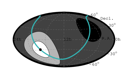
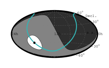
Figure 3: Contour plots of the (projected) number density of $\gamma$-ray sources in equatorial coordinates. The left hand panel refers to a model with $\rho\propto r^{-1}$ at the centre $(p,c)=(2,1/2)$, while the right-hand panel to a model with $\rho\propto r^{-7/4}$ at the centre $(p,c)=(1/2,1/2)$. The grey-scale gives the relative number density, with white representing the highest values and black the lowest. The number density changes by a factor of 10 on moving from one contour to the next. The Galactic centre and the Galactic plane are marked.

The circular speed and the cumulative mass can be found as

$$v_{\mathrm{c}}^{2}=-r\frac{\mathrm{d}\psi}{\mathrm{d}r}=\frac{cr^{p/2}+r^{p}}{(1+2cr^{p/2}+r^{p})^{1/p+1}},$$ (18)

$$M_{r}=rv_{\mathrm{c}}^{2}=\frac{1+cr^{-p/2}}{(1+2cr^{-p/2}+r^{-p})^{1/p+1}}.$$ (19)

Here, the total mass is finite and therefore the circular speed falls off as Keplerian at large radii ($v_{\mathrm{c}}\sim r^{-1/2}$). Fig. 2 shows plots of the circular velocity as a function of $r/r_{1/2}$, where $r_{1/2}$ is the half-mass radius, (i.e., $M_{r_{1/2}}=1/2$). The models with inner density slopes $\rho\propto r^{-1}$ or $\rho\propto r^{-3/2}$ have rotation curves similar to that of the NFW profile or Moore et al. (1998) models, and so are flattish over a wide range of radii.

The velocity dispersions are

$$\langle v_{r}^{2}\rangle=\frac{1+c^{2}+cg}{2(1+c^{2}+cg)+p(2+cg)}\,\psi,$$ (20)

$$\langle v_{\mathrm{T}}^{2}\rangle=\frac{p}{2}\frac{2+cg}{2(1+c^{2}+cg)+p(2+cg)}\,\psi,$$ (21)

where $g=r^{p/2}+r^{-p/2}$ and therefore the anisotropy parameter varies according to

$$\beta=1-\frac{p}{4}\,\left(\frac{2+cg}{1+c^{2}+cg}\right).$$ (22)

From its construction, the hypervirial relation is automatically satisfied. Because the potential is everywhere finite, the hypervirial relation also implies that the velocity dispersions are everywhere finite. In particular, assuming $c\neq 0$, the central velocity dispersions are $\langle v_{r}^{2}\rangle=1/(p+2)$ and $\langle v_{\mathrm{T}}^{2}\rangle=p/[2(p+2)]$. In addition,

$$\frac{d\beta}{dr}=\frac{p^{2}c(1-c^{2})r^{p/2-1}(r^{p}-1)}{8(c+r^{p/2})^{2}(1+cr^{p/2})^{2}},$$ (23)

and therefore, provided that $0<c<1$, the anisotropy parameter $\beta$ decreases from $\beta=1-p/4$ at $r=0$ to $\beta=1-p/[2(1+c)]$ at $r=1$ and then increases back to $\beta\rightarrow 1-p/4$ as $r\rightarrow\infty$. In other words, in this model, the velocity dispersions are more radially anisotropic near the centre and the outskirts whereas they are relatively less radially anisotropic around the region of the radial scalelength. However, we also note that the model as a whole always possesses a more radially biased velocity dispersion than the isotropic model unless $p>2(1+c)$.

It has been suggested that dark matter haloes achieve an almost isotropic state near the centre and become more and more radially anisotropic in the outer parts, at least according to cosmological N-body simulations (Hansen & Moore 2006). Our DFs are radially anisotropic and therefore better suited to modelling the outer parts and envelopes of dark haloes. They are unsuitable for the class of problems in which central anisotropy plays a critical role.

Figure 4: The distribution of line of sight velocities and proper motions of dark matter particles towards the Galactic Centre (upper panels), the anti-Centre (middle panels) and the Galactic North Pole (lower panels). The left-hand panels refer to the model with $(p,c)=(2,1/2)$, while the right-hand panels refer to the model with $(p,c)=(1/2,1/2)$. The velocity is given in units of $v_{0}=(GM/r_{0})^{1/2}$.

4 An application: the distribution of $\gamma$-ray sources

Diemand, Moore, & Stadel (2005) have presented evidence from numerical simulations that dark matter may be clumped into mini-haloes of Earth mass and larger. They estimate that $\sim$50% of the total mass of the dark matter halo is bound to dark matter substructures. These objects may be detectable by virtue of the $\gamma$-rays from neutralino annihilation in the very centres of the clumps. Diemand et al. (2005) also point out that the nearest mini-haloes will be amongst the very brightest sources from neutralino annihilation and may be found either with the forthcoming GLAST satellite or next-generation atmospheric Čerenkov telescopes as high proper motion, discrete $\gamma$-ray sources.

If this idea is correct, then there are some immediate consequences. First, because of the offset of the Sun’s location from the centre of the dark halo, the distribution of such $\gamma$-ray sources is anisotropic and the magnitude of the anisotropy is an indicator of the cusp slope at the Galactic Centre. This effect is already well-known in studies of halo origin of the ultra-high energy cosmic rays (e.g., Evans, Ferrer, & Sarkar 2002). Let us use Galactic coordinates $(s,\ell,b)$, where $s=|\@vec{s}|$ is heliocentric distance, and $(\ell,b)$ are Galactic longitude and latitude. Then, the relative number density of $\gamma$-ray sources is

$$F(\ell,b)\propto\int\!s^{2}\,\mathrm{d}s\,w(s)\,\rho[\@vec{R}_{\sun}+\@vec{s}_{\ell,b}]$$ (24)

where $\@vec{R}_{\sun}$ is the Galactocentric solar position and $w(s)$ is the selection function. For bright sources, the selection function is proportional to the relative luminosity and so $w(s)\propto s^{-2}$. The density profile is truncated at a radius at which the dark matter annihilation rate matches the collapse timescale of the cusp. With this assumption, a tiny constant density core is created (e.g., Tyler 2002) and convergence of the integral (24) is guaranteed. The overall normalization of the integral depends on the fraction of dark matter bound in mini-haloes, as opposed to smoothly distributed dark matter. The anisotropy effect is clearly illustrated in Fig. 3, which shows Hamer-Aitoff projections in equatorial coordinates for two of the halo models. The first is a model with $\rho\propto r^{-1}$ at the centre $(p,c)=(2,1/2)$, and the second is a model with $\rho\propto r^{-7/4}$ at the centre $(p,c)=(1/2,1/2)$. The more highly cusped the model, the greater the anisotropy. If there are enough detections, the magnitude of the anisotropy can be quantified by harmonic analysis (see e.g., Evans et al. 2002).

Second, if the high proper motion sources can be identified, this will provide the first direct evidence on the velocity distribution of the dark matter. It is therefore useful to have predictions of the velocity distributions. The proper motion and radial velocity distribution of dark matter clumps can be calculated easily for our models, because the DFs are simple. The proper motion and radial velocity distributions in direction $\mathrm{d}^{2}\Omega=\cos b\,\mathrm{d}\ell\,\mathrm{d}b$ is

$$\frac{\mathrm{d}^{2}N_{\mathrm{obs}}}{\mathrm{d}v_{\ell}\mathrm{d}v_{b}}(v_{\ell},v_{b},\ell,b)=\mathrm{d}^{2}\!\Omega\iint\!\mathrm{d}v_{s}\,\mathrm{d}s\ f(E,L)\,s^{2}\,w(s),$$ (25)

$$\frac{\mathrm{d}N_{\mathrm{obs}}}{\mathrm{d}v_{s}}(v_{s},\ell,b)=\mathrm{d}^{2}\!\Omega\iiint\!\mathrm{d}v_{\ell}\,\mathrm{d}v_{b}\,\mathrm{d}s\ f(E,L)\,s^{2}\,w(s).$$ (26)

Here, the velocity of the dark matter particles has been resolved into components $(v_{s},v_{\ell},v_{b})$ based on Galactic coordinates while $f(E,L)$ is the DF of the dark matter. For models with DFs (2), the above triple integrals are easily computed via Gaussian quadrature. In fact, the second moments of these distributions are entirely analytic, as sketched out in Appendix A. Fig. 4 shows the proper motion and line of sight velocity distributions for the dark matter clumps in three directions. When looking towards the Galactic Centre or anti-Centre in spherical models, then the distributions of the two tangential velocity components $v_{\ell}$ and $v_{b}$ are the same, though this is not necessarily the case in other directions. All three velocity distributions show very significant deviations from Gaussianity. The sources with highest tangential velocity occur towards the the Galactic Centre direction and it is therefore in this direction that GLAST or VERITAS may find it easiest to detect them unambiguously.

Although these facts have been established in the context of our simple family of models, we argue that they are likely to be generic. The anisotropy effect in source positions is a consequence of the Sun’s offset from the centre. The fastest moving sources are likely to be found in the direction in which the gravitational potential well is deepest.

5 Conclusions

We have presented a simple family of halo models useful for the study of dark matter haloes. They have a simple potential and distribution function (DF), being composed of two terms of the form of $L^{p-2}E^{(3p+1)/2}$ – where $L$ is the total angular momentum, $E$ the binding energy and $p$ is some constant. As an application, we have presented the properties of discrete $\gamma$-ray sources arising from neutralino annihilation in dark matter mini-haloes. This suggestion for the composition of the dark matter is derived the numerical simulations of Diemand et al. (2005). If true, then nearby, high proper motion discrete $\gamma$-rays sources may be detectable by forthcoming missions such as GLAST. We have shown that there is an anisotropy in the positions of such $\gamma$-ray sources because of the offset of the Sun from the Galactic Centre. We have also provided distributions of proper motions and line of sight velocities of such sources. The best direction in which to look is towards the Galactic Centre $(\ell,b)=(0,0)$. There are more sources in this direction and they have the highest proper motion.

This paper also continues the study of hyperviriality begun by Eddington (1916) and further developed by Evans & An (2005). In spherical symmetry, any model which has a DF that is a sum of terms like $L^{p-2}E^{(3p+1)/2}$ is hypervirial. This leads to the derivation of a general differential equation that any spherical hypervirial system must satisfy. We have solved it to find the most general models, for which the potential can be written down in terms of elementary functions.

We briefly note that, in the case of axisymmetry, any model which has a DF that is a sum of terms like $L_{z}^{p-2}E^{(3p+1)/2}$ – where $L_{z}$ is the angular momentum component about the axis of symmetry – is also hypervirial (see Appendix B for more details). It is possible to derive the equation for the corresponding potential and demonstrate that at least two analytical solutions exist, corresponding to the flattened Plummer model studied by Lynden-Bell (1962) and a particular case among the prolate galaxy models of Lake (1981). In fact, only the Plummer model – the sole isotropic, hypervirial model – can be generalized to give an axisymmetric hypervirial system. It is an open question whether any further hypervirial generalizations of the Plummer model can be found.

Appendix A Second moments of the velocity distributions

It is straightforward to compute the six independent components of the velocity dispersion tensor in a Galactic coordinate system. These formulae do not appear to have been given before, and so we quote them here:

$$\langle v_{s}^{2}\rangle = \langle v_{x}^{2}\rangle\cos^{2}\!b\,\cos^{2}\!\ell+\langle v_{y}^{2}\rangle\cos^{2}\!b\,\sin^{2}\!\ell+\langle v_{z}^{2}\rangle\sin^{2}\!b+\langle v_{x}v_{y}\rangle\cos^{2}\!b\,\sin 2\ell-\langle v_{y}v_{z}\rangle\sin 2b\,\sin\ell-\langle v_{x}v_{z}\rangle\sin 2b\,\cos\ell,$$ (27)

$$\langle v_{b}^{2}\rangle = \langle v_{x}^{2}\rangle\sin^{2}\!b\,\cos^{2}\!\ell+\langle v_{y}^{2}\rangle\sin^{2}\!b\,\sin^{2}\!\ell+\langle v_{z}^{2}\rangle\cos^{2}\!b+\langle v_{x}v_{y}\rangle\sin^{2}\!b\,\sin 2\ell+\langle v_{y}v_{z}\rangle\sin 2b\,\cos\ell+\langle v_{x}v_{z}\rangle\sin 2b\,\sin\ell,$$ (28)

$$\langle v_{\ell}^{2}\rangle = \langle v_{x}^{2}\rangle\sin^{2}\!\ell+\langle v_{y}^{2}\rangle\cos^{2}\!\ell-\langle v_{x}v_{y}\rangle\sin 2\ell,$$ (29)

$$\langle v_{s}v_{b}\rangle = -\langle v_{x}^{2}\rangle\cos b\,\sin b\,\cos^{2}\!\ell-\langle v_{y}^{2}\rangle\cos b\,\sin b\,\sin^{2}\!\ell+\langle v_{z}^{2}\rangle\cos b\,\sin b-\langle v_{x}v_{y}\rangle\sin 2b\,\cos\ell\,\sin\ell$$ (31)

$$-\langle v_{x}v_{z}\rangle\cos 2b\,\cos\ell-\langle v_{y}v_{z}\rangle\cos 2b\,\sin\ell,$$

$$\langle v_{\ell}v_{s}\rangle = \langle v_{y}^{2}-v_{x}^{2}\rangle\cos b\,\sin\ell\,\cos\ell+\langle v_{x}v_{y}\rangle\cos b\,\cos 2\ell+\langle v_{x}v_{z}\rangle\sin b\,\sin\ell-\langle v_{y}v_{z}\rangle\sin b\,\cos\ell,$$ (32)

$$\langle v_{\ell}v_{b}\rangle = \langle v_{x}^{2}-v_{y}^{2}\rangle\sin b\,\sin\ell\,\cos\ell-\langle v_{x}v_{y}\rangle\cos b\,\cos 2\ell+\langle v_{x}v_{z}\rangle\cos b\,\sin\ell-\langle v_{y}v_{z}\rangle\cos b\,\cos\ell.$$ (33)

This gives the observables in terms of the second moments referred to Cartesian coordinates. The latter can be related to the second moments in spherical polars (in which the tensor diagonalizes) via:

$$\langle v_{x}^{2}\rangle=\frac{x^{2}}{r^{2}}\langle v_{r}^{2}\rangle+\frac{y^{2}+z^{2}}{r^{2}}\langle v_{\theta}^{2}\rangle,\qquad\langle v_{y}^{2}\rangle=\frac{y^{2}}{r^{2}}\langle v_{r}^{2}\rangle+\frac{x^{2}+z^{2}}{r^{2}}\langle v_{\theta}^{2}\rangle,\qquad\langle v_{z}^{2}\rangle=\frac{z^{2}}{r^{2}}\langle v_{r}^{2}\rangle+\frac{x^{2}+y^{2}}{r^{2}}\langle v_{\theta}^{2}\rangle,$$ (34)

$$\langle v_{x}v_{y}\rangle=\frac{xy}{r^{2}}\left(\langle v_{r}^{2}\rangle-\langle v_{\theta}^{2}\rangle\right),\qquad\langle v_{x}v_{z}\rangle=\frac{xz}{r^{2}}\left(\langle v_{r}^{2}\rangle-\langle v_{\theta}^{2}\rangle\right),\qquad\langle v_{y}v_{z}\rangle=\frac{yz}{r^{2}}\left(\langle v_{r}^{2}\rangle-\langle v_{\theta}^{2}\rangle\right).$$ (35)

Here, $\langle v_{\theta}^{2}\rangle=\langle v_{\phi}^{2}\rangle=\langle v_{\mathrm{T}}^{2}\rangle/2$. Hence, by substituting in the known velocity dispersions in spherical polars (Eqs. 20 and 21), we obtain the second moments of the observable distributions (the line of sight velocities and the proper motions).

Appendix B Axisymmetric hypervirial potentials

Upon the discovery of the new hypervirial potential, one may ask the question: does there exist a simple extension of the spherical hypervirial potentials into axisymmetry? A possible starting point of the investigation is the examination of axisymmetric DFs that are obtained by replacing the $L$-dependence of a spherically symmetric DF with an $L_{z}$-dependence. Let us suppose that the DF of an axisymmetric system is given by

$$f(E,L_{z})=C|L_{z}|^{2n}E^{m-3/2},$$ (36)

where $L_{z}=Rv_{\phi}$ is the angular momentum along the symmetry axis, and $n>-1/2$ and $m>1/2$. Then, a simple integration leads to the expressions for the corresponding density (c.f., Fricke 1952; Dejonghe 1986; Evans 1994)

$$\rho=2^{n+3/2}\piup C\frac{\Gamma(n+1/2)\Gamma(m-1/2)}{\Gamma(n+m+1)}R^{2n}\psi^{n+m},$$ (37)

and the second-order velocity moments

$$\rho\langle v_{R}^{2}\rangle=2^{n+3/2}\piup C\frac{\Gamma(n+1/2)\Gamma(m-1/2)}{\Gamma(n+m+2)}R^{2n}\psi^{n+m+1}=\frac{\rho\psi}{n+m+1}\,;$$

$$\rho\langle v_{\phi}^{2}\rangle=2^{n+5/2}\piup C\frac{\Gamma(n+3/2)\Gamma(m-1/2)}{\Gamma(n+m+2)}R^{2n}\psi^{n+m+1}=(2n+1)\rho\langle v_{R}^{2}\rangle.$$ (38)

Note that $\rho\langle v_{R}^{2}\rangle=\rho\langle v_{z}^{2}\rangle=\rho\langle v_{r}^{2}\rangle=\rho\langle v_{\theta}^{2}\rangle$ since the DF is symmetric with respect to $v_{R}\leftrightarrow v_{z}$ exchange. Finally, we find that, for the system described by the DF of Eq. (36),

$$\rho\langle v^{2}\rangle=\rho\left(\langle v_{R}^{2}\rangle+\langle v_{z}^{2}\rangle+\langle v_{\phi}^{2}\rangle\right)=(2n+3)\rho\langle v_{R}^{2}\rangle=\frac{2n\!+\!3}{n\!+\!m\!+\!1}\ \rho\psi,$$ (39)

and thus that the steady-state virial theorem holds without the boundary terms only if $m=3n+5$, for which the system becomes hypervirial. Here, the density of the system (Eq. 37) is axisymmetric, but there is no net rotation ($\langle v_{\phi}\rangle=0$), as the DF (36) is symmetric with respect to $L_{z}\leftrightarrow-L_{z}$ exchange. To rectify this, we can amend the DF (36) by

$$f(E,L_{z})=C\left[1+\xi(L_{z})\right]|L_{z}|^{2n}E^{m-3/2}$$ (40)

where $\xi(L_{z})$ is an arbitrary odd function of $L_{z}$ [i.e, $\xi(-L_{z})=-\xi(L_{z})$] that is bounded by $-1\leq\xi(L_{z})\leq 1$. Note that, on the ground of statistical mechanics, Dejonghe (1986, 1987) advocated the form of $\xi(L_{z})$ being $\tanh(kL_{z})$ where $k$ is a parameter that depends on the total angular momentum along the symmetry axis. Physically, this action of adding a certain odd function to the even distribution function corresponds to switching the direction of rotations for a certain fraction of stars of given $|L_{z}|$ and $E$. It is straightforward to show that, for the DF of Eq. (40), Eqs. (37) and (38) are still true while

$$\rho\langle v_{\phi}\rangle=\int\!v_{\phi}f\,\mathrm{d}^{3}\!\@vec{v} = \frac{4\piup C}{2m-1}\,\int_{-\sqrt{2\psi R^{2}}}^{\sqrt{2\psi R^{2}}}\!\frac{\mathrm{d}L_{z}}{R^{2}}\,L_{z}\left[1+\xi(L_{z})\right]\left(L_{z}^{2}\right)^{n}\left(\psi-\frac{L_{z}^{2}}{2R^{2}}\right)^{m-1/2}$$

$$= \frac{2^{n+3}\piup C}{2m-1}\,R^{2n}\psi^{n+m+1/2}\int_{0}^{1}\!\xi\left(\sqrt{2\psi R^{2}t}\right)\,t^{n}\left(1-t\right)^{m-1/2}\,\mathrm{d}t$$

$$\leq 2^{n+2}\piup C\frac{\Gamma(n+1)\Gamma(m-1/2)}{\Gamma(n+m+3/2)}R^{2n}\psi^{n+m+1/2}=2^{1/2}\frac{\Gamma(n+1)\Gamma(n+m+1)}{\Gamma(n+1/2)\Gamma(n+m+3/2)}\rho\psi^{1/2}.$$

In other words, one can choose $\xi(L_{z})$ to meet the constraint on the net rotation $\langle v_{\phi}\rangle$. Here, the inequality becomes the equality if $\xi(L_{z})=1$ for $L_{z}>0$, which corresponds to the situation when every star rotates in the same direction. For $n>-1/2$ and $m=3n+5$, it is straightforward to established that $\langle v_{\phi}\rangle^{2}<\psi/2$.

Systems given by the DF (36) are somewhat unrealistic since the density along the symmetry axis is either zero ($n>0$) or infinite ($n<0$) except the $n=0$ case that is just the isotropic (and spherically symmetric) Plummer model. However, analogous to the procedure in Sect. 2, we may obtain more realistic systems by summing DFs of the form of Eq. (36), one of which corresponds to that of the isotropic Plummer model, that is,

$$f(E,L_{z})=C_{0}E^{7/2}+\sum_{i}C_{i}|L_{z}|^{2n_{i}}E^{3n_{i}+7/2}+f_{\mathrm{odd}}(E,L_{z})$$ (41)

where each $n_{i}$ should be positive in order to avoid the divergent behaviour of the density along the symmetry axis. Here, $f_{\mathrm{odd}}(E,L_{z})$ is an arbitrary function that satisfies the condition that $f_{\mathrm{odd}}(E,-L_{z})=-f_{\mathrm{odd}}(E,L_{z})$ and chosen so that the $f(E,L_{z})$ is non-negative for all accessible $E$ and $L_{z}$. It is a simple exercise to find expressions for the density

$$\rho=D_{0}\psi^{5}+\sum_{i}D_{i}R^{2n_{i}}\psi^{4n_{i}+5}\,;\qquad D_{0}=\frac{7\piup^{2}}{2^{11/2}}C_{0}\,;\qquad D_{i}=2^{n_{i}+3/2}\piup C_{i}\frac{\Gamma(n_{i}+1/2)\Gamma(3n_{i}+9/2)}{\Gamma(4n_{i}+6)},$$ (42)

and the second-order velocity moments

$$\rho\langle v_{R}^{2}\rangle=\frac{D_{0}}{6}\psi^{6}+\sum_{i}\frac{D_{i}}{2(2n_{i}+3)}\ R^{2n_{i}}\psi^{4n_{i}+6}\,;\qquad\rho\langle v_{\phi}^{2}\rangle=\frac{D_{0}}{6}\psi^{6}+\sum_{i}\frac{(2n_{i}+1)D_{i}}{2(2n_{i}+3)}\ R^{2n_{i}}\psi^{4n_{i}+6}.$$ (43)

It is also easy to establish that the system is in fact hypervirial,

$$\rho\langle v^{2}\rangle=\rho\left(2\langle v_{R}^{2}\rangle+\langle v_{\phi}^{2}\rangle\right)=\frac{D_{0}}{2}\psi^{6}+\sum_{i}\frac{D_{i}}{2}\ R^{2n_{i}}\psi^{4n_{i}+6}=\rho\frac{\psi}{2}.$$ (44)

However, finding the corresponding potential is actually a non-trivial problem as it is tantamount to solving Poisson’s equation, which now becomes a second-order partial differential equation:

$$\frac{1}{r^{2}}\frac{\partial}{\partial r}\left(r^{2}\frac{\partial\psi}{\partial r}\right)+\frac{1}{r^{2}\sin\theta}\frac{\partial}{\partial r}\left(\sin\theta\frac{\partial\psi}{\partial\theta}\right)=-4\piup D_{0}\psi^{5}-4\piup\sum_{i}D_{i}r^{2n_{i}}\sin^{2n_{i}}\!\theta\,\psi^{4n_{i}+5}$$ (45)

in the spherical polar coordinate system or

$$\frac{1}{R}\frac{\partial}{\partial R}\left(R\frac{\partial\psi}{\partial R}\right)+\frac{\partial^{2}\psi}{\partial z^{2}}=-4\piup D_{0}\psi^{5}-4\piup\sum_{i}D_{i}R^{2n_{i}}\psi^{4n_{i}+5}$$ (46)

in the cylindrical polar coordinate system. Even after factoring out the scalefree contribution (c.f, Toomre 1982),

$$\frac{\partial^{2}\varphi}{\partial t^{2}}+\cosh^{2}\!\zeta\,\frac{\partial^{2}\varphi}{\partial\zeta^{2}}-\frac{\varphi}{4}=-4\piup D_{0}\varphi^{5}-4\piup\sum_{i}D_{i}\frac{\varphi^{4n_{i}+5}}{\cosh^{2n_{i}}\!\zeta}$$ (47)

where $\varphi=r^{1/2}\psi$, $t=\ln r$, and $\cos\theta=\tanh\zeta$ or

$$R^{2}\left(\frac{\partial^{2}\phi}{\partial R^{2}}+\frac{\partial^{2}\phi}{\partial z^{2}}\right)+\frac{\phi}{4}=-4\piup D_{0}\phi^{5}-4\piup\sum_{i}D_{i}\phi^{4n_{i}+5}$$ (48)

where $\phi=R^{1/2}\psi$, these are not obviously separable in either coordinate system. Instead, here, we take a rather different approach. Inspired by Eq. (15), we first consider the axisymmetric potential of the form of

$$\psi=\frac{1}{[1+c(\theta)r^{p/2}+r^{p}]^{1/p}}$$ (49)

where $c(\theta)$ is some function of the latitude $\theta$. Then, the corresponding density can be found to be ($G=1$)

$$\rho=-\frac{1}{4\piup}\nabla^{2}\psi=(p+1)\left[1-\frac{c^{2}}{4}-\left(\frac{1}{p}\frac{\mathrm{d}c}{\mathrm{d}\theta}\right)^{2}\right]r^{p-2}\psi^{2p+1}+\frac{1}{p}\left[\frac{1}{\sin\theta}\frac{\mathrm{d}}{\mathrm{d}\theta}\left(\sin\theta\frac{\mathrm{d}c}{\mathrm{d}\theta}\right)+\frac{p(p+2)}{4}c\right]r^{p/2-2}\psi^{p+1}.$$ (50)

Now, we find that one of the necessary condition for the system to be consistent with the hypervirial DF is that $c(\theta)$ is the solution of the inhomogeneous Legendre equation

$$\frac{1}{\sin\theta}\frac{\mathrm{d}}{\mathrm{d}\theta}\left(\sin\theta\frac{\mathrm{d}c}{\mathrm{d}\theta}\right)+\frac{p}{2}\left(\frac{p}{2}+1\right)c=pC\sin^{p/2-2}\!\theta$$ (51)

where $C$ is a non-negative constant. A simple trial reveals that $c_{0}=4Cp^{-1}\sin^{p/2}\!\theta$ is its particular solution, and so the general solution is

$$c=AP_{p/2}(\cos\theta)+BQ_{p/2}(\cos\theta)+\frac{4C}{p}\sin^{p/2}\!\theta$$ (52)

where $P_{l}(x)$ is the Legendre-P function (polynomial if $l$ is an integer), $Q_{l}(x)$ is the Legendre-Q function, and $A$ and $B$ are the integration constants. Finally, the system can be hypervirial only if

$$1-\frac{c^{2}}{4}-\left(\frac{1}{p}\frac{\mathrm{d}c}{\mathrm{d}\theta}\right)^{2}\propto\sin^{p-2}\!\theta$$ (53)

where $c$ is given by Eq. (52). It is rather obvious that we only need to examine the cases when $p/2$ is an integer and $B=0$. After a further examination, we find that, only possible cases are $p=4$

$$c(\theta)=3\cos^{2}\!\theta-1+C\sin^{2}\!\theta=2+(C-3)\sin^{2}\!\theta\,;\qquad\psi=\frac{1}{[1+2r^{2}+r^{4}+(C-3)R^{2}]^{1/4}},$$ (54)

and $p=2$

$$c(\theta)=A\cos\theta+2C\sin\theta\,;\qquad\psi=\frac{1}{[1+r^{2}+Az+2CR]^{1/2}}$$ (55)

where $A^{2}\leq 4(1-C^{2})$. The corresponding densities for both cases reduce the form of Eq. (42). In fact, the potential corresponding to both solutions are already known!

The first ($p=4$) is the flattened Plummer model of Lynden-Bell (1962),

$$\psi=\frac{\psi_{0}a}{[(r^{2}+a^{2})^{2}-2b^{2}R^{2}]^{1/4}}\,;\qquad\rho=\frac{\psi_{0}(3-2\epsilon)}{\piup Ga^{2}}\left(\frac{\psi}{\psi_{0}}\right)^{5}+\frac{5\psi_{0}\epsilon(2-\epsilon)}{\piup Ga^{2}}\left(\frac{R}{a}\right)^{2}\left(\frac{\psi}{\psi_{0}}\right)^{9}$$ (56)

where $0\leq\epsilon=b^{2}/a^{2}\leq 3/2$. Comparing this to Eq. (42), we find that the DF

$$f_{\mathrm{even}}(E,L_{z})=C_{0}E^{7/2}+C_{1}L_{z}^{2}E^{13/2}\,;\qquad C_{0}=\frac{2^{11/2}}{7\piup^{3}}\ \frac{3-2\epsilon}{Ga^{2}\psi_{0}^{4}}\,;\qquad C_{1}=\frac{2^{25/2}\cdot 3\cdot 5}{11\cdot 13\piup^{3}}\ \frac{\epsilon(2-\epsilon)}{Ga^{4}\psi_{0}^{8}}$$ (57)

can build the potential-density pair of the flattened Plummer model. The second-order velocity moments are

$$\rho\langle v_{R}^{2}\rangle=\frac{\psi_{0}^{2}(3-2\epsilon)}{6\piup Ga^{2}}\ \left(\frac{\psi}{\psi_{0}}\right)^{6}+\frac{\psi_{0}^{2}\epsilon(2-\epsilon)}{2\piup Ga^{2}}\ \left(\frac{R}{a}\right)^{2}\left(\frac{\psi}{\psi_{0}}\right)^{10}\,;\qquad\rho\langle v_{\phi}^{2}\rangle=\frac{\psi_{0}^{2}(3-2\epsilon)}{6\piup Ga^{2}}\ \left(\frac{\psi}{\psi_{0}}\right)^{6}+\frac{3\psi_{0}^{2}\epsilon(2-\epsilon)}{2\piup Ga^{2}}\ \left(\frac{R}{a}\right)^{2}\left(\frac{\psi}{\psi_{0}}\right)^{10},$$ (58)

and the system is hypervirial, as already noted by Lynden-Bell (1962).

The second ($p=2$) is a particular case of the generalized Plummer model devised by Lake (1981), for which

$$\psi=\frac{\psi_{0}a}{[r^{2}+a^{2}+2bR]^{1/2}}\,;\qquad\rho=\frac{3\psi_{0}(1-\epsilon^{2})}{4\piup Ga^{2}}\left(\frac{\psi}{\psi_{0}}\right)^{5}+\frac{\psi_{0}\epsilon}{4\piup Ga^{2}}\left(\frac{a}{R}\right)\left(\frac{\psi}{\psi_{0}}\right)^{3}$$ (59)

where $0\leq\epsilon=b/a\leq 1$. This reduces to Eq. (54) after an arbitrary translation along the symmetry axis ($R=0$). In fact, this is singular on the entire $R=0$ axis and so best represents prolate galaxies. The DF is

$$f_{\mathrm{even}}(E,L_{z})=C_{0}E^{7/2}+C_{1}\delta(L_{z})E^{2}\,;\qquad C_{0}=\frac{2^{7/2}\cdot 3}{7\piup^{3}}\ \frac{1-\epsilon^{2}}{Ga^{2}\psi_{0}^{4}}\,;\qquad C_{1}=\frac{3}{8\piup^{2}}\frac{\epsilon}{Ga\psi_{0}^{2}}.$$ (60)

Note that the Dirac-$\delta$ distribution is the limiting case of Eq. (36) as in $\lim_{n\rightarrow(-1/2)}[|L_{z}|^{2n}/\Gamma(n+1/2)]=\delta(L_{z})$. The second-order velocity moments are

$$\rho\langle v_{R}^{2}\rangle=\frac{\psi_{0}^{2}(1-\epsilon^{2})}{8\piup Ga^{2}}\left(\frac{\psi}{\psi_{0}}\right)^{6}+\frac{\psi_{0}^{2}\epsilon}{16\piup Ga^{2}}\left(\frac{a}{R}\right)\left(\frac{\psi}{\psi_{0}}\right)^{4}\,;\qquad\rho\langle v_{\phi}^{2}\rangle=\frac{\psi_{0}^{2}(1-\epsilon^{2})}{8\piup Ga^{2}}\left(\frac{\psi}{\psi_{0}}\right)^{6},$$ (61)

and so this model is hypervirial.

The existence of the flattened Plummer models poses the question as to whether there are axisymmetric generalizations with simple DFs for all the hypervirial models. We argue that this is not the case because the Plummer model is the only isotropic hypervirial model. Any DF of $f(E,L)$ of a spherically symmetric system has degenerate velocity dispersions in the tangential plane, while any DF $f(E,L_{z})$ of a axisymmetric system has the velocity dispersions within the meridional plane degenerate. Clearly, only the isotropic case can have both the tangential plane and meridional plane as planes of symmetry of the local velocity ellipsoid. This, therefore, implies that, if the flattening method, however it is chosen, is gradual in the sense that it includes the spherically symmetric case as a particular case, the corresponding DF should necessarily reduce to not only a spherically symmetric but also an isotropic DF of $f(E)$. In other words, only those spherically symmetric potentials with a simple isotropic DF can have an axisymmetric family of its generalization with continuous values of flattening parameters. This, of course, does not rule out the possibility that with a very special values of flattening parameters, the corresponding DF may be simple but there would not be any continuous transitions to the spherically symmetric case while maintaining the simplicity of the DF.

Appendix C General solutions of generalized Lane-Emden equation

The differential equation in Eq. (6) when the sum contains only a single term is a particular case of a family of differential equations investigated by Goenner & Havas (2000), which they called the generalized Lane-Emden equation. In fact, Eq. (6) corresponds to the special case of parameter combinations noted by them (see eq. 11 of Goenner & Havas 2000) that permits a rational transformation of variables that leaves the differential equation form-invariant. The one-parameter solution family (eq. 18 of Goenner & Havas 2000) is the direct generalization of the Schuster-Emden integral (see e.g. Horedt 1986) and corresponds to the solution for the case of $A=0$ in Eq. (10), which leads to the models of Evans & An (2005).

If we consider a transformation, $\eta=\varphi^{s}$, Eq. (10) with a single term in the sum further reduces to

$$\left(\frac{\mathrm{d}\eta}{\mathrm{d}t}\right)^{2}=As^{2}\eta^{2-2/s}+\frac{s^{2}}{4}\eta^{2}-Bs^{2}\eta^{2+2p/s}.$$ (62)

We note that the differential equation of the form of $(y^{\prime})^{2}=f(y)$ where $f(y)$ is a cubic or quartic polynomial of $y$ can be solved with standard elliptic functions. Here, for $AB\neq 0$, the right-hand side of Eq. (62) can become a cubic of quartic polynomial of $\eta$ if $s=\pm 1$ (with $p=1$ or $p=2$) or $s=\pm 2$ (with $p=1/2$ or $p=1$). In other words, the two-parameter general solutions of Eq. (6), or equivalently the solutions of Eq. (10) with $A\neq 0$ can be written down in closed form using elliptic functions if the sum contains a single term with $p=$1/2, 1, or 2 (Goenner & Havas 2000).

C.1 Solutions in terms of Weierstrass-P functions

Let us be reminded that the Weierstrass-P function is the canonical elliptic function (i.e., complex bi-periodic meromorphic function) with second-order poles. It is usually defined in terms of the sum over the lattice points in complex plane with two half-periods. However, for our purpose, it is useful to consider the differential equation

$$\left[\frac{\mathrm{d}}{\mathrm{d}z}\wp(z;g_{2},g_{3})\right]^{2}=4[\wp(z;g_{2},g_{3})]^{3}-g_{2}\wp(z;g_{2},g_{3})-g_{3}$$ (63)

that is satisfied by $\wp(z;g_{2},g_{3})$. Here, $g_{2}$ and $g_{3}$ are usually referred to as elliptic invariants. We further note that the differential equation (63) does not explicitly involve the independent variable so that one integration constant is given by an arbitrary translation, that is, if $\varphi(t)$ is its solution, then $\varphi(t+c)$ where $c$ is an arbitrary (complex) constant is also the solution. However, Eq. (63) is a first order differential equation, and thus, $\wp(z+c;g_{2},g_{3})$ is indeed the complete specification of its general solution. In addition, the above differential equation also indicates that $\wp$-function is homogeneous, i.e.,

$$\wp(\lambda z;g_{2},g_{3})=\lambda^{-2}\wp(z;\lambda^{4}g_{2},\lambda^{6}g_{3}).$$ (64)

The right-hand side of Eq. (62) becomes a cubic polynomial if i) $B\neq 0$, $s=2p$ ($p=1/2$ or 1) or ii) $A\neq 0$, $s=-2$ ($p=1$ or 2). For these cases, linear transformations $\eta=\lambda(\zeta+\tau)$ with properly chosen $\lambda$ and $\tau$ can reduce Eq. (62) to the form of Eq. (63). After a bit of algebra, we find solutions of Eq. (10) (see also Goenner & Havas 2000);

$$\varphi=\frac{1}{B}\left[\frac{1}{2^{2}\cdot 3}-2^{2}\wp\left(t+c;\,\frac{1}{2^{6}\cdot 3},\,-\frac{AB^{2}}{2^{4}}-\frac{1}{2^{9}\cdot 3^{3}}\right)\right]\qquad\ \mbox{for }\ B\neq 0,\ p=1/2,$$ (65)

$$\varphi^{2}=\frac{1}{B}\left[\frac{1}{2^{2}\cdot 3}-\wp\left(t+c;\,2^{2}AB+\frac{1}{2^{2}\cdot 3},\,-\frac{AB}{3}-\frac{1}{2^{3}\cdot 3^{3}}\right)\right]\qquad\ \mbox{for }\ B\neq 0,\ p=1,$$ (66)

$$\varphi^{-2}=\frac{1}{A}\left[\wp\left(t+c;\,2^{2}AB+\frac{1}{2^{2}\cdot 3},\,-\frac{AB}{3}-\frac{1}{2^{3}\cdot 3^{3}}\right)-\frac{1}{2^{2}\cdot 3}\right]\qquad\ \mbox{for }\ A\neq 0,\ p=1,$$ (67)

$$\varphi^{-2}=\frac{1}{A}\left[\wp\left(t+c;\,\frac{1}{2^{2}\cdot 3},\,2^{2}A^{2}B-\frac{1}{2^{3}\cdot 3^{3}}\right)-\frac{1}{2^{2}\cdot 3}\right]\qquad\ \mbox{for }\ A\neq 0,\ p=2.$$ (68)

C.2 Solutions for $p=1$ in terms of Jacobi elliptic functions

The Jacobi elliptic functions are defined through the inverse function of the elliptic integral of the first kind, i.e.,

$$\mbox{sn}(u,k)=\sin\phi\,;\qquad\mbox{cn}(u,k)=\cos\phi\,;\qquad\mbox{dn}(u,k)=\sqrt{1-k^{2}[\mbox{sn}(u,k)]^{2}}$$ (69)

where

$$u=F(\phi,k)=\int_{0}^{\phi}\!\frac{\mathrm{d}t}{\sqrt{1-k^{2}\sin^{2}\!t}}=\int_{0}^{\mbox{sn}(u,k)}\!\frac{\mathrm{d}v}{(1-v^{2})^{1/2}(1-k^{2}v^{2})^{1/2}}$$ (70)

and $k$ is the elliptic modulus. Remaining elliptic functions are defined as

$$\begin{array}[]{lll}\mbox{ns}\,u\equiv\mbox{sn}\,u;&\mbox{nc}\,u\equiv\mbox{cn}\,u;&\mbox{nd}\,u\equiv\mbox{dn}\,u;\\ \mbox{sc}\,u\equiv\mbox{sn}\,u\ \mbox{nc}\,u;&\mbox{cd}\,u\equiv\mbox{cn}\,u\ \mbox{nd}\,u;&\mbox{ds}\,u\equiv\mbox{dn}\,u\ \mbox{ns}\,u;\\ \mbox{cs}\,u\equiv\mbox{ns}\,u\ \mbox{cn}\,u;&\mbox{dc}\,u\equiv\mbox{nc}\,u\ \mbox{dn}\,u;&\mbox{sd}\,u\equiv\mbox{nd}\,u\ \mbox{sn}\,u.\end{array}$$ (71)

Here, the common elliptic modulus $k$ is omitted following usual practices. The derivative of $\mbox{sn}\,u$ is given by

$$\frac{\mathrm{d}}{\mathrm{d}u}\,\mbox{sn}\,u=\mbox{cn}\,u\ \mbox{dn}\,u$$ (72)

and the derivatives of remaining elliptic functions can be found using their respective definitions and Eq. (72). Then, it is straightforward to show that each Jacobi elliptic function is a particular solution of second-order differential equations such that

$$\begin{array}[]{lll}(\mbox{sn}\,u)^{\prime\prime}=-(1+k^{2})\,\mbox{sn}\,u+2k^{2}\,\mbox{sn}^{3}u;&(\mbox{cn}\,u)^{\prime\prime}=(2k^{2}-1)\,\mbox{cn}\,u-2k^{2}\,\mbox{cn}^{3}u;&(\mbox{dn}\,u)^{\prime\prime}=(2-k^{2})\,\mbox{dn}\,u-2\,\mbox{dn}^{3}u;\\ (\mbox{ns}\,u)^{\prime\prime}=-(1+k^{2})\,\mbox{ns}\,u+2\,\mbox{ns}^{3}u;&(\mbox{nc}\,u)^{\prime\prime}=(2k^{2}-1)\,\mbox{nc}\,u+2(1-k^{2})\,\mbox{nc}^{3}u;&(\mbox{nd}\,u)^{\prime\prime}=(2-k^{2})\,\mbox{nd}\,u-2(1-k^{2})\,\mbox{nd}^{3}u;\\ (\mbox{cd}\,u)^{\prime\prime}=-(1+k^{2})\,\mbox{cd}\,u+2k^{2}\,\mbox{cd}^{3}u;&(\mbox{sd}\,u)^{\prime\prime}=(2k^{2}-1)\,\mbox{sd}\,u-2k^{2}(1-k^{2})\,\mbox{sd}^{3}u;&(\mbox{sc}\,u)^{\prime\prime}=(2-k^{2})\,\mbox{sc}\,u+2(1+k^{2})\,\mbox{sc}^{3}u;\\ (\mbox{dc}\,u)^{\prime\prime}=-(1+k^{2})\,\mbox{dc}\,u+2\,\mbox{dc}^{3}u;&(\mbox{ds}\,u)^{\prime\prime}=(2k^{2}-1)\,\mbox{ds}\,u+2\,\mbox{ds}^{3}u;&(\mbox{cs}\,u)^{\prime\prime}=(2-k^{2})\,\mbox{cs}\,u+2\,\mbox{cs}^{3}u\end{array}$$ (73)

where the primed symbols indicate the differentiation with respect to the argument $u$ and the simplified notations for power (e.g., $\mbox{sn}^{3}u=[\mbox{sn}(u,k)]^{3}$ etc.) are used.

For Eq. (9) when the sum contains a single term with $p=1$;

$$\frac{\mathrm{d}^{2}\varphi}{\mathrm{d}t^{2}}=\frac{\varphi}{4}-2B\varphi^{3}$$ (74)

where $B=2\piup D$, we first note that it does not involves the independent variable explicitly, and therefore that, if $\varphi(t)$ is its solution, then $\varphi(t+c)$ where $c$ is an arbitrary constant is also the solution. That is, one of the integration constants of the general solution of Eq. (74) is related to arbitrary translation of a particular solution. Next, let us think of linear transformations of variables, $\varphi=\lambda\tilde{\varphi}$ and $\tilde{t}=\alpha(t-t_{0})$ where $t_{0}$ is an arbitrary integration constant while $\lambda$ and $\alpha$ are constants to be specified. With these new variables, Eq. (74) is transformed to

$$\frac{\mathrm{d}^{2}\tilde{\varphi}}{\mathrm{d}\tilde{t}^{2}}=\frac{1}{4\alpha^{2}}\tilde{\varphi}-2\frac{B\lambda^{2}}{\alpha^{2}}\tilde{\varphi}^{3},$$ (75)

which can reduce to any of the differential equations in Eq. (73) by proper choices of the constants. Note that there are two constants, $\lambda$ and $\alpha$, to be specified but Eq. (73) contains only one parameter $k^{2}$. This leaves one arbitrary degree of freedom, which essentially provides with the remaining constant of integration. Then, we find the general solutions of Eq. (74):

$$\varphi=\pm\left(\frac{1+c}{8B}\right)^{1/2}\ \mbox{cn}\left[\alpha_{+}(t-t_{0}),k_{+}\right]\,;\qquad\varphi=\pm\left(\frac{4A}{c}\right)^{1/2}\ \mbox{sd}\left[\alpha_{+}(t-t_{0}),k_{+}\right]\,;$$ (76)

$$\varphi=\pm\left(-\frac{8A}{1+c}\right)^{1/2}\ \mbox{nc}\left[\alpha_{+}(t-t_{0}),k_{+}\right]\,;\qquad\varphi=\pm\left(-\frac{c}{4B}\right)^{1/2}\ \mbox{ds}\left[\alpha_{+}(t-t_{0}),k_{+}\right]\,;$$ (77)

$$\varphi=\pm\left(\frac{1+c}{8B}\right)^{1/2}\ \mbox{dn}\left[\alpha_{-}(t-t_{0}),k_{-}\right]\,;\qquad\varphi=\pm\left(-\frac{8A}{1+c}\right)^{1/2}\ \mbox{nd}\left[\alpha_{-}(t-t_{0}),k_{-}\right]\,;$$ (78)

$$\varphi=\pm\left(\frac{8A}{1+c}\right)^{1/2}\ \mbox{sc}\left[\alpha_{-}(t-t_{0}),k_{-}\right]\,;\qquad\varphi=\pm\left(-\frac{1+c}{8B}\right)^{1/2}\ \mbox{cs}\left[\alpha_{-}(t-t_{0}),k_{-}\right]$$ (79)

where

$$c=(1+64AB)^{1/2}\geq 0\,;\qquad\alpha_{+}^{2}=\frac{c}{4}\,,\qquad\alpha_{-}^{2}=\frac{1+c}{8}\,;\qquad k_{+}^{2}=\frac{1}{2}\left(1+\frac{1}{c}\right)\,\qquad k_{-}=\frac{1}{k_{+}},$$ (80)

and $A$ and $t_{0}$ are two integration constants. In particular, $A$ is chosen to correspond to the constant in Eq. (10). Here, all solutions are equivalent to one another in a sense that one can be transformed to another with a proper choice of the integration constant (which is, in general, allowed to be complex).

We note that, in principle, the solutions for $p=1/2$ and $p=2$ can also be written in terms of Jacobi elliptic functions. However, typical reduction procedures involve more complicated transformations as well as the determination of constants though the solutions of cubic or quartic polynomials.

C.3 Solutions expressible using elementary functions

The $\wp$-function reduces to elementary functions if the cubic equation $f(z)=4z^{3}-g_{2}z-g_{3}=0$ has a degenerate solution or equivalently $g_{2}^{3}=27g_{3}^{2}$. If the degenerate solution is zero, then $g_{2}=g_{3}=0$ and $\wp(z;0,0)=z^{-2}$. If $e\neq 0$ is the nonzero degenerate solution of the cubic equation, since the quadratic coefficient of the cubic polynomial $f(z)$ is null, the other solution of the cubic equation is $-2e$ while $g_{2}=12e^{2}$ and $g_{3}=-8e^{3}$. Then, we find that

$$\wp(z;12e^{2},-8e^{3})=\left\{\begin{array}[]{lr}3e\coth^{2}[(3e)^{1/2}z]-2e=3e\,\mbox{csch}^{2}[(3e)^{1/2}z]+e&\mbox{if }\ e>0\\ (-3e)\cot^{2}[(-3e)^{1/2}z]+(-2e)=(-3e)\csc^{2}[(-3e)^{1/2}z]-(-e)&\mbox{if }\ e<0\end{array}\right.$$ (81)

Similarly, Jacobi elliptic functions reduce to elementary functions if $k=0$ or $k=1$. For example,

$$\begin{array}[]{lll}\mbox{sn}(u,0)=\sin u;&\mbox{cn}(u,0)=\cos u;&\mbox{dn}(u,0)=1;\\ \mbox{sn}(u,1)=\tanh u;&\mbox{cn}(u,1)=\mbox{sech}\,u;&\mbox{dn}(u,1)=\mbox{sech}\,u.\end{array}$$ (82)

Using this, it is possible to find some nontrivial solutions of Eq. (6) which can be written using elementary functions for the case when the sum contains a single term with $p=1/2$, 1, or 2. I) For $p=1/2$, they are

$$\psi=\frac{1}{6Br^{1/2}}\,;\qquad\psi=\frac{1}{Br_{0}^{1/2}}\frac{r_{0}}{\left(r^{1/2}+r_{0}^{1/2}\right)^{2}}\,;\qquad\psi=-\frac{1}{Br_{0}^{1/2}}\frac{r_{0}}{\left(r^{1/2}-r_{0}^{1/2}\right)^{2}}\,;\qquad\psi=-\frac{1}{12Br^{1/2}}\left\{1+3\tan^{2}\left[\frac{1}{4}\ln\left(\frac{r}{r_{0}}\right)\right]\right\}$$ (83)

where $3B=8\piup D\neq 0$. II) For $p=1$,

$$\psi=\pm\frac{1}{(8Br)^{1/2}}\,;\qquad\psi=\pm\frac{1}{(Br_{0})^{1/2}}\frac{r_{0}}{r+r_{0}}\,;\qquad\mbox{for }\ B>0,$$ (84)

$$\psi=\pm\frac{1}{(-8B)^{1/2}r^{1/2}}\tan\left[\frac{1}{\sqrt{8}}\ln\left(\frac{r}{r_{0}}\right)\right]\,;\qquad\psi=\pm\frac{1}{(-B)^{1/2}r_{0}^{1/2}}\frac{r_{0}}{r-r_{0}}\,;\qquad\mbox{for }\ B<0,$$ (85)

where $B=2\piup D$. III) For $p=2$,

$$\psi=\pm\frac{1}{(12B)^{1/4}r^{1/2}}\,;\qquad\psi=\pm\frac{1}{(3B)^{1/4}r^{1/2}}\left\{1+3\tan^{2}\left[\frac{1}{2}\ln\left(\frac{r}{r_{0}}\right)\right]\right\}^{-1/2}\,;\qquad\psi=\pm\frac{1}{B^{1/4}r_{0}^{1/2}}\frac{r_{0}}{\left(r^{2}+r_{0}^{2}\right)^{1/2}}\,;\qquad\mbox{for }\ B>0,$$ (86)

$$\psi=\pm\frac{1}{(-B)^{1/4}r_{0}^{1/2}}\frac{r_{0}}{\left(r^{2}-r_{0}^{2}\right)^{1/2}}\,;\qquad\psi=\pm\frac{1}{(-B)^{1/4}r_{0}^{1/2}}\frac{r_{0}}{\left(-r^{2}+r_{0}^{2}\right)^{1/2}}\,;\qquad\mbox{for }\ B<0,$$ (87)

where $3B=4\piup D$. For all, $r_{0}>0$ is an arbitrary constant of integration. In addition, if $B=0$, there are common solutions for all $p$,

$$\psi=a+\frac{b}{r}\qquad\mbox{for }\ B=0$$ (88)

where $a$ and $b$ are arbitrary constants. These solutions include the scale-free solution ($\psi\propto r^{-1/2}$ with the proportionality coefficient uniquely determined by $p$) and the generalized Plummer potentials of Evans & An (2005). With proper scaling, the oscillating solution of $p=2$ case reduces the Srivastava (1962) solution of Lane-Emden equation of index 5 in three dimension. However, except for the generalized Plummer potential, none of these is physical.

References

- Baes & Dejonghe (2002) Baes, M., & Dejonghe, H. 2002, A&A, 393, 485
- Chandrasekhar (1939) Chandrasekhar, S. 1939, An introduction to the study of stellar structure (Chicago Il: The University of Chicago Press)
- Dejonghe (1986) Dejonghe, H. 1986, Phys. Rep, 133, 217
- Dejonghe (1987) Dejonghe, H. 1987, ApJ, 320, 477
- Diemand et al. (2005) Diemand, J., Moore, B., & Stadel, J. 2005, Nature, 433, 389
- Eddington (1916) Eddington, A. S. 1916, MNRAS, 76, 572
- Evans (1994) Evans, N. W. 1994, MNRAS, 267, 333
- Evans & An (2005) Evans, N. W., & An, J. 2005, MNRAS, 360, 492
- Evans et al. (2002) Evans, N. W., Ferrer, F., & Sarkar, S. 2002, Astropart. Phys., 17, 319
- Fricke (1952) Fricke, W. 1952, Astron. Nachr., 280, 193
- Goenner & Havas (2000) Goenner, H., & Havas, P. 2000, J. Math. Phys., 41, 7029
- Hansen & Moore (2006) Hansen, S. H., & Moore, B. 2006, New Astron., 11, 333 (arXiv:astro-ph/0411473)
- Hernquist (1990) Hernquist, L. 1990, ApJ, 356, 359
- Horedt (1986) Horedt, G. P. 1986, A&A, 160, 148
- Ince (1944) Ince, E. L. 1944, Ordinary Differential Equations (New York NY: Dover)
- Jaffe (1983) Jaffe, W. 1983, MNRAS, 202, 995
- Lake (1981) Lake, G. 1981, ApJ, 243, 111
- Lynden-Bell (1962) Lynden-Bell, D. 1962, MNRAS, 123, 447
- Moore et al. (1998) Moore, B., Governato, F., Quinn, T., Stadel, J., & Lake, G. 1998, ApJ, 499, L5
- Navarro et al. (1995) Navarro, J. F., Frenk, C. S., & White, S. D. M. 1995, MNRAS, 275, 720
- Navarro et al. (1996) Navarro, J. F., Frenk, C. S., & White, S. D. M. 1996, ApJ, 462, 563
- Plummer (1911) Plummer, H. C. 1911, MNRAS, 71, 460
- Sota et al. (2005) Sota, Y., Iguchi, O., Morikawa, M., & Nakamichi, A. 2005, in Proc. of the CN-Kyoto International Workshop on Complexity (arXiv:astro-ph/0508308)
- Srivastava (1962) Srivastava, S. 1962, ApJ, 136, 680
- Toomre (1982) Toomre, A. 1982, ApJ, 259, 535
- Tyler (2002) Tyler, C. 2002, Phys. Rev. D, 66, 023509