C²-Ray: A new method for photon-conserving transport of ionizing radiation

Abstract

We present a new numerical method for calculating the transfer of ionizing radiation, called C²-Ray (Conservative, Causal Ray-tracing method). The transfer of ionizing radiation in diffuse gas presents a special challenge to most numerical methods which involve time- and spatial-differencing. Standard approaches to radiative transport require that grid cells must be small enough to be optically-thin while time steps are small enough that ionization fronts do not cross a cell in a single time step. This quickly becomes prohibitively expensive. We have developed an algorithm which overcomes these limitations and is, therefore, orders of magnitude more efficient. The method is explicitly photon-conserving, so the depletion of ionizing photons by bound-free opacity is guaranteed to equal the photoionizations these photons caused. As a result, grid cells can be large and very optically-thick without loss of accuracy. The method also uses an analytical relaxation solution for the ionization rate equations for each time step which can accommodate time steps which greatly exceed the characteristic ionization and ionization front crossing times. Together, these features make it possible to integrate the equation of transfer along a ray with many fewer cells and time steps than previous methods. For multi-dimensional calculations, the code utilizes short-characteristics ray tracing. The method scales as the product of the number of grid cells and the number of sources. C²-Ray is well-suited for coupling radiative transfer to gas and N-body dynamics methods, on both fixed and adaptive grids, without imposing additional limitations on the time step and grid spacing. We present several tests of the code involving propagation of ionization fronts in one and three dimensions, in both homogeneous and inhomogeneous density fields. We compare to analytical solutions for the ionization front position and velocity, some of which we derive here for the first time. As an illustration, we apply C²-Ray to simulate cosmic reionization in three dimensional inhomogeneous cosmological density field. We also apply it to the problem of I-front trapping in a dense clump, using both a fixed and an adaptive grid.

1 Introduction

The interplay between matter and radiation plays a crucial role in many astrophysical processes. The radiative feedback effects on hydrodynamic flows are particularly strong for the case of hydrogen- and helium-ionizing radiation. The most dramatic manifestation of such radiative feedback, with far-reaching consequences for the present-day universe, was the reionization of hydrogen between redshifts $z\sim 30$ and $z\sim 6$ and helium by $z\sim 3-4$. The formation of the first ionizing sources in the universe created expanding intergalactic H II regions. These eventually overlapped, leaving the universe largely ionized, as demonstrated by the absence of a Gunn-Peterson trough in the spectra of high-redshift QSO’s and galaxies. On smaller scales, the change in pressure due to the heating associated with photoionization drives powerful flow phenomena, such as photoevaporation of minihalos during cosmic reionization (Shapiro et al. 2004; Iliev et al. 2005d), triggering and regulating star formation in Damped Lyman-$\alpha$ systems (Iliev et al. 2005a), the formation of pillars in H II regions, evaporation of planetary disks in the Orion nebula (Henney & Arthur 1998), the formation of planetary nebulae (Mellema 1994), and other nebulae, such as the famous ring around SN1987A (Chevalier & Dwarkadas 1995).

Precise modeling of processes of radiative feedback is thus very important in order to understand all these phenomena. However, the development of effective and robust numerical implementations of radiative feedback, particularly in the case of optically-thick media, presents huge challenges. The full radiative transfer problem adds to the usual three spatial and three velocity coordinates also angular and frequency dependencies, leading to a complicated, multi-dimensional problem. It also adds non-locality to the fluid equations, since distant sources can affect local dynamics, and introduces new requirements for the maximum size of the numerical time steps and cell sizes. Any naïve, brute-force attempts to solve such problems are currently beyond the capabilities of even the fastest computers. The development of more efficient and robust radiative transfer algorithms is thus crucial.

In the last few years there has been an intense development of numerical radiative transfer methods suitable for cosmology. However, compared to the much more sophisticated and mature methods developed for N-body and gas-dynamical simulations, the modeling of radiative transfer effects is still in its infancy. Most of the current state-of-the-art cosmological radiative transfer codes, with very few exceptions, transport the radiation on pre-computed density fields, thus ignoring the dynamical back-reaction of the gas. While such approaches have their legitimate uses, the lack of gasdynamical feedback severely limits the questions that can be answered. Additional important limitations on all cosmological radiative transfer codes at present are imposed by their low resolution, which currently rarely exceeds $128^{3}$ computational cells in three dimensions.

There are two basic classes of computational radiative transfer methods currently in use, moment methods (Gnedin & Abel 2001; Cen 2002; Hayes & Norman 2003), and ray-tracing methods (Mellema et al. 1998; Razoumov & Scott 1999; Abel et al. 1999; Ciardi et al. 2000; Nakamoto et al. 2001; Sokasian et al. 2001; Razoumov et al. 2002; Lim & Mellema 2003; Maselli et al. 2003; Shapiro et al. 2004; Bolton et al. 2004; Iliev et al. 2005d). Each class of methods has its own advantages and disadvantages. Generally, moment methods are fast and largely independent of the number of ionizing sources, but are also fairly diffusive, which can lead to incorrect results in some situations like e.g. producing incorrect shadows (Gnedin & Abel 2001; Cen 2002; Hayes & Norman 2003). On the other hand, ray-tracing approaches can be very accurate, but care should be taken to cover properly the space with rays, which often makes them computationally-expensive. This limits the number of sources that can be handled, and complicates the coupling of such methods to gas- and N-body dynamics. A whole new approach which may combine the best of both worlds, is being explored by Ritzerveld et al. (2003).

The coupling of radiative transfer and hydrodynamics to model ionization fronts (I-fronts) is difficult because accurate finite-differencing in time and space generally requires time steps smaller than the cell-crossing time of the I-front (which can be highly supersonic). In addition, cell sizes must be small enough to be optically thin to ionizing radiation prior to the passage of the I-front. If cell sizes are limited to be optically thin, the Courant time drives the time step way down and the number of time steps way up. To make matters much worse, if the usual Courant condition, which limits the time step size to be less than the sound crossing time of a cell, has to be replaced by an ”I-front Courant condition” involving the I-front speed rather than the speed of sound, this problem is greatly exacerbated. It is this combination of small cell size and small time step that makes the coupling of radiative transfer of ionizing radiation to gas and gravitational dynamics so computationally difficult by traditional finite-differencing approaches. In this paper we present a method that relaxes these requirements on both the spatial- and time-resolution.

Previously we have developed an adaptive-grid (AMR), axisymmetric radiative-transfer and hydrodynamics code CORAL, which also contains non-equilibrium chemistry and cooling due to H, He, and metals (C, O, N, S and Ne) (Raga et al. 1997; Mellema et al. 1998; Shapiro et al. 2004). The latest versions of this code properly track fast, R-type I-fronts as well as slow, D-type I-fronts, but can require fairly large number of time steps in order to assure accuracy. We have applied this code to a variety of astrophysical and cosmological problems, including photoevaporation of dense clumps in planetary nebulae (Mellema et al. 1998) and photoevaporation of cosmological minihalos during reionization (Shapiro et al. 2004; Iliev et al. 2005d). The improved, three-dimensional (3D) successor of CORAL, different versions of which use either AMR or uniform grid, is known as Yguazú (Raga et al. 2000b). The uniform grid version of Yguazú was used e.g. to calculate pre-ionization from a jet bow shock (Raga et al. 1999) and stellar jets moving into H II regions (Raga et al. 2000a). Lim & Mellema (2003) used the to same basic methodology as in Yguazú, but in a different implementation, to study the interaction of two photoevaporating clouds in 3D. With adaptive mesh refinement these methods can reach effective resolution of $512^{3}$, or more.

In order to improve upon the current implementation of radiative feedback in the CORAL and Yguazú codes, we present here a new approach to the photoionization calculations. Ensuring a high level of photon conservation helps relax the spatial resolution requirements of the code. All published ray-tracing methods have strong constraints on the time step in order to conserve photons. This makes combined hydrodynamics and photoionization calculations expensive. Our method relaxes these constraints on the time step. The ultimate goal is to combine it with a hydrodynamics method, and hence speed and efficiency are essential. In the interests of length, in the current paper we will the describe our photoionization calculation and ray-tracing method, without discussing its coupling to hydrodynamics, which we will present in a follow-up paper. Our method is in fact also useful for ‘stand-alone’ or post-processing photoionization calculations, and that is how it is presented here.

The structure of this paper is as follows. In § 2 we present our photon-conserving method for transferring the ionizing radiation and calculating the ionization rate. We also present a relaxation scheme to advance the non-equilibrium ionization rate equations across a finite time step, which is not limited by the ionization time. In order to use the method in a multidimensional setting, we need to cast rays from the sources. We describe our causal ray tracing scheme in § 3 and Appendix A. The treatment of multiple sources is discussed in § 4. In § 5 we present the tests we have performed to verify our method, in both 1D and 3D. Finally, in § 6 we present the first illustrative applications of our method.

2 Conserving photons

Consider a continuum radiation field produced by an ionizing source with a spectral energy distribution of $L_{\nu}$, traveling through a gas with a frequency-dependent optical depth $\tau_{\nu}$. The flux of hydrogen-ionizing photons arriving at a distance $r$ from the source is given by

$$F(r)={1\over 4\pi r^{2}}\int_{\nu_{\rm th}}^{\infty}{L_{\nu}e^{-\tau_{\nu}(r)}\over h\nu}{\rm d}\nu\,,$$ (1)

where $h\nu_{\rm th}=13.6$ eV is the ionization threshold of hydrogen. The exact expression for the local ionization rate at a distance $r$ from the ionizing source for hydrogen atoms with a cross section for ionizing photons $\sigma_{\nu}$ is (Osterbrock 1989)

$$\Gamma_{\rm local}(r)={1\over 4\pi r^{2}}\int_{\nu_{\rm th}}^{\infty}{L_{\nu}\sigma_{\nu}e^{-\tau_{\nu}(r)}\over h\nu}{\rm d}\nu\,.$$ (2)

The optical depth is defined, as usual, as

$$\tau_{\nu}=\sigma_{\nu}N_{\rm HI}\,,$$ (3)

where $N_{\rm HI}$ is the column density of neutral hydrogen. The expression in Eq. (2) is exact only at a given point in space and moment in time. However, in numerical simulations both space and time are necessarily discretized into finite-size cells and finite time steps. For finite cells the expression in Eq. (2) needs to be finite-differenced in a correct manner to ensure explicit photon conservation, which we discuss next.

2.1 Spatial discretization

In a spatially discretized volume (a ‘grid’), each spatial element does not have a single distance to the source, but spans a certain range $\Delta r$. Taking one ionization rate to be representative for this range is an approximation that is valid only if the grid cells are limited in size so that each cell is optically thin to the ionizing radiation. Since radiative transfer is computationally expensive, in general limiting the cell size in this way is prohibitive. As a result, the spatial discretization is often coarse, with very optically-thick cells. The effect of the approximation is that the number of photons absorbed by a ‘grid cell’ is no longer equal to the number of ionizations calculated for that cell. In other words, photons are not conserved, and ionization fronts will not travel at the correct speed. This problem was previously noted by Abel et al. (1999), who suggested that a better approach would be to force the ionization rate inside each halo cell to equal the absorption rate per cell used to attenuate the radiation in the transport algorithm. We shall adopt this approach and develop it further as follows.

Consider a spherical shell of central radius $r$ and width $\Delta r$, filled with neutral hydrogen of number density $n_{\rm HI}$. Let $\dot{N}(r-\Delta r/2)$ be the number of ionizing photons arriving at the shell per unit time, and $\dot{N}(r+\Delta r/2)$ the number of photons leaving the shell. The difference between these two numbers gives us the number of photons (per unit time) which were absorbed in the shell. These photons ionized a fraction of the $n_{\rm HI}V_{\rm shell}$ hydrogen atoms in the shell, where $V_{\rm shell}$ is the volume of the shell. The photoionization rate is then given by

$$\Gamma={\dot{N}(r-{\Delta r\over 2})-\dot{N}(r+{\Delta r\over 2})\over n_{\rm HI}V_{\rm shell}}\,,$$ (4)

with

$$V_{\rm shell}={4\pi\over 3}\left[\left(r+{\Delta r\over 2}\right)^{3}-\left(r-{\Delta r\over 2}\right)^{3}\right]\,.$$ (5)

Defining the optical depth from the source to $r-\Delta r/2$ as $\tau_{\nu}$, and the optical depth between $r-\Delta r/2$ and $r+\Delta r/2$ (i.e. the optical depth of the cell) as $\Delta\tau_{\nu}$, we can re-write Eq. (5) as

$$\Gamma=\int_{\nu_{\rm th}}^{\infty}{L_{\nu}e^{-\tau_{\nu}}\over h\nu}{1-e^{-\Delta\tau_{\nu}}\over n_{\rm HI}V_{\rm shell}}{\rm d}\nu\,,$$ (6)

Taking the limit of $\Delta\tau_{\nu}\ll 1$ and $\Delta r\ll r$ (i.e. low optical depth per cell and also the distance from the source to the cell much larger than the size of the cell), one retrieves Eq. (2). Since transport is radial, this formula is also valid if we are only considering a small part of the shell. Equation (6) is equivalent to Eq. (15) from Abel et al. (1999) if we identify their $V_{\rm cell}$ with $V_{\rm shell}$.

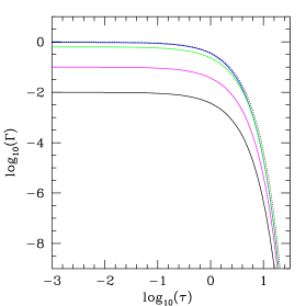
Figure 1: Photoionization rate from Eq. (2) evaluated based on the optical depth, $\tau$, up to the cell (dotted line) compared to the photon-conserving photoionization rates from Eq. (6) for $\Delta\tau=0.1,1,10,$ and 100 (solid lines; top to bottom) vs. optical depth $\tau$ from the source to the cell. We normalized the rates to 1 for $\tau\ll 1$ and $\Delta\tau\ll 1$, assuming $r\gg\Delta r$ and gray opacities (i.e. $\sigma_{\nu}=$ constant).

In Figure 1 we illustrate the difference between the local photoionization rate, $\Gamma_{\rm local}(r)$ from Eq. (2) evaluated at the entrance point of a cell and the photon-conserving photoionization rate, $\Gamma$, from Eq. (6) over the finite cell. We plot $\Gamma$ for optical depths per cell $\Delta\tau=0.1,1,10,$ and 100, and $\Gamma_{\rm local}(r)$ (which is independent of $\Delta\tau$) vs. the optical depth up to the cell, $\tau$. All rates are calculated in gray-opacity approximation (photoionization cross-section independent of frequency). We clearly see that, as expected, the local photoionization rate agrees well with the photon-conserving rates only for optically-thin cells ($\Delta\tau<0.1$), in which case the two curves are barely distinguishable. However, the two rates start to differ significantly even for moderately optically-thick cells ($\Delta\tau\sim 1$) and are completely different for highly optically-thick cells ($\Delta\tau>10$). In practice, the main differences when using photon-conserving finite-differenced rates would arise for moderately optically-thick cells for which the optical depth from the source $\tau$ is low to moderate. For a cell which is either shielded or self-shielded (i.e. either $\tau$ or $\Delta\tau$ is large), the photoionization rate would be very low, and hence even incorrect photoionization rates would have no appreciable impact on the ionized fraction.

Another way to think of the photon-conserving photoionization rate in Eq. (6) is to notice that for thin shell, $\Delta r\ll r$, and gray opacity ($\sigma_{\nu}=$constant) we have

$$\Gamma=\frac{\Gamma_{\rm local}(r)-\Gamma_{\rm local}(r+\Delta r)}{\Delta\tau}.$$ (7)

This shows that the fractional error introduced by using Eq. (2) evaluated at the shell inner edge radius to give the ionization rate for all atoms in the shell, is given by $[\Gamma_{\rm local}(r)-\Gamma_{\rm local}(r+\Delta r)]/\Gamma=\Delta\tau$ and hence grows as $\Delta\tau$ grows. This again demonstrates that $\Gamma_{\rm local}$ evaluated at the inner cell boundary is a good approximation to the finite-cell photon-conserving rate only for optically-thin cells.

2.2 Temporal discretization

When using the photoionization rate $\Gamma$ to integrate the ionization equations over a time step $\Delta t$, one normally assumes it to be constant during this time step. However, since the ionizations and recombinations in the cell will change the density of neutral hydrogen, the optical depths $\tau_{\nu}$ and $\Delta\tau_{\nu}$ will also change. The usual solution is to take $\Delta t$ which is small enough so the optical depths do not change appreciably over one step. For fast moving I-fronts this demands very short time steps. Various authors use different criteria in determining what the time step should be: a fraction of the photon travel time over a cell $\Delta r/c$ (Abel et al. 1999), several times the ionization time $\Gamma^{-1}$ (Bolton et al. 2004), a small fraction of the timescale of change of the H I fraction, $n_{\rm HI}/({\rm d}n_{\rm HI}/{\rm d}t)$, (which sets the speed of the ionization front, Shapiro et al. 2004). Such small time steps make for expensive calculations if high accuracy is to be achieved.

Since the above rate $\Gamma$ is really a time-averaged rate (we only know what went in and what came out of the cell, not what happened in detail within the cell), a time-averaged value for $\Delta\tau_{\nu}$ can be expected to relax the constraint on the time step. We illustrate this with the following simplified model. Consider an infinitely-thin parcel of hydrogen gas of number density $n$ illuminated by a time-varying photon flux $F_{\nu}(t)$. Neglecting for the moment the effect of recombinations and collisional ionizations, the ionization rate equation can be written as

$$\frac{{\rm d}y_{\rm HI}}{{\rm d}t}=-\Gamma y_{\rm HI}.$$ (8)

where $y_{\rm HI}$ is the neutral fraction of hydrogen. If we define a time-averaged photoionization rate, $\langle\Gamma\rangle$, as

$$\langle\Gamma\rangle=\frac{1}{\Delta t}\int_{t}^{t+\Delta t}\Gamma(t^{\prime}){\rm d}t^{\prime},$$ (9)

then the solution to Eq. (8) is identical to that of

$$\frac{{\rm d}y_{\rm HI}}{{\rm d}t}=-\langle\Gamma\rangle y_{\rm HI}.$$ (10)

This shows that, if only photoionizations contribute to the rate equation, it is correct to treat the ionization rate as a constant over the time step, no matter how large $\Delta t$ is, as long as we take its value to be the time-average of $\Gamma$ over $\Delta t$. If recombinations and collisional ionizations are taken into account, then this is not necessarily true since photoionizations that happen early in the time interval are more likely to be canceled by recombinations than those that happen later. However, as we shall show, using the time-averaged flux only introduces appreciable deviations from photon-conservation when the time step becomes comparable to the recombination time of the cell, and even in such cases the approximation holds fairly well.

Solving for the ionization fractions is in itself not entirely trivial since we are dealing with stiff partial differential equations. Still considering only hydrogen, then the evolution of the ionized fraction $x\equiv 1-y_{\rm HI}$ can be written as

$${{\rm d}x\over{\rm d}t}=(1-x)(\Gamma+n_{\rm e}C_{H})-xn_{\rm e}\alpha_{H}\,,$$ (11)

where $n_{\rm e}$ is the electron density (itself dependent on the ionization fraction $x$) and $C_{H}$ and $\alpha_{H}$ are, respectively, the (temperature-dependent) collisional ionization and recombination coefficients for hydrogen. In this paper we assume the On-The-Spot (OTS) approximation (i.e. that the recombinations to the ground state are locally reabsorbed), in which case the recombination coefficient $\alpha_{H}$ is equal to $\alpha_{B}=2.59\times 10^{-13}(T/10^{4}\,K)^{-0.7}$ cm³ s^-1, the Case B recombination coefficient for hydrogen at gas temperature $T$.

If one takes $\Gamma$, $n_{\rm e}$, $C_{H}$ and $\alpha_{H}$ to be constant, this equation has an analytical solution

$$x(t)=x_{\rm eq}+(x_{0}-x_{\rm eq})e^{-t/t_{\rm i}}\,,$$ (12)

with

$$t_{\rm i}=1/(\Gamma+n_{\rm e}C_{H}+n_{\rm e}\alpha_{H})\,,$$ (13)

and

$$x_{\rm eq}={\Gamma+n_{\rm e}C_{H}\over\Gamma+n_{\rm e}C_{H}+n_{\rm e}\alpha_{H}}\,.$$ (14)

Schmidt-Voigt & Koeppen (1987) suggested using this solution, and iterating for the electron density. The approach can be expanded to include other atomic species such as helium and metals. This method was successfully used by e.g. Frank & Mellema (1994); Raga et al. (1997); Mellema et al. (1998); Shapiro et al. (2004); Iliev et al. (2005d), to name a few examples. In order not to have to repeatedly calculate the integrals over the spectrum, they are tabulated as function of the optical depth at $\nu_{\rm th}$, the ionization threshold of hydrogen, which, together with the spectral shape completely determines these integrals. We refer the reader to the above papers for further details on this method for solving the non-equilibrium chemistry equations.

In the current context this approach for following the chemistry evolution equations is particularly appealing since it provides us with an analytical expression for the time-averaged ionization fraction

$$\langle x\rangle=x_{\rm eq}+(x_{0}-x_{\rm eq})(1-e^{-\Delta t/t_{\rm i}}){t_{\rm i}\over\Delta t}\,,$$ (15)

which can in turn be used to find the time-averaged optical depth of the cell $\langle\Delta\tau\rangle$, as follows:

$$\langle\Delta\tau_{\nu}\rangle=(1-\langle x\rangle)n_{H}\sigma_{\nu}\Delta r,$$ (16)

where $\langle x\rangle$ is given by Eq. (15).

Figure 2: Flow chart of our method for a given computational cell.

In order to remain self-consistent, the value of the $\langle x\rangle$ should then be used to modify $\Gamma$ by changing both the optical depth and the neutral density:

$$\Gamma=\int_{\nu_{\rm th}}^{\infty}{L_{\nu}e^{-\langle\tau_{\nu}\rangle}\over h\nu}{1-e^{-\langle\Delta\tau_{\nu}\rangle}\over\langle n_{\rm HI}\rangle V_{\rm shell}}{\rm d}\nu\,,$$ (17)

which leads to an iterative process. Furthermore, since $n_{\rm e}$ plays a role similar to $\Gamma$, we use its time-averaged value $\langle n_{\rm e}\rangle$ when evaluating the ionization Eq. (11). The optical depth between the source and the cell edge $\tau_{\nu}$ is replaced by its time-averaged value, by adding, in causal order, all the time-averaged $\langle\Delta\tau_{\nu}\rangle$ of the cells lying between the source and the cell under consideration. This total optical depth (evaluated at the ionizing threshold of hydrogen, $\tau_{0}=\tau_{\nu=\nu_{\rm th}}$), is used to look up the values of the integral

$$\Gamma^{\prime}(\tau_{0})\equiv\int_{\nu_{\rm th}}^{\infty}\frac{L_{\nu}e^{-\langle\tau_{\nu}\rangle}}{h\nu\langle n_{\rm HI}\rangle V_{\rm shell}}{\rm d}\nu\,,$$ (18)

in pre-calculated tables. Then the photoionization rate in Eq. (17) is given by $\Gamma=\Gamma^{\prime}(\tau_{0})-\Gamma^{\prime}(\tau_{0}+\Delta\tau_{0})$, where $\Delta\tau_{0}=\Delta\tau_{\nu=\nu_{\rm th}}$.

In practice, the iteration for finding the ionization state of a given cell proceeds as follows (see flowchart in Figure 2):

1. Initialize the mean ionization state to the initial values (given by the previous time step or the initial conditions).

2. Find the column density between the source and the cell

3. Iterate until convergence in the neutral fraction(s):

   • Calculate time-averaged column density of the cell [Eq. (16)].

   • Calculate the photoionization rate $\Gamma$ [Eq. (17)].

   • Calculate the mean electron number density, $\langle n_{e}\rangle$, based on the current mean ionization state.

   • Calculate new and mean ionization states [Eqs. (11)-(15)].

   • Check for convergence.

To illustrate the ability of our method to obtain the correct result with a small number of time steps, we consider the problem of formation and evolution of an H II region around a single source in an uniform, initially-neutral density distribution, which has an exact analytical solution (this is Test 1 in § 5 below, see there for details on the numerical parameters and the setup). We use a one-dimensional grid of 256 cells, gray opacities and uniform time steps. The optical depth per cell when it is fully-neutral is $\tau_{\rm cell}=11.5$. We solve this problem two ways, using the time-averaged photoionization rate in Eq. (17) with 100 time steps, and using the non-time-averaged rates in Eq. (6) evaluated at the beginning of each time step using $10^{2},10^{3},10^{4}$ and $10^{5}$ uniform time steps. Results are shown in Figure 3. The time-averaged photoionization rates solution is essentially indistinguishable from the analytical result, with errors much smaller than 1%. To achieve a similar precision using the non-time-averaged photoionization rates we need up to $\sim 10^{5}$ time steps, or a factor of a 1000 more than in our method. The method with $\sim 10^{4}$ time steps and no time-averaging still gives an acceptable, but clearly inferior solution, which is off by a few per cent from the analytical result. Using any smaller number of time steps and no time-averaging leads to a completely incorrect evolution, whereby the I-front initially propagates much more slowly than it should have, and producing a much smaller H II region. It should be noted that ultimately even in those cases the correct Strömgren sphere is reached, but only at much later times.

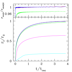
Figure 3: Spherical I-front for point source in uniform gas: (a)(bottom panel) radius (in units of the Strömgren radius $r_{S}$) vs. time (in units of recombination time $t_{\rm rec}$). Time-averaged photon-conserving photoionization rates from Eq. (17) for $10^{2}$ time steps (top line) and the non-time-averaged (but otherwise also photon-conserving) rates from Eq. (6) evaluated at the beginning of each time step, for $10^{2},10^{3},10^{4}$ and $10^{5}$ time steps (bottom to top lines). Note that the top curves (time-averaged and $10^{5}$ step non-time-averaged) are almost indistinguishable. (top panel) Ratios of the numerical solutions over the analytical one, $r_{\rm num}/r_{\rm analyt}$. Top lines, largely indistinguishable, are the time-averaged solution and non-time-averaged solution for $10^{5}$ time steps, bottom line is the non-time-averaged solution for $10^{4}$ time steps.

The reason why the method without time-averaging of the optical depth would need many more time steps is that it requires the time step, $\Delta t$, to be shorter (ideally much shorter) than the cell-crossing time, $t_{\rm cross}=\Delta x_{\rm cell}/v_{I}$, (i.e. that the I-front does not cross more than one cell per time step). When the I-front is very fast this condition demands very short time steps. In particular problems, where the I-fronts either propagate more slowly, or the fast-propagation phase is short-lasting, utilizing such short time steps could be feasible (see e.g. Shapiro et al. 2004), although still computationally-expensive. In more general situations, e.g. a cosmological density field, I-fronts often propagate very fast at least somewhere in the computational domain. In such problems using time-averaging of the optical depths is indispensable for this type of radiative transfer method.

3 Ray tracing

The method described in § 2 is one-dimensional, or in other words, along a ray. In order to use it in three spatial dimensions, we need to trace rays across the computational domain. Different ray-tracing methods exist and could be combined with our method, as long as the rays are traversed in a causal order away from the source. Here we use a method called ’short characteristics’, in which the rays for each point are constructed from previously calculated neighboring points, instead of casting independent rays to each cell (’long characteristics’). This is the approach used by Raga et al. (1999) and Lim & Mellema (2003), with minor modifications. This method scales with the number of cells in the computational mesh. We describe our method in detail in Appendix A.

Figure 4: Flow chart for the case of multiple sources.

4 Treatment of Multiple Sources

When multiple sources of ionizing radiation are present, we start by calculating the optical depths from each source outwards by casting rays to each cell and using the method of short characteristics, as described in Appendix A. As we loop through the sources (in random order) we add the contribution of each source to the total photoionization rate, and we save the solution for the (time-averaged) neutral fractions. The latter implicitly communicates the presence of other sources to the current source. After having treated all sources we apply the total photoionization rate to the whole grid, this time without tracing any rays. This procedure is repeated until the final neutral fraction satisfies our convergence criterion. Note that in the multiple source case we do not test for convergence when treating individual sources, but do so only at the end, when we apply the total photoionization rates from all sources. Figure 4 shows the above procedure in the form of a flow chart.

Since ray-tracing is done for each individual source, the method roughly scales with the number of sources times the typical number of iterations needed for convergence. The latter number depends on the density field and the amount of overlap between the H II regions, so it is hard to give a general number. Experience shows it to be typically less than 10.

Source numbers, positions, luminosities, starting times and lifetimes could be read in from a file or determined internally by the code. Currently all sources have the same spectrum, but within the framework of our method it is easy to implement several types of sources (e.g.  Pop. II and III starbursts, QSO’s) by creating and using separate lookup tables for the photoionization rates for each source type.

5 Tests

5.1 Expansion of H II regions about a single source

We first consider the simplest case of H II region expansion, namely around a single source of ionizing radiation in a fixed density field. Consider a source emitting $\dot{N}_{\gamma}$ ionizing photons per unit time igniting in an initially-neutral medium consisting of pure hydrogen with number density $n_{H}$. The source propagates an I-front into the neutral gas. The I-front propagation speed is determined by the balance at the I-front of the incoming flux of ionizing photons and the flux of neutral atoms flowing into the I-front and getting ionized. Assuming for simplicity that the I-front is “sharp”, i.e. the width of the neutral-ionized transition region is small compared to the I-front radius, then this balance is expressed by the I-front jump condition:

$$n_{H}\frac{{\rm d}r_{I}}{{\rm d}t}=F,$$ (19)

where $n_{H}$ is the number density of hydrogen atoms and $F$ is the flux of ionizing photons at the I-front. $F$ is equal to the photon output of the source per unit time, $\dot{N}_{\gamma}$, minus the photons lost to recombinations in the already ionized volume, $V_{I}=4\pi r_{I}^{3}/3$:

$$F=\frac{1}{4\pi r_{I}^{2}}\left(\dot{N}_{\gamma}-\int_{V_{I}}n_{H}^{2}C\alpha_{B}dV\right),$$ (20)

where $C\equiv\langle n^{2}\rangle/\langle n\rangle^{2}$ is the volume-averaged clumping factor of the gas (for a uniform gas $C=1$), which increases the recombination rate of the ionized gas. Combining Eqs. (19) and (20), we obtain

$$n_{H}\frac{dV_{I}}{{\rm d}t}={\dot{N}_{\gamma}-\int_{V_{I}}n_{H}^{2}C\alpha_{B}dV}$$ (21)

The width of an I-front is determined by the mean free path of the ionizing photons at the front. The assumption of “sharp” I-front is generally well-justified for soft ionizing spectra, but not necessarily for harder spectra, in which case the transition from neutral to ionized gas at the front could get fairly wide (see Shapiro et al. 2004, for further discussion and specific examples).

We performed four tests of single-source I-front propagation in several density fields relevant to astrophysics, which are listed in Table 1 and described in more detail below. In § 5.1.1 and § 5.1.2 we discuss the results in 1D spherical symmetry, and 3D, respectively, with the temperature kept fixed at $10^{4}$ K. For simplicity, we assume that the gas consists of pure hydrogen. While here we consider only the case of a pure hydrogen gas, our non-equilibrium chemistry solver can also easily accommodate multiple species (see e.g. Mellema et al. 1998; Shapiro et al. 2004). We also assume a gray opacity. In this limit the photoionization rate from Eq. (17) becomes proportional to the number of ionizing photons produced by the ionizing source per unit time:

$$\Gamma \propto \dot{N}_{\gamma}=\int_{\nu_{\rm th}}^{\infty}\frac{L_{\nu}}{h\nu}d\nu$$ (22)

In this simple setting there are exact analytical solutions for both the I-front position and velocity for all density fields we consider in our tests. To our knowledge, some of these solutions are derived here for the first time.

In all tests the computational domain size was chosen so that it is only slightly larger than the final H II region size in order to keep the resolution roughly similar between the different tests. The source position for the 1D, spherical symmetry tests is at the origin, $r=0$, while for the 3D tests the source is in the center of the grid. We run each test four times in 1D and four times in 3D, all possible combinations of two different spatial resolutions (“coarse” one with 16 cells, i.e. $\Delta x_{\rm cell}=x_{\rm box}/16$, and “fine” one with 128 cells in 1D, as well as the corresponding $32^{3}$ and $256^{3}$ cells in 3D), and two different choices of time steps, $\Delta t_{\rm coarse}=t_{\rm evol}/10$ and $\Delta t_{\rm fine}=t_{\rm evol}/100$, where $t_{\rm evol}$ is the total time for which we follow the I-front. For our coarse-resolution runs we chose these very low spatial and time resolutions in order to demonstrate the conservative properties of our method. There are many problems where such low resolutions are expected, e.g. during reionization when we try to follow the initial evolution of multiple H II regions in a large simulation volume, so it is important to establish how reliable are the simulation results in such situations. Our “fine” resolution runs also employ relatively modest resolutions in both time and space, which enables us to easily run the 1D and the 3D simulation results at equivalent resolutions in order to directly compare the results from the two. In all tests the parameters we picked are such that the individual cells start very optically-thick (see Table 1), so as to thoroughly test our code in such most demanding situations.

We define the I-front position to be at the point where the gas is 50% neutral. Note that if the I-front width (which is typically 10-20 photon mean-free-paths, and is thus dependent on the type of ionizing spectrum and the spectrum hardening ahead of the I-front) is unresolved (the front is “sharp”), then the exact value of the neutral fraction used to define the I-front position is irrelevant. However, when the I-front structure is resolved (the front is “thick”), then its position (but not its velocity) depends on the neutral fraction at which we define it. Therefore, in such cases the I-front position obtained numerically could be offset from the position given by the analytical solutions, which all assume “sharp” I-fronts for simplicity. Inside a cell the I-front position is found by linear interpolation. The numerical value for the I-front velocity, $v_{I}$, was obtained by simple finite-differencing of its position and the time, according to

$$v_{i}(t_{i,ave})=\frac{r_{i}-r_{i-1}}{t_{i}-t_{i-1}},$$ (23)

where $t_{i,ave}=(t_{i}+t_{i-1})/2$. Whenever the time for the I-front to cross a cell is larger than the time step, the average speed of the front over a single time step is numerically poorly defined by Eq. (23). In that case, the speed was evaluated over a larger interval of time, comparable or greater than the cell-crossing time.

Table 1: Parameters of the test problems described in the text. The box sizes listed are for the 3D tests. For the corresponding 1D tests we used a box size which was one-half of the values listed. $\tau_{0,cell,min}$ and $\tau_{0,cell,max}$ are the minimum and maximum optical depth per cell (when neutral) at the Lyman limit of hydrogen at the corresponding resolution (lr=low resolution run, hr=high-resolution run).

Test	1	2	3	4
$\dot{N}_{\gamma}$(s-1)	$10^{54}$	$10^{51}$	$10^{51}$	$10^{54}$
$n_{\rm HI}$ (cm-3)	$1.87\times 10^{-4}$	0.015$\left(\frac{5~{}\mathrm{kpc}}{r}\right)$	$3.2\left(\frac{91.5~{}\mathrm{pc}}{r}\right)^{2}$	$1.87\times 10^{-4}(1+z)_{10}^{3}$
$C$	5	1	1	5
$t_{\rm evol}$ (Myr)	$500$	15	1	$500$
$x_{\rm box}$ (cm)	$5\times 10^{24}$	$1.4\times 10^{22}$	$6\times 10^{21}$	$7\times 10^{25}$ (comov.)
$t_{\rm rec}$ (Myr)	$130$	$8.2\left(\frac{r}{5\,\rm kpc}\right)$	$0.04\left(\frac{r}{91.5\,\rm pc}\right)^{2}$	$130(1+z)_{10}^{-3}$
$r_{S}$ (kpc)	$563$	$1.86$	…	…
$t_{\rm evol}/t_{\rm rec}$	3.85	$1.84\left(\frac{r}{5\,\rm kpc}\right)^{-1}$	$26\left(\frac{r}{91.5\,\rm pc}\right)^{-2}$	$3.85(1+z)_{10}^{3}$
$\tau_{0,cell,min}$,lr	184	91	34	50
$\tau_{0,cell,min}$,hr	23	11	4	6
$\tau_{0,cell,max}$,lr	184	2200	3800	184
$\tau_{0,cell,max}$,hr	23	2200	470	23

Test 1 involves the simplest situation, an I-front propagating in a uniform, constant gas density $n_{H}$ with a constant clumping factor $C$. There is a well-known analytical solution for the expansion of such an I-front, which is determined by two parameters, the Strömgren radius $r_{\rm S}$ and the recombination time $t_{\rm rec}$ (see e.g. Dopita & Sutherland 2003), which are defined as

$$r_{\rm S}=\left[{3\dot{N}_{\gamma}\over 4\pi\alpha_{B}(T)Cn_{\rm H}^{2}}\right]^{1/3}\,,$$ (24)

and

$$t_{\rm rec}=\left[C\alpha_{B}(T)n_{H}\right]^{-1}\,.$$ (25)

The analytical expressions for the I-front position, $r_{I}$ and velocity, $\rm v_{I}$, as a function of time are then

$$r_{I} = r_{\rm S}\left[1-\exp(-t/t_{\rm rec})\right]^{1/3}\,.$$ (26)

$$\rm v_{I} = \frac{r_{\rm S}}{3t_{\rm rec}}\frac{\exp{(-t/t_{\rm rec})}}{\left[1-\exp(-t/t_{\rm rec})\right]^{2/3}}\,,$$ (27)

i.e. the H II region reaches a finite radius, $r_{S}$, and zero velocity at $t\rightarrow\infty$ (in practice, after a few recombination times), at which point the recombinations in the ionized volume balance the new photons arriving from the source. In physical units we choose typical values for cosmological I-fronts propagating during reionization, with the gas density equal to the mean density of the universe at redshift $z=9$ and a source with ionizing photon production rate $\dot{N}_{ph}=10^{54}\,\rm s^{-1}$ (Table 1).

In Test 2 we study the propagation of an I-front from a source in the center of a singular, decreasing density profile $n_{H}=n_{0}(r_{0}/r)$, where $n_{0}=0.015\,\rm cm^{-3}$ is the gas number density at the characteristic radius $r_{0}=5\,\rm kpc$. This test is related to the problem of an I-front propagating outward from a source in the center of a galactic halo with a Navarro, Frenk & White profile (Navarro et al. 1997) (assuming the gas follows the dark matter density profile). For this density profile Eq. (21) reduces to

$$\frac{{\rm d}r_{I}}{{\rm d}t}=\frac{L}{r_{I}}-K,$$ (28)

where we defined $L\equiv{\dot{N}_{\gamma}}/{(4\pi n_{0}r_{0})}$, $K\equiv{n_{0}r_{0}C\alpha_{B}}=r_{0}/t_{\rm rec,0}$, where $t_{\rm rec,0}\equiv(n_{0}C\alpha_{B})^{-1}$ is the recombination time at the characteristic density $n_{0}$. Eq. (28) has an analytical solution, which for initial condition $r(0)=0$ is given by

$$r_{I}(t)=r_{S}\left\{1+{\rm LambertW}\left[-\exp\left(-\frac{r_{0}t}{r_{S}t_{\rm rec,0}}-1\right)\right]\right\},$$ (29)

where $r_{S}=L/K$ is the Strömgren radius for this test and ${\rm LambertW}(x)$ is the solution of the algebraic equation $y(x)e^{y(x)}=x$, which can be calculated e.g. using readily available public software.

In Test 3 we follow the propagation of an I-front in a density profile $n_{H}=n_{0}(r_{0}/r)^{2}$, with a flat core of gas number density $n_{0}$ and radius $r_{0}$. This density profile is steeper than the one we consider in Test 2, and the H II region evolution is qualitatively different, as we show below (see also Franco et al. 1990; Shapiro et al. 2005b, for detailed discussion of I-front propagation in power-law density profiles). This test, with the dimensional parameters we have chosen, $n_{0}=3.2\,\rm cm^{-3}$ and $r_{0}=91.5\,\rm pc$, (Table 1) resembles the problem of inside-out ionization of a dwarf galaxy formed at redshift $z=9$ by an ionizing source at its center. In this case Eq. (21) reduces to

$$\frac{{\rm d}r_{I}}{{\rm d}t}=L+\frac{K}{r_{I}},$$ (30)

where we defined

$$L=v_{\rm lim}\equiv\frac{\dot{N}_{\gamma}}{4\pi n_{0}r_{0}^{2}}-\frac{4}{3}n_{0}r_{0}C\alpha_{B},$$ (31)

which physically is the terminal velocity $v_{\rm lim}$ of the I-front for $r\rightarrow\infty$, and $K\equiv n_{0}r_{0}^{2}C\alpha_{B}=r_{0}^{2}/t_{\rm rec,core}$. Assuming that $\dot{N}_{\gamma}>4\pi r_{0}^{3}n_{0}^{2}C\alpha_{B}/3$ i.e. source is strong enough to ionize more than just the core, it is clear that $v_{I}>0$ for all radii and thus the I-front will never stop, eventually reaching the constant terminal velocity $v_{\rm lim}$. Equation (30) for arbitrary values of the parameters $K$ and $L$ has a complex analytical solution for the initial condition $r(0)>r_{0}$. However, one particularly simple solution is obtained when $L=0$, i.e. $\dot{N}_{\gamma}=16\pi r_{0}^{3}n_{0}^{2}C\alpha_{B}/3$, and $r(0)=r_{0}$, in which case the radius of the I-front is given by

$$r_{I}=r_{0}(1+2t/t_{\rm rec,core})^{1/2}.$$ (32)

This is the case we will use in our Test 3. In calculating the column densities for this test we use the weightings in Eq. (43) with $\tau_{0}=\epsilon>0$, where $\epsilon\ll 1$.

Finally, our Test 4 is the same as Test 1, but for a cosmological I-front propagating in a uniform-density medium with a density equal to the time-evolving mean background density of the universe. The ionizing source is switched on at redshift $z=9$. The I-front evolution of cosmological I-front in an IGM with mean volume-averaged clumping factor $C$ has an exact analytical solution (Shapiro & Giroux 1987), given by

$$y(x)={\lambda}e^{\lambda/x}\left[xEi(2,{\lambda}/{x})-Ei(2,\lambda)\right].$$ (33)

Here $y\equiv[r_{I,c}(t)/r_{S,i}]^{3}$, $r_{I,c}=r_{I}(1+z)$ is the comoving radius of the I-front at time $t^{\prime}=t_{i}+t$, $r_{S,i}=[3\dot{N}_{\gamma}/(C\alpha_{B}(n_{H,c})^{2})]^{1/3}$ is the initial Strömgren radius, $n_{\rm H,c}$ is the mean comoving density of hydrogen (defined at epoch of source turn-on, i.e. the scale factor is normalized $a_{i}=1$),

$$\lambda\equiv\frac{t_{i}}{t_{\rm rec,i}}=t_{i}C\alpha_{B}n_{H,c},$$ (34)

is the ratio of recombination time at present to the age of the universe when the source turned on, and $Ei(2,x)\equiv\int_{1}^{\infty}\frac{e^{-xt}}{t^{2}}{\rm d}t$ is the Exponential integral of second order. Note that the exponent in the analytical solution in Eq. (33), $e^{\lambda t_{i}/t}$, is generally very large, which could easily lead to numerical overflow problems. There is a similar exponent, but with negative sign, in the Exponential integrals and it is therefore better to numerically evaluate them together, as $e^{\lambda t_{i}/t}Ei(2,\eta\frac{t_{i}}{t})$, rather than separately.

5.1.1 1D Ionization Fronts

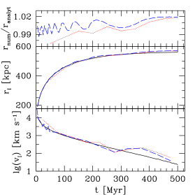
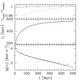
Figure 5: Ionization front evolution for Test 1 (H II region expansion in an uniform gas) in 1D spherical symmetry, using coarse grid (left panels) and fine grid (right panels). Shown are the analytical solution (solid, black), and the numerical solutions for $\Delta t_{\rm coarse}$ (dotted, red) and $\Delta t_{\rm fine}$ (dashed, blue) for the I-front position (middle panels), ratio of the numerical to the exact analytical position (top panels) and the I-front velocity (bottom panels).

Figure 5 shows our results for Test 1 (constant density). The numerical results match the exact analytical solution quite well, even at very low spatial and temporal resolutions. The I-front position is never off by more than a fraction of a cell size at the corresponding spatial resolution. The only exception is the low temporal, but high spatial resolution case where the H II region size is initially underestimated by a few per cent (or $\sim 1.25$ cell-sizes). However, even in this case the agreement quickly improves and the final Strömgren radius is excellently reproduced. The numerical I-front velocity is also in excellent agreement with the analytical solution, regardless of the time- or spatial resolution, although the coarse spatial resolution runs tend to overestimate the I-front speed slightly when the I-front slows down below $v_{I}\approx 100\,\rm km\,s^{-1}$. This could be expected, since the I-front cell-crossing time for this velocity is $t_{\rm cross}\approx 500$ Myr, i.e. the I-front has essentially stalled and remains inside a single cell, making the velocity estimate unreliable. This is confirmed by our higher spacial resolution runs shown in Figure 5 (right) in which case the cell-crossing time for the same I-front velocity is 8 times shorter and hence the velocity is correctly reproduced down to few tens of $\rm km\,s^{-1}$.

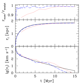
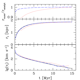
Figure 6: I-front evolution for Test 2 (H II region expansion in $r^{-1}$ density profile) in 1D spherical symmetry. Same notation as in Fig. 5.

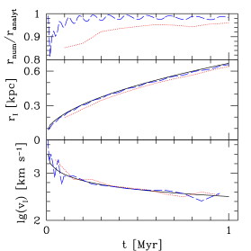
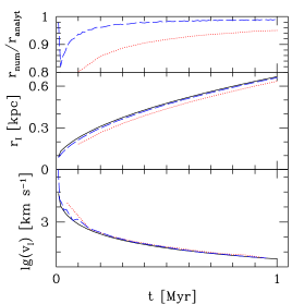
Figure 7: I-front evolution for Test 3 (H II region expansion in $r^{-2}$ density profile) in 1D spherical symmetry. Same notation as in Fig. 5.

In summary, for this test, the good temporal resolution is more important in achieving good agreement with the analytical solution than is high spatial resolution, although the results from our numerical method are quite acceptable in all cases.

The reason for this behavior is that for time steps of order of the recombination time, our method overestimates the number of recombinations. In this test problem this happens when, within one time step, the H II region almost reaches its Strömgren sphere and the I-front essentially stalls. In this case, some cells near the front remain neutral for a large part of the time step. Using the time-averaged electron density in this case overestimates the number of recombinations. A better result is obtained if the time step, $\Delta t$ is significantly shorter than the recombination time, $t_{\rm rec}$, while here $\Delta t_{\rm coarse}=50\,\rm Myr=0.4t_{\rm rec}$.

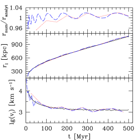
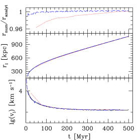
Figure 8: I-front evolution for Test 4 (cosmological H II region expansion) in 1D spherical symmetry. Same notation as in Fig. 5.

Our results for Test 2 ($1/r$ density) are shown in Figure 6. In this case the density profile is singular, and hence the evolution is dominated by recombinations from the start, rather than just at late times as was in Test 1. The H II region reaches the correct Strömgren radius, with errors $\sim 1\%$ in all cases regardless of the resolution, but once again the early evolution of the H II region is much better followed (generally within 1-2% or better) in the runs with higher temporal resolution. However, even for very poor time resolution the I-front position is correct within $\sim 10\%$, and to better than 4% after the first few time steps. The reason for this small initial discrepancy is that the recombination time in the inner, high-density cells is very short, shorter than (or at most of order) $\Delta t_{\rm coarse}=1.5$ Myr, and hence the numerical I-front initially propagates slightly slower than it should. Nonetheless, thereafter the I-front velocity is correctly reproduced in all cases up to the Strömgren sphere.

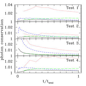
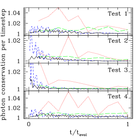
Figure 9: Photon conservation for Tests 1-4 in 1D. Cases plotted are: 16 cells, 10 time steps (red, dotted), 16 cells, 100 time steps (blue, short-dashed), 128 cells, 10 time steps (green, long-dashed), 128 cells, 100 time steps (black, solid).

Test 3 ($1/r^{2}$ density) proved most difficult for our numerical method to follow at low temporal resolutions (Figure 7). The H II region is smaller than the exact, analytical one by 5-10% percent (and up to 20% at the very beginning). Within one such relatively long time step ($\Delta t_{\rm coarse}=0.1$ Myr) the I-front crosses the density profile core and advances significantly down the steep density gradient. The recombination time in the core is $t_{\rm rec,core}=0.04$ Myr and $\Delta t_{\rm coarse}=2.5t_{\rm rec,core}$. Our time-averaging procedure slightly overestimates the mean optical depth over the time step in such conditions. Interestingly, the I-front exact analytical velocity is nevertheless perfectly reproduced. Thus for coarse time steps the I-front propagates at the correct speed, but with slightly offset position. In the high temporal resolution cases the analytical I-front radius is matched to better than a few percent after the first few steps, regardless of the spatial resolution employed.

Test 4 (expanding universe) resulted in excellent agreement between our numerical solution and the exact one, for all spatial and temporal resolutions (Figure 8). This was in fact expected, since in this case the recombination time is always longer than even our coarse time step, i.e. $t_{\rm rec}/\Delta t_{\rm coarse}=2.6/(1+z)_{10}^{3}$, especially at later times as the background expands with the Hubble flow. We note that, as a consequence of this continuous decrease of the gas density, the Strömgren sphere is never reached and the I-front velocity remains very fast at all times, always above $10^{3}\rm km\,s^{-1}$, i.e. the I-front is of fast, R-type. This is a generic property of global cosmological I-fronts, as was first shown by Shapiro & Giroux (1987).

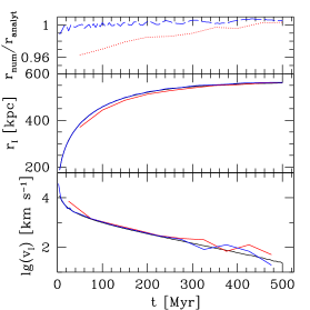
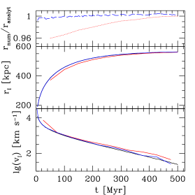
Figure 10: I-front evolution for Test 1 (H II region expansion in an uniform gas) in 3D, using $32^{3}$ cells (left panels) and $256^{3}$ cells (right panels), otherwise same notation as in Fig. 5.

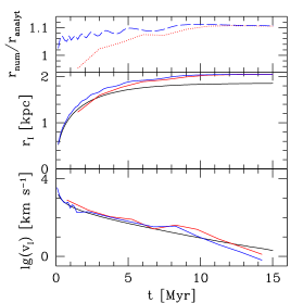
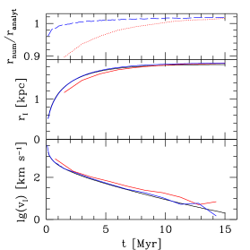
Figure 11: I-front evolution for Test 2 (H II region expansion in $r^{-1}$ density profile) in 3D. Same notation as in Fig. 10.

Finally, in Figure 9 we show the photon conservation numbers, which we define as the ratio of the total of all new ionizations and recombinations divided by the number of photons provided by the ionizing source per time step (right), or integrated over time (left) for Tests 1-4 in 1D spherical symmetry. We see that, even at the coarsest space- and time-discretizations, photons are generally conserved to within a few per cent. When either the spatial- or the time-resolution is not the coarse one the photon conservation of our method is generally better than 1%.

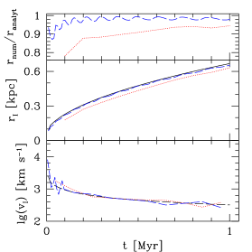
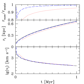
Figure 12: I-front evolution for Test 3 (H II region expansion in $r^{-2}$ density profile) in 3D. Same notation as in Fig. 10.

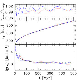
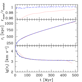
Figure 13: Ionization front evolution for Test 4 (cosmological H II region expansion) in 3D. Same notation as in Fig. 10.

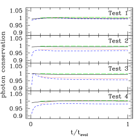
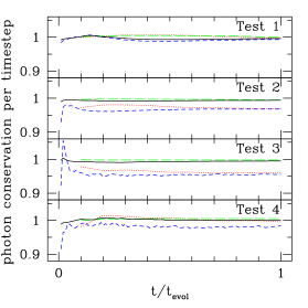
Figure 14: Photon conservation for Tests 1-4 in 3D. Cases plotted are: $32^{3}$ cells, 10 time steps (red, dotted), $32^{3}$ cells, 100 time steps (blue, short-dashed), $256^{3}$ cells, 10 time steps (green, long-dashed), $256^{3}$ cells, 100 time steps (black, solid).

5.1.2 3D Ionization Fronts

Figure 15: I-front evolution. Shown is the 0.5 ionization level contour in time-sequence from $t=0.1t_{\rm evol}$ to $t=t_{\rm evol}$, every $0.1t_{\rm evol}$ for Tests 1-4, as labeled. All plots are for the case with coarsest-resolution in both space and time. On all occasions the I-front remains spherical at all times except for slight non-sphericity in Test 3 ($1/r$ density). In all higher-resolution cases the I-front remains perfectly spherical at all times.

For the 3D tests we use the same approach as in § 5.1.1, i.e. constant temperature at $T=10^{4}$ K and gray opacities. The resolutions used are a coarse one at $32^{3}$ cells and a fine one at $256^{3}$ cells. We placed the source in the center of the grid. Hence, the radial profiles are calculated at radial resolution of 128 and 16 cells, respectively, and are thus directly comparable to the 1D results in § 5.1.1. Again, for each case we use two temporal resolutions, $\Delta t_{\rm coarse}=t_{\rm evol}/10$ and $\Delta t_{\rm fine}=t_{\rm evol}/100$. Results are shown in Figs. 10-14. The radial cuts are along the positive $x$-axis. The results are largely identical to the corresponding ones in 1D spherical symmetry. The numerical solution slightly overestimates the initial I-front velocity for low temporal resolution cases in Tests 1 (uniform density) and 2 ($1/r$ density). The final Strömgren spheres in the same Tests 1 and 2 have the correct sizes, to within few per cent, except for low spatial resolution runs of Test 2, where it is off by about 10%, or slightly more than 1 cell size. Once again the low temporal resolution runs in Test 3 ($1/r^{2}$ density) somewhat underestimate the H II region radius (although the match improves markedly at later times, to better than 5%). The I-front velocity in all cases is in good agreement with the exact result. Similarly to 1D runs, Test 4 (uniform, expanding universe) exhibits the best agreement with the analytical solution, regardless of resolution.

The level of photon conservation, either per time step or integrated over time in the 3D tests is similar to the one we observed in the 1D spherical runs, typically within few percent (Fig. 14). The conservation is worst for the low spatial resolution runs of Test 3 ($1/r^{2}$ density), largely due to a slight non-sphericity of the I-front (see Figure 15) caused by the steep gradient of the density profile. Nevertheless, even in these cases the photon conservation holds to within $\sim 4\%$. The high spacial resolution runs conserve photons to better than a fraction of a percent in all cases.

5.1.3 Testing Against Explicit Ionization Front Tracking for a Cosmological Density Field

As we have described, the method presented here calculates the evolution of the ionized fraction at each point in space by solving the ionization rate equations. As a way to check our implementation of this method for a single source surrounded by a static inhomogeneous density field, we have used a different, simpler approach which makes approximations similar to the ones used in obtaining the analytical solution in Eq. (27). The approximations are as follows. The I-front speed in any direction is given by the I-front jump condition in Eq. (19), using the flux on the ionized side and the density of neutral atoms on the neutral side of the front at that location. This flux is calculated according to Eq. (20) which assumes ionization equilibrium on the ionized side of the front. This allows us to attenuate the flux by integrating the recombination rate per unit area between the source and the position of the front along any direction, instead of calculating the optical depth. Along any given direction, the only thing that makes it necessary for us to solve these equations numerically, rather than analytically, is the fact that the gas density varies along the ray with distance from the source and so we must do a quadrature to get the integrated recombination rate along the ray to the position of the front. The position of the front versus time along each ray (independent of every other ray) is determined by finite time-differencing the integration of the I-front velocity obtained from the jump condition as described above. Here we briefly describe our numerical implementation of I-front tracking.

We use a set of isotropically distributed rays emanating from the source, and discretize each of the rays radially into segments, so that segment $i$ covers all radii $r$ such that $r_{i}<r<r_{i+1}$, and the center of the segment is given by $r_{i+1/2}^{3}\equiv(r_{i}^{3}+r_{i+1}^{3})/2$. This is a version of “long-characteristics” approach to ray tracing, different from the short-characteristics employed by C²-Ray (see Appendix A). The density $n_{i}\equiv n(r_{i+1/2})$ at the center of the ray segment is determined by tri-linear interpolation from the eight nearest cell centers on the mesh. Along each ray, the I-front jump condition implies that

$$\frac{{\rm d}r}{{\rm d}t}=\frac{{\dot{N}_{\gamma}}(r,t)}{4\pi r^{2}n_{H}(r)},$$ (35)

where ${\dot{N}_{\gamma}}(r)$ is the number of ionizing photons per unit time arriving at the I-front,

$$\dot{N}_{\gamma}(r)=\dot{N}_{\gamma,0}-4\pi\int_{0}^{r}\alpha_{B}n_{H}^{2}(r)r^{2}{\rm d}r,$$ (36)

where $\dot{N}_{\gamma,0}={\dot{N}_{\gamma}}(r=0)$. The discretization of Eq. (36) yields

$$\dot{N}_{i}\equiv\dot{N}_{\gamma,0}-\sum_{j}^{i-1}\alpha_{B}n_{H,j}^{2}\Delta V_{i},$$ (37)

where $\Delta V_{i}\equiv 4\pi(r_{i+1}^{3}-r_{i}^{3})/3$. Equation (35) is solved numerically to obtain the evolution of the I-front along each ray. At any given time, the ionized fraction on the original grid is set to zero if the distance from the source is smaller than the radius of the I-front along that direction, and is set to one otherwise.

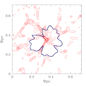
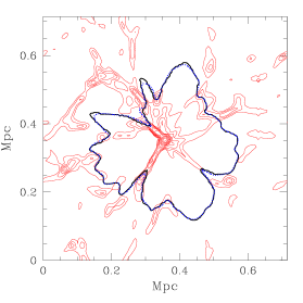
Figure 16: Full radiative transfer results from our method (thick dotted blue line) vs. explicit I-front tracking (thick solid black line) at times $t=0.5$ Myr (left) and $t=1$ Myr (right). Also shown are the density contours of the underlying density field (thin red lines).

We compare the results from the two methods as applied to the case of a single ionizing source in a cosmological density field (see § 6.2 for more details on the simulations). Since the explicit I-front tracking assumes sharp I-fronts and fixed temperature, for closest direct comparison with the results of our method for the same test we assumed an ionizing source with a soft black-body spectrum with effective temperature $T_{\rm eff}=20,000$ K. The gas temperature is fixed to $T=10^{4}$ K everywhere. In Fig. 16 we show the positions of the I-fronts obtained by the two methods at times $t=0.5$ Myr and 1 Myr. The dotted blue lines show the I-front calculated with full radiative transfer method, while the solid black lines show the I-front position according to the explicit I-front tracking. The thin red contours show the underlying density field. The H II regions assume a characteristic “butterfly” shape since the I-fronts, after they escape from the dense vicinity of the ionizing source, propagate faster in the voids and slower along the denser filaments. The results from the two methods show excellent agreement, thus verifying our ray-tracing procedure.

6 Some simple illustrative applications

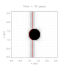
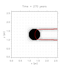
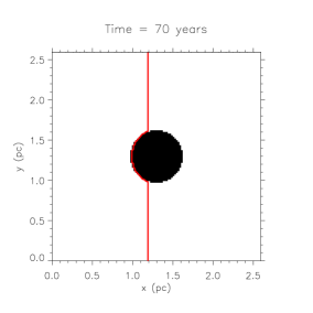
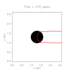
Figure 17: Plane parallel ionization front crossing a high density region. Top row: calculated on a 5-level adaptive mesh; Bottom row: calculated on a fixed mesh. The snapshots show the density in the central $xy$ plane (black=high density, white=low density), with the red contour showing the ionization front ($x=0.5$). In the AMR simulation the dark points indicate the computational mesh points.

6.1 Plane parallel ionization front on an adaptive mesh

Our radiative transfer and ray-tracing method are directly applicable to any type of rectangular mesh, not just a uniform one, but also nested and adaptively-refined (AMR) meshes. We have currently implemented it for a plane-parallel I-front on an AMR mesh, in addition to the fixed, uniform mesh case.

To illustrate the performance of our method on an adaptive mesh, we ran a simulation of a plane-parallel ionization front overrunning a dense spherical cloud. This problem was calculated both with a fixed mesh version, and with an adaptive mesh. The AMR method used is the one implemented in the Yguazu code (Raga et al. 2000b). It refines on a point by point basis, based on a given set of quantities, determined by the user (these could include e.g. pressure, density, ionized fractions of various species, etc.) and employs refinement steps of a factor of two. For this particular simulation we used a 3D box with sides of $8\times 10^{18}$ cm, filled with uniform gas of 5 cm^-3 and containing a ten times denser cloud of radius $10^{18}$ cm positioned in the center of the computational volume. We used five refinement levels, and the maximum resolution (at finest refinement level) is $128^{3}$. We refined on the gradients of the ionization fraction and density. For comparison we also ran the same problem on a fixed, uniform mesh of $128^{3}$ cells.

In Figure 17 we show the comparison between the AMR and the fixed mesh simulation results. Our AMR implementation correctly identifies both the I-front and the clump and refines around them. The I-front position and shape are identical at both times in the AMR and fixed-mesh results. This test demonstrates that our method interacts correctly with the adaptive mesh and properly tracks the I-front. For this particular problem the AMR simulation was completed approximately 10 times faster than the fixed mesh simulation, demonstrating the power of mesh adaptivity to speed up codes without loss of accuracy. Further tests and full description of the AMR implementation of C²-Ray will be presented in a subsequent paper which will discuss the direct coupling of our radiative transfer method with hydrodynamics (Iliev et al. 2005b).

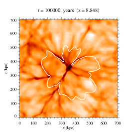
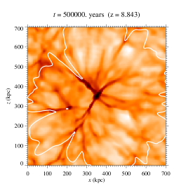
Figure 18: I-front propagation around a single ionizing source in a cosmological density field at times $t=0.1$ Myr (left) and $t=0.5$ Myr (right). Image is a cut through the source $y$-plane and shows the color-coded gas density field (the darker regions are denser). The current position of the I-front is indicated by the white line. See Movies 1–3 for an animated view of the growth of these ionization fronts in three planes.

6.2 Reionization of a cosmological density field

As a further illustration and testing of our code, we have applied our method the simulation of reionization of a fixed cosmological density field at redshift $z=8.85$. The gas distribution was obtained from a PM+TVD N-body and gasdynamical simulation (Shapiro et al. 2005a) performed using the cosmological dynamics code described in Ryu et al. (1993). The simulation box size is $0.5\,h^{-1}$ Mpc, the resolution is $128^{3}$ cells, $2\times 64^{3}$ particles.

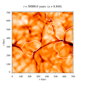
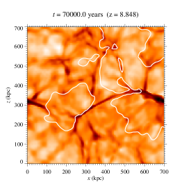
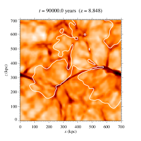
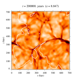
Figure 19: Ionization of a cosmological gas density distribution by multiple sources at time $t=0.05$ Myrs (top left) $t=0.07$ Myrs (top right), $t=0.09$ Myrs (bottom left), and $t=0.2$ Myrs (bottom right). Image shows the color-coded gas density field, cut through the middle of the box ($y$-plane). The current position of the I-fronts is indicated by the white lines. Movies 4–6 show the growth of these ionization in three planes through the center of the volume.

We ran two simulations, the first one with a single ionizing source in the computational volume, the other with multiple sources. For the single-source run the ionizing source is positioned at the highest-density point of the grid (which for visualization purposes is moved to the middle of the grid using the periodic boundary conditions), with luminosity $L=10^{9}L_{\odot}$ and black-body spectrum of effective temperature $T_{\rm eff}=50,000$ K, as appropriate for a massive Pop II star, corresponding to an ionizing photon production rate of $\dot{N}_{\gamma}=6.822\times 10^{52}\,\rm s^{-1}$. For the multiple-source run the ionizing sources are chosen to be the 6 most massive halos found in the box, with masses above $4\times 10^{7}M_{\odot}$, which mass at that redshift corresponds to a halo virial temperature $10^{4}$ K (Iliev & Shapiro 2001), below which temperature the gas cannot cool efficiently and form stars easily. The halos in the simulation box were found using a friends-of-friends halo finder with a linking length of 0.25. The ionizing photon production rate for each source is constant in time and is assigned assuming that each source lives $t_{s}=3$ Myr and has a constant mass-to-light ratio, emitting a total of $f_{\gamma}=250$ ionizing photons per atom during its lifetime, as is appropriate for massive stars (Iliev et al. 2005c):

$$\dot{N}_{\gamma}=f_{\gamma}\frac{M\Omega_{b}}{\Omega_{0}m_{p}t_{s}},$$ (38)

where $M$ is the total halo mass and $m_{p}$ is the baryon mass. The source cell is assigned to the densest cell inside the $3^{3}$ cells centered on the halo position. For simplicity all the sources are assumed to ignite at the same time.

In the single-source case, the the H II region is initially confined to the dense region around the source. Once most of the gas there is ionized, the I-front quickly escapes into the lower-density voids, while the denser filaments temporarily trap it and become ionized only slowly, creating a characteristic “butterfly” shape (Fig. 18). Later on the H II region becomes somewhat more spherical and eventually most of the computational box becomes ionized at $t\sim 1$ Myr.

Figure 20: Ionized gas fraction for (a)(left) single-source and (b)(right) multiple ionizing sources on a cosmological density field: mass-weighted, $x_{m}$, (solid) and volume-weighted, $x_{v}$ (dashed) (bottom panels) and their ratio (top panels).

When multiple ionizing sources are present in the computational volume (Fig. 19), the topology of the H II regions changes and becomes much more complex. Initially, individual H II regions form around each source, but due to the significant source clustering at high redshift these small isolated H II regions quickly merge into a few larger ones, with some remaining neutral pockets of denser gas along the filaments inside them which temporarily self-shield and trap the propagating I-front. The shape of the H II regions is quite non-spherical at all times, dictated by the interplay between the source clustering and the underlying density distribution. The computational domain becomes completely ionized within $\sim 1$ Myr.

This shows that reionization is not as simple as either “inside-out”– dense regions ionized first, low-density regions last – or “outside-in” – low-density regions, or voids, ionized first, dense regions last, claimed by Miralda-Escudé et al. (2000). The dense regions in the immediate vicinity of the sources were ionized first, but then the I-fronts quickly escaped into the voids, and thereafter the overdense and under-dense regions were being ionized simultaneously. This point is further illustrated in Figure 20, which shows the mass- and volume-weighted ionized fractions for both the single- and the multiple-source runs. Initially, in both cases the mass-weighted ionized fraction is significantly larger than the volume-weighted one. However, the ratio quickly, within 0.1-0.2 Myr, drops to $\sim 1$. The evolution is somewhat different thereafter. In the single-source case the ratio becomes somewhat less than one, as the voids become ionized faster than the dense regions. In the multiple-source case, on the other hand, the ratio stays very close to 1, indicating that while the voids (which take most of the volume) are ionized relatively quickly, the dense knots and filaments (which contain most of the gas mass) are also being ionized at the same time, which keeps the ratio of the mass- to volume-ionized fraction similar. With this simple example we thus confirm the results of e.g. Razoumov et al. (2002).

7 Conclusions

We presented a new method, called C²-Ray, for photoionization calculations and radiative transfer in optically-thick media. Our method is explicitly photon-conserving, which allows us to relax the often-required condition for the computational cells to be optically-thin, and thus be able to obtain accurate results even for very coarse spatial discretizations. Furthermore, we introduced time-averaged optical depths, which we obtain from a relaxation solution of the non-equilibrium chemistry equations, which allow us to use similarly coarse time-discretizations without any significant loss of accuracy. These developments result in a very fast, efficient and accurate calculation of the evolution of the ionization state of a gas distribution regardless of the spatial- and time-resolution.

We tested our method systematically, and in significant detail, in several astrophysically relevant situations in both 1D (in order to test its basic functionality) and in full 3D, at various resolutions in time and space. We compared the results against the corresponding exact analytical solutions, some of which we derived here for the first time. The results of these tests show that our method follows the analytical solutions to within a few percent, and conserves photons with the same accuracy or better, even when using extremely coarse grids and very long time steps. We have also shown that our radiative transfer method can be combined with adaptive mesh refinement (AMR), which leads to substantial increase in the calculation speed and much lower memory requirements. These tests demonstrate the importance of extensive testing of RT codes in a wide range of density fields - both for code validation and for possible adjustments of free parameters for better handling of special cases, e.g. steep density gradients. A project to thoroughly compare different codes used for cosmological radiative transfer methods is underway (Iliev et al. 2005, in preparation).

Our radiative transfer method imposes no limitations on the computational cell size and optical depth, and imposes no hard limits on the time step sizes. The only requirements we found are related to the desired accuracy of the solution obtained, for high accuracy the time step should be significantly shorter than the local recombination time. Longer time steps, comparable to the recombination time, lead to gradual loss of accuracy, but no incorrect or unstable solutions.

As a first simple application, we studied the reionization of a cosmological density field by both a single- and multiple-sources confirmed the findings of e.g. Razoumov et al. (2002) that neither inside-out, nor outside-in models describe the progress of cosmological I-fronts correctly. We showed that, instead, the mass- and volume-weighted ionized gas fractions are generally very similar, indicating that the dense and underdense regions are ionized at the same time.

The accurate I-front tracking over long time steps and coarse spatial resolutions makes our code ideal for direct dynamical coupling to multi-dimensional gasdynamics and N-body codes, where the evolution time-scales are generally much longer than the ionization and I-front crossing times. Allowing for larger, optically-thick cells further relaxes the time step limits imposed on the gasdynamic evolution through the Courant condition. In a follow-up paper we will address how we combine our C²-Ray method with 3D gas- and N-body dynamics, including more details on the coupling to AMR and calculating the effects of photo-ionization heating.

The C²-Ray’s high computational efficiency and correct I-front evolution over long time steps make it also a very attractive tool for studying reionization using high-resolution precomputed density fields. As a ray-tracing method, its performance scales linearly with the number of ionizing sources and the number of computational cells, but our tests show that on the available hardware we can perform such post-processing calculations on large computational meshes of $400^{3}$ to $800^{3}$ cells and for thousands of ionizing sources. In a future paper we will describe the results of these calculations and show how we use them to make detailed observational predictions e.g. for the large-scale 21-cm signal from the Epoch of Reionization.

GM is grateful to CITA and the LKBF for providing support for visits to CITA where significant part of this work was completed. The work of GM is partly supported by the Royal Netherlands Academy of Arts and Sciences. During the initial stages of this work ITI was supported in part by the Research and Training Network “The Physics of the Intergalactic Medium” established by the European Community under the contract HPRN-CT2000-00126. This work was partially supported by NASA grants NAG5-10825 and NNG04G177G and Texas Advanced Research Program grant 3658-0624-1999 to PRS. MAA is grateful for the support of the US Department of Energy Graduate Fellowship in Computational Sciences.

Appendix A Ray tracing

Here we describe how the column densities for a given cell are constructed using the short-characteristics method. For this we consider a point $d$ with position $(x,y,z)$ at mesh position $(i,j,k)$, see Fig. 21. The source point $s$ in physical coordinates is $(x_{\rm s},y_{\rm s},z_{\rm s})$ or in mesh coordinates $(i_{\rm s},j_{\rm s},k_{\rm s})$. The point where the ray enters the cell is called $c$. Assuming that the cells are cubical, the ray calculation is most easily done in mesh coordinates, which is what we will use.

For our method we need two column densities for each cell, the column density to the cell, called $N_{c}$ and the column density over the cell, denoted $\Delta N$. $N_{c}$ corresponds to the optical depth $\tau_{\nu}$, and $\Delta N$ corresponds to $\Delta\tau_{\nu}$ in Eq. (6).

$\Delta N$ is simply given by the $n_{\rm HI}{\rm d}s$, with ${\rm d}s$ the path length ${\rm d}s$ through the cell, which is twice the distance between $c$ and $d$ and can be shown to be

$${\rm d}s=\sqrt{1+{(i-i_{\rm s})^{2}+(j-j_{\rm s})^{2}\over(k-k_{\rm s})^{2}}}$$ (39)

in units of cell size. The appropriate value for $V_{\rm shell}$ in Eq. (6) is then given by $4\pi r_{sd}^{2}{\rm d}s$, where $r_{sd}$ is the distance between the source and the point $d$.

The column density to the cell $N_{c}$ is constructed from the column densities of the neighboring cells. In order to pick the correct neighbors, we need to establish where the ray enters the cell around $d$. This can be done using the differences $\Delta i=i-i_{\rm s}$, $\Delta j=j-j_{\rm s}$, $\Delta k=k-k_{\rm s}$ which show whether the ray from the source enters the cell through the $x$, $y$, or $z$ plane. E.g. if $|\Delta k|>|\Delta j|$ and $|\Delta k|>|\Delta i|$ the crossing is on the constant $z$-plane. Considering this case we calculate the point $c$ where the ray enters the cell, with mesh coordinates $(i_{c},j_{c},k_{c})$, where $k_{c}=k-{1\over 2}\sigma_{k}$ and $\sigma_{k}={|\Delta k|\over\Delta k}$.

The neighbors closer to the source are the four cells with mesh positions $e1$: $(i,j,k-\sigma_{k})$, $e2$: $(i,j-\sigma_{j},k-\sigma_{k})$, $e3$: $(i-\sigma_{i},j,k-\sigma_{k})$, and $e4$: $(i-\sigma_{i},j-\sigma_{j},k-\sigma_{k}$), with $\sigma_{i,j}={|\Delta i,j|\over\Delta i,j}$. From these we construct the column density at the crossing point $c$:

$$N_{c}=w_{1}N_{e1}+w_{2}N_{e2}+w_{3}N_{e3}+w_{4}N_{e4}\,,$$ (40)

with $w_{i}$ a set of normalized weights. These weights can be constructed in different ways. The most straightforward one is taking the $x$ and $y$ distances from point $c$ to the corner points:

$$\begin{array}[]{l}{\delta}_{i}=2|i_{c}-i+\sigma_{i}/2|\\ {\delta}_{j}=2|j_{c}-j+\sigma_{j}/2|\end{array}$$ (41)

and using

$$\begin{array}[]{l}w_{1}=(1-\delta_{i})(1-\delta_{j})\\ w_{2}=\delta_{i}(1-\delta_{j})\\ w_{3}=(1-\delta_{i})\delta_{j}\\ w_{4}=\delta_{i}\delta_{j}\end{array}$$ (42)

With this weighting $N_{c}=N_{e1}$ if the ray is parallel to the $z$-axis, and $N_{c}=N_{e4}$ if the ray travels diagonally over the mesh.

However, we found that this simple geometric weighting in case of a very clumpy medium gives too much spreading of shadows. As discussed previously in Raga et al. (1999), we suppress this by adding an extra optical-depth-dependent factor in the weights $w_{1}-w_{4}$.

$$\begin{array}[]{l}w_{1}={(1-\delta_{i})(1-\delta_{j})\over{\rm max}(\tau_{0},\tau_{e1})\sum_{n}w_{n}}\\ w_{2}={\delta_{i}(1-\delta_{j})\over{\rm max}(\tau_{0},\tau_{e2})\sum_{n}w_{n}}\\ w_{3}={(1-\delta_{i})\delta_{j}\over{\rm max}(\tau_{0},\tau_{e3})\sum_{n}w_{n}}\\ w_{4}={\delta_{i}\delta_{j}\over{\rm max}(\tau_{0},\tau_{e4})\sum_{n}w_{n}}\end{array}$$ (43)

The value of $\tau_{0}$ was determined empirically at 0.6. For this number we get the best photon-conservation for general clumpy media, when there are no strong density gradients present. In all tests and applications presented in this paper we use the weightings in Eq. (43), unless otherwise noted.

Figure 21: Short-characteristics ray tracing.

In the special case of density field with strong density gradients (e.g. $n\propto r^{-2}$, as in one of the tests we discuss in § 5) combined with low spatial resolution, the weightings in Eq. (43) with $\tau_{0}=0.6$ do not produce good photon conservation. This is easy to understand since steep density gradients combined with very coarse resolution lead to incorrect representation of the density field on the grid and of significant grid-induced anisotropies, which are only worsened by the weightings in Eq. (43). In such cases it is better to use the weightings in Eq. (43) with a small value for $\tau_{0}$ ($\tau_{0}=\epsilon>0$), i.e. essentially the weightings in this case are simply inversely proportional to the corresponding optical depths (or, equivalently, column densities), since ${\rm max}(\tau_{0},\tau_{e,i})=\tau_{e,i}$ for $i=1,4$. When the spatial resolution is sufficiently high (e.g. $128^{3}$ or $256^{3}$ mesh in the tests discussed in § 5) both types of weightings work well and produce almost identical results, with very high level of photon conservation, generally better than 1%, regardless of the time resolution employed.

For $|\Delta j|>|\Delta k|$ and $|\Delta j|>|\Delta i|$ we are dealing with a $y$-plane crossing and for $|\Delta i|>|\Delta k|$ and $|\Delta i|>|\Delta j|$ with an $x$-plane crossing. For these two cases the calculations are done in a similar way as above, but with the $y$ and $x$ coordinates taking the role of the $z$ coordinate, respectively.

Both the short characteristic method (which uses the column densities from the neighbors, as described above), and the time-averaged optical depth calculation, require the ray-tracing to be causal. To achieve this the mesh has to be traversed in a particular order, as described in Raga et al. (1999): we first trace away from the source along the $x$-axis ($y=y_{\rm s}$, $z=z_{\rm s}$), next we do strips of constant $y$ parallel to the $x$-axis. After the source plane ($z=z_{\rm s}$) has been traced, we move to $z$-planes away from the source, and trace each plane in the same way as the source plane. Since each cell has its own ray segment, the short characteristics method scales with the number of cells in the computational mesh.

A.0.1 Shadowing by a Dense Gas Cloud and I-front trapping

Some of the main effects due to radiative transfer in realistic simulations are slowing and possible trapping of the I-front in denser regions and the corresponding casting of shadows behind these dense regions. In this section we are testing our numerical scheme in such a situation. We use the initial conditions from Test 1 in Table 1, except that the computational box is 1 Mpc in size. We position a dense (gas number density $n=10^{3}\,\rm cm^{-3}$), uniform, rectangular slab with size $2\times 20^{23}$ by $5\times 10^{23}$ by $5\times 10^{23}$ cm at a distance 0.083 Mpc from the source (sizes are arbitrary and have no particular physical significance). The temperature is fixed at $t=10^{4}$ K everywhere. Results for a $128^{3}$ mesh are shown in Figure 22. As expected, the I-front is trapped inside the dense region within one cell. The shadows cast are clean and sharp, with only modest spurious diffusion in the shadow behind the clump. The I-front outside the shadow is not affected by its existence and keeps its original, perfectly circular shape.

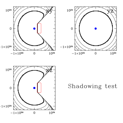
Figure 22: Shadows test. Same parameters as in Test 1 above, but introducing a dense ($n=10^{3}\rm cm^{-3}$) uniform slab (red) for resolution of $128^{3}$ cells. Source is in the middle of the computational box (blue circle). Contours are of the 50% ionized fraction in a time-sequence from $t=20$ Myr to 100 Myr, with intervals of 20 Myrs. The thicker line is for $t=20$ Myrs and its thickness indicates the width of the ionization front. The three panels for each case are cuts through the center along $x$-$y$, $y$-$z$ and $x$-$z$ plane, as labeled.

References

- Abel et al. (1999) Abel, T., Norman, M. L., & Madau, P. 1999, ApJ, 523, 66
- Bolton et al. (2004) Bolton, J., Meiksin, A., & White, M. 2004, MNRAS, 348, L43
- Cen (2002) Cen, R. 2002, ApJS, 141, 211
- Chevalier & Dwarkadas (1995) Chevalier, R. A. & Dwarkadas, V. V. 1995, ApJ, 452, L45
- Ciardi et al. (2000) Ciardi, B., Ferrara, A., Governato, F., & Jenkins, A. 2000, MNRAS, 314, 611
- Ciardi et al. (2003) Ciardi, B., Stoehr, F., & White, S. D. M. 2003, MNRAS, 343, 1101
- Dopita & Sutherland (2003) Dopita, M. A. & Sutherland, R. S. 2003, Astrophysics of the diffuse universe (Astrophysics of the diffuse universe, Berlin, New York: Springer, 2003. Astronomy and astrophysics library, ISBN 3540433627)
- Franco et al. (1990) Franco, J., Tenorio-Tagle, G., & Bodenheimer, P. 1990, ApJ, 349, 126
- Frank & Mellema (1994) Frank, A. & Mellema, G. 1994, A&A, 289, 937
- Gnedin & Abel (2001) Gnedin, N. Y. & Abel, T. 2001, New Astronomy, 6, 437
- Hayes & Norman (2003) Hayes, J. C. & Norman, M. L. 2003, ApJS, 147, 197
- Henney & Arthur (1998) Henney, W. J. & Arthur, S. J. 1998, AJ, 116, 322
- Iliev et al. (2005a) Iliev, I. T., Hirashita, H., & Ferrara, A. 2005a, MNRAS, submitted (astro-ph/0509261)
- Iliev et al. (2005b) Iliev, I. T., Mellema, G., & Shapiro, P. R. 2005b, in preparation
- Iliev et al. (2005c) Iliev, I. T., Scannapieco, E., & Shapiro, P. R. 2005c, ApJ, 624, 491
- Iliev & Shapiro (2001) Iliev, I. T. & Shapiro, P. R. 2001, MNRAS, 325, 468
- Iliev et al. (2005d) Iliev, I. T., Shapiro, P. R., & Raga, A. C. 2005d, MNRAS, 361, 405
- Lim & Mellema (2003) Lim, A. J. & Mellema, G. 2003, A&A, 405, 189
- Maselli et al. (2003) Maselli, A., Ferrara, A., & Ciardi, B. 2003, MNRAS, 345, 379
- Mellema (1994) Mellema, G. 1994, A&A, 290, 915
- Mellema et al. (1998) Mellema, G., Raga, A. C., Canto, J., Lundqvist, P., Balick, B., Steffen, W., & Noriega-Crespo, A. 1998, A&A, 331, 335
- Miralda-Escudé et al. (2000) Miralda-Escudé, J., Haehnelt, M., & Rees, M. J. 2000, ApJ, 530, 1
- Nakamoto et al. (2001) Nakamoto, T., Umemura, M., & Susa, H. 2001, MNRAS, 321, 593
- Navarro et al. (1997) Navarro, J. F., Frenk, C. S., & White, S. D. M. 1997, ApJ, 490, 493
- Osterbrock (1989) Osterbrock, D. E. 1989, Astrophysics of gaseous nebulae and active galactic nuclei (Research supported by the University of California, John Simon Guggenheim Memorial Foundation, University of Minnesota, et al. Mill Valley, CA, University Science Books, 1989, 422 p.)
- Raga et al. (2000a) Raga, A., López-Martín, L., Binette, L., López, J. A., Cantó, J., Arthur, S. J., Mellema, G., Steffen, W., & Ferruit, P. 2000a, MNRAS, 314, 681
- Raga et al. (1999) Raga, A. C., Mellema, G., Arthur, S. J., Binette, L., Ferruit, P., & Steffen, W. 1999, Revista Mexicana de Astronomia y Astrofisica, 35, 123
- Raga et al. (1997) Raga, A. C., Mellema, G., & Lundqvist, P. 1997, ApJS, 109, 517
- Raga et al. (2000b) Raga, A. C., Navarro-González, R., & Villagrán-Muniz, M. 2000b, Revista Mexicana de Astronomia y Astrofisica, 36, 67
- Razoumov et al. (2002) Razoumov, A. O., Norman, M. L., Abel, T., & Scott, D. 2002, ApJ, 572, 695
- Razoumov & Scott (1999) Razoumov, A. O. & Scott, D. 1999, MNRAS, 309, 287
- Ryu et al. (1993) Ryu, D., Ostriker, J. P., Kang, H., & Cen, R. 1993, ApJ, 414, 1