Going Nonlinear with Dark Energy Cosmologies

Abstract

We propose an efficient method for generating high accuracy ($\sim 1\%$) nonlinear power spectra for grids of dark energy cosmologies. Our prescription for matching matter growth automatically matches the main features of the cosmic microwave background anisotropy power spectrum, thus naturally including “CMB priors”.

I Introduction

The formation of large scale structure in the universe is a central element of astrophysics. Apart from the structure itself, it also offers a incisive tool for probing cosmology and particle physics. Since structure formation is a competition between expansion and gravity, the growth as a function of redshift is intimately tied to the expansion of the universe. Studies of matter density fluctuations can thus shed light on the physics responsible for the accelerating expansion, i.e. dark energy. The growth of large scale structure also provides one of the few tests of general relativity on cosmological scales.

One of the most informative descriptions of large scale structure, and the most widely used, is the power spectrum of density fluctuations. The power spectrum can be probed through observations including galaxy and cluster redshift surveys, weak gravitational lensing, baryon acoustic oscillations, the Lyman alpha forest, etc. To translate the measured power spectrum to a cosmological model, one needs accurate predictions for the power spectrum in a variety of dark energy cosmologies. This typically comes from large simulations, and fitting forms derived from such simulations. However the multitude of possible dark energy cosmologies is vast, and the necessary simulations are computationally expensive. The first dynamical dark energy simulations appeared only in 2003 linjen ; klypin and even constant dark energy equation of state model simulations exist for only a handful of models. Fitting forms, such as in pkfit , are tuned to the cosmological constant model and even then agree with simulations to only $\sim 10\%$.

To use the next generation of large scale structure observations we need a better, more efficient method of predicting the effects of cosmology on the power spectrum. Section II presents a new prescription for this, reducing the dimensionality of the grid of cosmologies that need simulation. In §III we present the results of simulations, obtaining $\sim 1\%$ accuracy in the matter power spectra. The method is extended in §IV with a discussion of time varying equations of state and cosmic microwave background anisotropies.

II Going Nonlinear

In general relativity the power spectrum of linear matter density perturbations can be readily calculated (see SSWZ for a recent convergence study). On large scales and at late times the power spectrum grows with fixed shape and the growth function can be evaluated, even for dynamical dark energy cosmologies, from a simple differential equation linjen or highly accurate fitting formulas groexp . This remains true even for some extended theories of gravity groexp . Since nonlinear structures develop from linear perturbations, the linear growth function is a natural place to start.

Given two cosmological models, we can match their growth factors at the present by normalizing to the same mass fluctuation amplitude, $\sigma_{8}$. For definiteness, consider matching some dark energy model, characterized by its equation of state or pressure to energy density ratio, $w=p/\rho$, to a cosmological constant ($w=-1$) cosmology with dimensionless matter density $\Omega_{m}=0.3$ (we assume spatial flatness for all models). Next we match the normalized growth factors $\tilde{g}(a)$ at a second scale factor. This scale factor, $a_{\star}$, is chosen to minimize the deviation between the models’ linear growth factors over some redshift range. For the range $z=0-3$, we find $a_{\star}=0.35$, or $z_{\star}=1.86$, is a good choice. One could choose a different range and obtain a different $a_{\star}$.

Matching the $\tilde{g}(a_{\star})$ determines a value of $\Omega_{m}$ for the dark energy model. Finally, we fix the Hubble constant by keeping $\Omega_{m}h^{2}$ the same for the two models. Table 1 shows the results for various dark energy cosmologies.

The degeneracy relation upon changing $w$, or $\Omega_{m}$, between two constant equation of state models is

$$\Delta\Omega_{m}\approx 0.42(1-a_{\star})\Delta w.$$ (1)

For example, if the models differ by 0.02 in $\Omega_{m}$, they must also differ by 0.096 in $w$ to match growths at, say, $z=1$ (generalizing $a_{\star}$). This is only a rule of thumb (e.g. a coefficient 0.39 works better for $w<-1$ models and 0.44 for $w>-1$ models), good near the fiducial $\Omega_{m}=0.3$, $w=-1$. However it is easy to compute the matching numerically, and we use the exact calculation throughout.

$\Omega_{m}$	$h$	$w_{0}$	$w_{a}$	$10^{5}\delta_{H}$
0.3	0.7	-1	0	5.0
0.26	0.7519	-1.156	0	5.769
0.28	0.7246	-1.076	0	5.357
0.32	0.6778	-0.929	0	4.688
0.34	0.6575	-0.861	0	4.412
0.3846	0.6182	-0.8	0.3	3.900
0.3356	0.6618	-0.8	-0.3	4.470
0.3214	0.6763	-1.0	0.3	4.667
0.2808	0.7235	-1.0	-0.3	5.342

Table 1: Cosmological parameters generated from our prescription for matching the nonlinear power spectra of dark energy cosmologies. The last column is defined as the present day value of the dimensionless power spectrum at $k=H$, i.e. $\Delta^{2}(k)=\delta_{H}^{2}(k/H)^{3+n}T^{2}(k)$, where we adopt scale invariance $n=1$, and $T(k)$ is the transfer function EisHu , fixed for $k$ measured in 1/Mpc.

III Results from Simulations

By working at constant $\Omega_{m}h^{2}$ and $\Omega_{b}h^{2}$ we fix the shape of the matter power spectrum in physical units, e.g. $k$ in Mpc^-1. Our procedure arranges a close match of the growth of the power spectrum in the linear regime. Thus it is natural to expect that the nonlinear power spectra will be closely matched. To test this we make use of N-body simulations.

For the first 5 models of Table 1 we ran N-body simulations using a parallel particle-mesh (PM) code PM . In each case we evolved $256^{3}$ equal mass particles using a $512^{3}$ force mesh from $z=60$ to the present, dumping the phase space data at $z=1.86$, 1, and 0. The simulation volume for the results presented here was a periodic, cubical box of side 366 Mpc, though we also ran a few larger boxes to check convergence on the largest scales. For each output time, the power spectrum was computed by assigning the particles to the nearest grid point of a regular, $512^{3}$ Cartesian mesh and Fourier transforming the resultant density field. The resulting $\Delta^{2}(k)$, corrected for the assignment to the grid using the appropriate window function and for Poisson shot noise, were placed in logarithmically spaced bins of $k$. The average $\Delta^{2}(k)$ is plotted at the position of the average $k$ in each bin.

While the PM code has limited force resolution, it allows high mass resolution at modest computational cost. This is important in the translinear scales ($\Delta^{2}\sim 1$) of interest here. The finite force and mass resolution of the PM code limits the dynamic range in $k$ to $\sim 50$, and the short-fall in power can be easily seen in the highest $k$ point plotted in the top left panel of Fig. 1. Much of the effect of the force resolution is reduced in taking the ratio (see also McDonald ) of power spectra, as in the lower panels of Fig. 1, although the details of the shot-noise correction are starting to become important on these scales.

From Fig. 1 we see that across most of the range of scales probed by, e.g., weak lensing and for which we believe purely gravitational N-body simulations will provide accurate calculations of the power spectrum, the models are indeed nearly degenerate. The maximum deviation in $\Delta^{2}(k)$ is 1.5%, for the $\Omega_{m}=0.26$, $w=-1.156$ model at $z=0.5$. This is also the maximum deviation in the (square of the) linear theory growth rates. Where the growth rates are closely matched, the nonlinear power spectra are too.

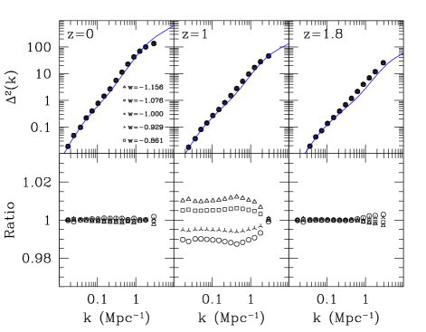
Figure 1: The nonlinear mass power spectrum is shown at three redshifts. The top panels plot $\Delta^{2}(k)=k^{3}P_{k}/(2\pi^{2})$ from the simulations for five different dark energy models matched according to our prescription. The solid line indicates the Smith et al. pkfit fitting formula. The bottom panels show the ratio of $\Delta^{2}(k)$ for the four dark energy models relative to the $\Lambda$CDM case.

IV Growth and the CMB

A significant new result is that the distance to last scattering $d_{\rm lss}$ is automatically preserved through our matching prescription. That is, by matching the growth today and at $a_{\star}=0.35$, we ensure that $d_{\rm lss}$ changes very little; the growth factor determines the distance. The fractional distance deviation of the dark energy models from the $\Lambda$CDM case is less than $0.04\%$ (e.g. 0.001% for the $\Omega_{m}=0.28$, $w=-1.076$ case).

This is important because the CMB is one of our strongest probes of large scale structure and cosmology. The main impact of the dark energy and the matter density on the CMB power spectrum is through the geometric degeneracy involving the distance to the last scattering surface, and the physical matter density $\Omega_{m}h^{2}$. Our prescription takes care of both, meaning that we select models that automatically include a strong CMB prior (see also LensGrid ): our matched models, with $\Omega_{m}h^{2}$ and $d_{\rm lss}$ fixed, will agree on the CMB temperature power spectrum to high accuracy, except at low multipoles where the integrated Sachs-Wolfe effect enters (though cosmic variance makes differences hard to detect) and at high multipoles through the effect of gravitational lensing.

We can further extend this to models with time varying dark energy equation of state. For values of $w_{0}$ and $w_{a}$, where $w(a)=w_{0}+w_{a}(1-a)$, we match the growth at the present and at $a_{\star}$ (we have checked that $a_{\star}=0.35$ works for these cases as well). This provides the necessary value of $\Omega_{m}$, and hence $h$ (see Table 1). For matching models with $(w_{0},w_{a})$ of $(-1,0.3)$, $(-1,-0.3)$, and $(-0.8,-0.3)$, the maximum deviation from the fiducial $\Lambda$CDM model in the linear growth factor is less than 0.6%, at $z=0.6$. So we expect, based on §III, that the nonlinear power spectra will match to within 1.2%. A matching model with $(-0.8,0.3)$, where the average equation of state lies further from the fiducial $w=-1$ and the required $\Omega_{m}$ is 30% different from the fiducial model, fits somewhat less well: the expected deviation in the nonlinear power spectrum is 3.4%.

The time varying equation of state models still preserve the CMB matching as well. They match on $d_{\rm lss}$ to better than 0.1%, except for $(-0.8,0.3)$ which agrees to 0.4%.

V Conclusion

We present a simple prescription for generating the nonlinear mass power spectrum of dark energy cosmologies, accurate to $\sim 1-2\%$. It requires only straightforward calculation of the linear growth factor at two redshifts. This will allow efficient generation of a suite of dark energy cosmologies using only a reduced dimension grid of $\Lambda$CDM simulations.

Moreover, we have identified a strong degeneracy between the growth factor and the CMB distance to last scattering, such that our matching procedure can automatically satisfy CMB constraints.

- (1) E.V. Linder & A. Jenkins, MNRAS 346, 573 (2003) [astro-ph/0305286]
- (2) A. Klypin, A.V. Macciò, R. Mainini, S.A. Bonometto, Ap. J. 599, 31 (2003) [astro-ph/0303304]
- (3) R.E. Smith et al., MNRAS 341, 1311 (2003) [astro-ph/0207664]
- (4) U. Seljak, N. Sugiyama, M. White, M. Zaldarriaga, Phys. Rev. D 68, 083507 (2003) [astro-ph/0306052]
- (5) E.V. Linder, Phys. Rev. D 72, xx (2005) [astro-ph/0507263]
- (6) D. Eisenstein, W. Hu, Ap. J. 511, 5 (1999)
- (7) R. Juszkiewicz, MNRAS 197, 931 (1981); E.T. Vishniac, MNRAS 203, 345 (1983)
- (8) F. Bernardeau, S. Colombi, E. Gaztañaga, R. Scoccimarro, Phys. Rep. 367 1 (2002) [astro-ph/0112551]
- (9) A. Meiksin, M. White, MNRAS 324, 141 (2001); A. Meiksin, M. White, MNRAS 342, 1204 (2003); A. Meiksin, M. White, MNRAS 350, 1107 (2004)
- (10) P. McDonald, H. Trac, C. Contaldi, preprint [astro-ph/0505565]
- (11) M. White, C. Vale, Astroparticle Physics 22, 19 (2004) [astro-ph/0312133]