N-body Simulations of the Magellanic Stream

Abstract

A suite of high-resolution N-body simulations of the Magellanic Clouds – Milky Way system are presented and compared directly with newly available data from the H i Parkes All-Sky Survey (HIPASS). We show that the interaction between Small and Large Magellanic Clouds results in both a spatial and kinematical bifurcation of both the Stream and the Leading Arm. The spatial bifurcation of the Stream is readily apparent in the HIPASS data, and the kinematical bifurcation is also tentatively identified. This bifurcation provides strong support for the tidal disruption origin for the Magellanic Stream. A fiducial model for the Magellanic Clouds is presented upon completion of an extensive parameter survey of the potential orbital configurations of the Magellanic Clouds and the viable initial boundary conditions for the disc of the Small Magellanic Cloud. The impact of the choice of these critical parameters upon the final configurations of the Stream and Leading Arm is detailed.

1 Introduction

The progressive collapse and merging associated with hierarchical clustering within a cold dark matter cosmology, while dominated by activity at early epochs (redshifts $z\sim 2$ – 5; e.g. Murali et al., 2002), continues to the present-day and is readily observable even in the local Universe. In our own Milky Way (MW), ongoing satellite disruption and accretion events include the Sagittarius dwarf (Ibata et al., 1994), the Canis Major dwarf (Martin et al., 2005, and references therein), and perhaps the most spectacular of all, the Large (LMC) and Small (SMC) Magellanic Clouds (MCs). The disruption and accretion of the MCs is perhaps best appreciated through the nearly circum-Galactic polar ring of gas – the Magellanic Stream – emanating from the Clouds (Mathewson et al., 1974; Putman et al., 1998).

Two primary, competing, scenarios have been postulated to explain the origin of the Magellanic Stream (MS): (i) ram pressure stripping of LMC and SMC gas due to the motion of the Clouds through the tenuous coronal gas in the Galactic halo (Moore & Davis, 1994; Mastropietro et al., 2005). This “drag” scenario faces difficulty in explaining the Leading Arm Feature (LAF) observed by Putman et al. (1998). (ii) tidal disruption of the SMC (Murai & Fujimoto, 1980). Because of its ability to simultaneously produce both trailing and leading streams of gas, the “tidal” model has gathered considerable support in the literature (Gardiner & Noguchi, 1996; Gardiner, 1999; Yoshizawa & Noguchi, 2003, hereafter, GN96, G99 and YN03 respectively).

Constraints upon theoretical models of the Magellanic Stream have improved dramatically with the release of the H i Parkes All-Sky Survey (HIPASS; Barnes et al., 2001) dataset. The extent and fine-scale structure of the MS can now be appreciated to a level not previously possible, in particular the unequivocal evidence for the existence of the Leading Arm Feature (Putman et al., 1998). Motivated by HIPASS, we have initiated a program of high-resolution N-body modelling of the Magellanic Stream aimed at de-constructing the temporal evolution of the Magellanic Clouds – Milky Way interaction. Here, we use $\sim 30$ times higher resolution than previous models such as GN96, G99 and YN03, giving us a H i mass resolution of $\sim 5600{\rm\,M}_{\sun}$ and a H i flux resolution of $7{\rm\,Jy\,{\rm\,km\,s}^{-1}{}}$. In addition, we construct a detailed H i map, to compare with the HIPASS data directly and quantitatively. The combination of a higher resolution simulation and the simulated H i map enables us to argue about more detailed features in the MS and the LAF. As a result, this paper shows more convincingly that the observed LAF and MS can be produced by the leading and trailing streams of the SMC, induced by tidal interactions with the MW and LMC. Our fiducial model is found after an extensive parameter survey of the potential orbital configurations of the MCs and the different initial condition of the SMC. Based on the parameter survey, we also demonstrate how the final features of the MS and the LAF are sensitive to the initial configuration of the SMC. Our new high-resolution simulations also reveal that the tidal interactions create spatial and kinematical bifurcation in the MS and LAF. We present this prediction based on our simulations, however we also demonstrate that the existing HIPASS data show such bifurcations.

The work described here (Paper I) is the first in a series of papers aimed at providing a definitive model for the MS and the LAF. Here, we concentrate solely upon the effects of gravity, describing the SMC disc with collisionless particles, and ignore the baryon physics (including hydrodynamics, star formation, energy feedback, and chemical enrichment). In Paper II, the effects of baryonic physics will be detailed.

The layout of this paper is as follows: in Section 2 we provide a description of the suite of simulations generated to date. In Section 3, we show the results from our best model, and compare them with the observational data. In Section 4, we demonstrate how the final features of the MS and LAF depend upon the orbits of the MCs and the initial properties of the SMC disc. Finally, in Section 5, the discussion and future directions for our work are presented.

2 Numerical Simulation

The framework upon which our simulations are based parallels that described by GN96 and YN03. The MW and LMC are taken to be fixed potentials, while the SMC is treated as an ensemble of self-gravitating particles, in recognition of the fact that the MS is thought to originate from the tidal disruption of the SMC disc (e.g. Gardiner et al., 1994, hereafter GSF94; GN96; Maddison et al., 2002; YN03; but see also Mastropietro et al., 2005). The orbits of the MW and LMC with respect to the SMC are pre-calculated, the procedure for which is outlined in Section 2.1 and GSF94. The initial boundary conditions for the “live” SMC model is described in Section 2.2, and its evolution explored in Section 2.3.

2.1 The orbits of the LMC and SMC

We assume a spherically symmetric potential for the MW halo. The MCs sample a volume of the halo where the gravitational potential is insensitive to both the expected central cusp and the outer regions where the density profile may be steeper than an isothermal profile. We hence assume a constant rotational velocity of $V_{\rm c}=220{\rm\,km\,s}^{-1}$ within the MW halo. Thus, the potential is described by

$$\phi_{\rm G}(r)=-V_{\rm c}^{2}\ln r$$ (1)

with a mass enclosed within $r{\rm\,kpc}$ of

$$M_{\rm G}(<r)=5.6\times 10^{11}\left(\frac{V_{\rm c}}{220{\rm\,km\,s}^{-1}}\right)^{2}\left(\frac{r}{50{\rm\,kpc}}\right){\rm\,M}_{\sun}.$$ (2)

We assume that there is little disc contribution to the potential at the typical Galactocentric distances of the LMC and SMC ($\sim 50{\rm\,kpc}$). The halos of both the MW and LMC are assumed to be invariant for the duration of the simulation ($2.5{\rm\,Gyr}$ – i.e., a lookback time corresponding to redshift $z\sim 0.2$). Plummer potentials are adopted for both the LMC and SMC – i.e.,

$$\phi_{\rm L,S}({\bf r})=GM_{\rm L,S}/\left[\left({\bf r}-{\bf r}_{\rm L,S}\right)^{2}+K_{\rm L,S}^{2}\right]^{1/2},$$ (3)

where ${\bf r}_{\rm L,S}$ are the positions of the Clouds relative to the MW centre, and $K_{\rm L,S}$ are the core radii, set to $3$ and $2{\rm\,kpc}$ for the LMC and SMC, respectively. In the fiducial model, we assume a constant mass of $M_{\rm L}=2\times 10^{10}{\rm\,M}_{\sun}$ for the LMC, and $M_{\rm S}=3\times 10^{9}{\rm\,M}_{\sun}$ for the SMC.

Adopting these parameters, we next backwards integrate the orbits of the SMC and LMC, using as boundary conditions the current tangential and radial velocities and positions of the Clouds listed in Table 1 (see also Murai & Fujimoto, 1980, GSF94, GN96, Lin et al., 1995 and Bekki et al., 2004). The values we adopted for our work were chosen to match those of GN96, and are consistent with the extant literature.

Table 1: Present-day orbital parameters for the SMC and LMC from the literature and values we have adopted in this work.

Parameter	LMC		SMC
	Literature	This	Literature	This
		work		work
$v_{\rm r,GSR}$	$84\pm 7$	$80.1$	$\sim 7$	$7.1$
$v_{\rm t,GSR}$	$281\pm 41$ ftn:vah+02	$287$	$200\pm 100$	$255$
$l$	$280.46\degr$	$280.46\degr$	$302.79\degr$ ftn:t88	$302.79\degr$
$b$	$-32.89\degr$ ftn:t88	$-32.89\degr$	$-44.30\degr$ ftn:t88	$-44.30\degr$
$d$	$49.43$	$49.43$	$57.02$ftn:fw87	$57.02$

The equations of motion of the Clouds about the stationary MW are

$$\ddot{\bf r}_{\rm L}=\frac{\partial}{\partial{\bf r}_{\rm L}}\left[\phi_{\rm S}\left(\left|{\bf r}_{\rm L}-{\bf r}_{\rm S}\right|\right)+\phi_{\rm G}\left(\left|{\bf r}_{\rm L}\right|\right)\right]+{\bf F}_{\rm L}/M_{\rm L}$$ (4)

and

$$\ddot{\bf r}_{\rm S}=\frac{\partial}{\partial{\bf r}_{\rm S}}\left[\phi_{\rm L}\left(\left|{\bf r}_{\rm S}-{\bf r}_{\rm L}\right|\right)+\phi_{\rm G}\left(\left|{\bf r}_{\rm S}\right|\right)\right]+{\bf F}_{\rm S}/M_{\rm S},$$ (5)

where the potentials $\phi_{\rm L}$, $\phi_{\rm S}$ and $\phi_{\rm G}$ refer to the Large and Small Magellanic Clouds, and the Galaxy, respectively (Murai & Fujimoto, 1980). Since we do not model the MW as live particles, dynamical friction is modelled as per GSF94. ${\bf F}_{\rm L}$ and ${\bf F}_{\rm S}$ are the dampening force between the Galaxy and each of the Clouds:

$${\bf F}_{\rm L,S}=\frac{-GM_{\rm L,S}}{\left|{\bf r}_{\rm L,S}\right|^{2}}\ln\left(\Lambda\right)\frac{\dot{\bf r}_{\rm L,S}}{\left|\dot{\bf r}_{\rm L,S}\right|}$$ (6)

$$\mbox{}\times\left\{\frac{2\left[\int_{0}^{x}{\exp(-y^{2})dy-\exp(-x^{2})x}\right]}{\pi^{1/2}x^{2}}\right\}_{x=\left[\left|\dot{\bf r}_{\rm L,S}\right|^{2}/V_{\rm c}\right]^{1/2}},$$

where $\ln(\Lambda)$ is the Coulomb logarithm.

Although equation (6) is a simple analytical formulation for dynamical friction that fails to model accurately the orbit of the Clouds for more than $5{\rm\,Gyr}$, according to recent studies (Hashimoto et al., 2003; Just & Peñarrubia, 2005), it gives a good approximation to the predictions of full N-body simulations over the $\sim 2.5{\rm\,Gyr}$ period we focus on in this paper. We note also, the strong effect the Coulomb logarithm has on the orbits. Hashimoto et al. (2003) suggest that the $\ln(\Lambda)$ value of 3 advocated by Binney & Tremaine (1987) for the LMC is too large, causing the system to evolve too fast. Thus, for this paper, we set $\ln(\Lambda)=1$ to enable direct comparison with the previous works.

Our fiducial model is initiated at a lookback time of $2.5{\rm\,Gyrs}$ when the Clouds are at apo-Galacticon (with the tidal forces between all three bodies being minimised). The subsequent orbit appears in Fig. 1, and the distance between the Clouds and Galaxy is shown in Fig. 2.

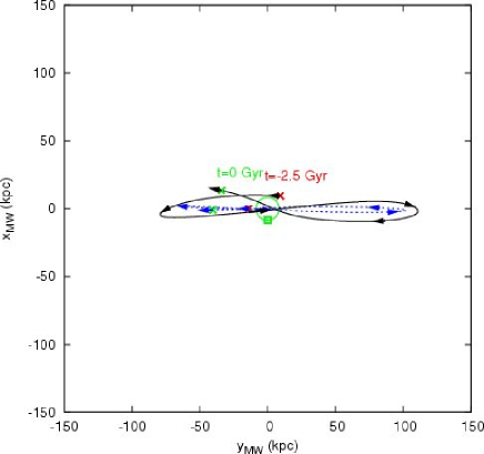
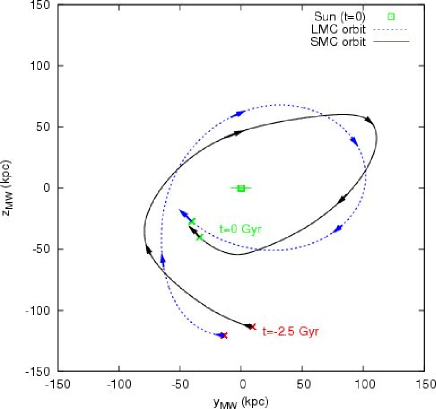
Figure 1: The three dimensional orbit of the SMC (black line) and the LMC (blue dashed line) around the Galaxy. The rotation axis of the MW is assumed to be the $z$-axis, and the disc plane is centred on $z=0$. The orbits, which are derived by backwards integrating to $T=-2.5{\rm\,Gyr}$, are plotted with arrows indicating each $0.5{\rm\,Gyr}$ between $T=0$ and $-2.5{\rm\,Gyr}$. The green crosses denote the current position of the SMC and LMC. The Solar radius at $8.5{\rm\,kpc}$ is also shown, and the current position of the Sun at $T=0$ is marked by the open square.

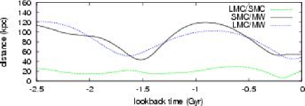
Figure 2: Distance (upper) and approximate tidal forces (lower; on a logarithmic scale in arbitrary units) between the three interacting bodies in our fiducial model.

Table 2: Fiducial SMC model parameters (see Kuijken & Dubinski, 1995 for details of parameters).

	Disc							Halo
	$M_{\rm d}$	$R_{\rm d}$	$R_{\rm t}$	$z_{\rm d}$	$\delta R_{\rm out}$	$\sigma_{\rm R,0}$		$\Psi_{0}$	$\sigma_{0}$	$q$	$C$	$R_{\rm a}$
	(${\rm M}_{\sun}$)	(${\rm kpc}$)	(${\rm kpc}$)	(${\rm kpc}$)	(${\rm kpc}$)	(${\rm km\,s}^{-1}$)		(${\rm km}^{2}{\rm s}^{-2}$)				(${\rm kpc}$)
	$2.47\times 10^{9}$	$3.5$	$7.0$	$0.35$	$1.1$	$35$		$-5.72\times 10^{3}$	$29$	$1.0$	$0.1$	$0.96$

2.2 SMC model

The initial dynamical configuration for the SMC was constructed using GalactICs (Kuijken & Dubinski, 1995). We employed a bulgeless equilibrium model with a truncated exponential disc, and a dark matter King-profile halo. The relevant GalactICs parameters for the fiducial SMC model appear in Table 2 (a detailed explanation of the individual parameters is provided by Kuijken & Dubinski, 1995). The disc possesses an exponential profile with scale radius $R_{\rm d}=3.5{\rm\,kpc}$, smoothly truncated beyond $R_{\rm t}=7{\rm\,kpc}$ (with 95 per cent of both the disc and halo masses being within $r_{\rm d,95}\sim r_{\rm h,95}\sim 7{\rm\,kpc}$), to give a disc with total radial extent (where the face-on surface density of the disc reaches $1{\rm\,M}_{\sun}{\rm\,pc}^{-2}$) of $7.5{\rm\,kpc}$ (compared to the halo with radial extent $\sim 14{\rm\,kpc}$). The rotation curve peaks at $\sim 2{\rm\,kpc}$ with a velocity of $\sim 45{\rm\,km\,s}^{-1}$, and turns over to become approximately constant, giving a total SMC mass of $3\times 10^{9}{\rm\,M}_{\sun}$, with the disc mass being $1.5\times 10^{9}{\rm\,M}_{\sun}$. The central velocity dispersion of the disc was chosen to be near the current H i velocity dispersion of the observed SMC (Fig. 8), and the dark matter halo velocity dispersion is similar to the value of $\sim 25{\rm\,km\,s}^{-1}$ obtained from observations of the stellar halo carbon stars and planetary nebulae (Dopita et al., 1985; Hardy et al., 1989; Hatzidimitriou et al., 1997). The Toomre $Q$-parameter at the disc half-mass radius is $Q=1.4$.

Our fiducial SMC model assumes a somewhat different scale length and total extent for the SMC disc when compared with earlier studies (GSF94; GN96; YN03). We should stress that one cannot simply take as initial conditions, observed parameters of the SMC at the present day, since the SMC has (obviously) been significantly disturbed by interactions with the MW and LMC; we instead use initial parameters consistent with other relatively isolated dwarf disc galaxies (and integrate forward to ensure the final characteristics is consistent with that observed today). Dwarfs with H i mass $1.3$ – $2.0\times 10^{9}{\rm\,M}_{\sun}$ (comparable to the SMC) have H i disc scale lengths ranging from $1.6$ to $4.4{\rm\,kpc}$, and smaller optical (i.e. stellar) scale lengths of $0.9$ to $2.7{\rm\,kpc}$ (Swaters et al., 2002). These same galaxies have H i discs whose face-on corrected H i density drops to $1{\rm\,M}_{\sun}{\rm\,pc}^{-2}$ at a radius between $10$ to $12{\rm\,kpc}$.

The reasons for the larger truncation radius compared to previous work are twofold. First, we suggest the tidal radius of the SMC disc is larger than the $5{\rm\,kpc}$ proposed by GN96. Several Gyrs ago, the MW was likely to have been slightly less massive (secular halo growth), the SMC slightly more massive (less tidal disruption), and the perigalactic distance of the SMC was larger. In the estimated orbit of the SMC, at a lookback time of $2.5{\rm\,Gyr}$ (Fig. 2), the perigalactic distance $r_{\rm p}$ was $60{\rm\,kpc}$, and the apogalactic distance $r_{\rm a}$ was $120{\rm\,kpc}$. However, the MW mass enclosed within the larger SMC orbit has then increased. The tidal radius of the SMC is (Faber & Lin, 1983)

$$r_{\rm t}=r_{\rm p}\left[\frac{M_{\rm S}}{(3+e)M_{\rm G}(r_{\rm p})}\right]^{1/3},$$ (7)

where the eccentricity $e=(1-r_{\rm p}^{2}/r_{\rm a}^{2})^{0.5}$, and thus $r_{\rm t}=6.3{\rm\,kpc}$ when $r_{\rm p}=60{\rm\,kpc}$. We also suggest that it is not unreasonable that the disc was initially somewhat larger than the tidal radius when the SMC started to experience tidal stripping.

We performed stability tests on all initial SMC models, in the absence of any external potential (the equilibrium run), to ensure the initial models were indeed in equilibrium. The SMC models were evolved using the GCD+ parallel tree N-body code described by Kawata & Gibson (2003) for $2.5{\rm\,Gyr}$ (the interaction run). We encountered only a minimal degree of disc heating and newly-introduced spiral structure (generally with two symmetric arms).

Table 3: Empirical and simulated characteristics of the SMC.

Parameter	Fiducial model	Surveyed range	Observation	References
H i Mass within SMC (${\rm M}_{\sun}$)	–	–	$0.35$ – $0.56\times 10^{9}$	(1),(2),(3),(4)
H i Mass within MS (${\rm M}_{\sun}$)	–	–	$0.1$ – $0.5\times 10^{9}$	(5),(6)
H i Mass within LAF (${\rm M}_{\sun}$)	–	–	$0.03$ – $0.06\times 10^{9}$	(7),(8)
H i Mass within ICR (${\rm M}_{\sun}$)	–	–	$0.05$ – $0.65\times 10^{9}$	(9),(10),(11)
Initial H i mass (${\rm M}_{\sun}$)	$1.5\times 10^{9}$	$1.1$ – $2.0\times 10^{9}$	$0.5-1.8\times 10^{9}$
Stellar Mass within SMC (${\rm M}_{\sun}$)	–	–	$0.58$ – $1.8\times 10^{9}$	(12),(13)
Total Mass within SMC (${\rm M}_{\sun}$)	–	–	$0.9$ – $2.4\times 10^{9}$	(14),(15),(16),(17)
Initial total mass (${\rm M}_{\sun}$)	$3\times 10^{9}$	$3.0$ – $3.6\times 10^{9}$	$1.1$ – $3.6\times 10^{9}$
Initial radius of H i disc ($r_{\rm d,95}$; ${\rm kpc}$)	$7$	$4$ – $7$	$10$ – $12$	(18)
Initial scale length of H i disc (${\rm kpc}$)	$0.5\times r_{\rm d,95}=3.5$	$0.2$ – $0.5\times r_{\rm d,95}$	$1.5$ – $4.5$ftn:smclikedwarf	(19)
Initial scale height of H i disc (${\rm kpc}$)	$0.05\times r_{\rm d,95}=0.35$	$0.025$ – $0.075\times r_{\rm d,95}$	–
Initial velocity disp. of H i disc (${\rm km\,s}^{-1}$)	$25$	$25$ – $35$	$\sim 25$	(20)
Initial radius of DM halo (${\rm kpc}$)	$1\times r_{\rm d,95}=7$	$1$ – $1.3\times r_{\rm d,95}$	–

References: (1) Brüns et al. (2005), (2) Stanimirović et al. (1999), (3) Stanimirović et al. (2004) who includes He mass, (4) Putman et al. (2003), (5) Putman et al. (2003), (6) Brüns et al. (2005), (7) Brüns et al. (2005), (8) Upper limit is obtained by summing LAF ($b<0\degr$) mass in Putman et al. (1998) with HVC clouds EP and WD (but not WE) complexes in Wakker & van Woerden (1991), (9) Muller et al. (2003), (10) Putman et al. (2003), (11) Brüns et al. (2005), (12) Stanimirović et al. (2004), (13) YN03, (14) Dopita et al. (1985), (15) Hardy et al. (1989), (16) Hatzidimitriou et al. (1997), (17) Stanimirović et al. (2004), (18) Swaters et al. (2002), (19) Swaters et al. (2002), (20) this paper (Fig. 8)

2.3 Interaction simulations

We adopt an SMC-centric non-inertial (but non-rotating) coordinate system for our interaction simulations, one in which the SMC disc lies on the $x$ – $y$ plane. The orbits of the LMC and MW from Section 2.1 are translated and rotated to this coordinate system, and the SMC model constructed in Section 2.2 evolved within this new coordinate system under the influence of the now “orbiting” MW and LMC. There are two degrees of freedom for the current inclination angle of the SMC, both currently unknown. We define $\theta$ and $\phi$ following fig. 1 of GN96, survey the full range of both, and and find that the final features of the simulated MS are sensitive to this angle. We adopt in the fiducial model an angle of $(\theta,\phi)=(45\degr,210\degr)$, as discussed in Section 4. This choice leads to a trailing tidal stream with an orientation consistent with the observed MS, and a leading arm with shape qualitatively similar to the observed LAF. This angle is mildly different from that adopted in GN96, $(\theta,\phi)=(45\degr,230\degr)$, but we found that the new value leads to a better match to the HIPASS dataset (data which were not available to GN96)

The particles in the SMC are assumed to be collisionless and their dynamical evolution calculated with GCD+. The acceleration applied to the $i$-th particle is described (GN96) by

$$\ddot{{\bf r}_{i}}=-G\sum^{n}_{j\neq i}\frac{m_{j}\left({\bf r}_{i}-{\bf r}_{j}\right)}{\left(\left|{\bf r}_{i}-{\bf r}_{j}\right|^{2}+\epsilon^{2}\right)^{3/2}}$$ (8)

$$\mbox{}+{\bf F}_{\rm MW}\left({\bf r}_{i}-{\bf r}_{\rm MW}\right)+{\bf F}_{\rm LMC}\left({\bf r}_{i}-{\bf r}_{\rm LMC}\right)$$

$$\mbox{}-{\bf F}_{\rm MW}\left(-{\bf r}_{\rm MW}\right)-{\bf F}_{\rm LMC}\left(-{\bf r}_{\rm LMC}\right),$$

where $\epsilon$ is the softening length and $m_{j}$ is the mass of the $j$-th particle. The position of ${\bf r}$ is measured in the SMC-centric coordinate frame. The first term is the self-gravity of the SMC particles; the second and third terms are the forces on the particle resulting from the Galaxy and LMC, and can be derived from the respective potentials in equations (1) and (3):

$${\bf F}_{\rm MW}({\bf r})=-\frac{V_{\rm c}^{2}}{|{\bf r}|^{2}}{\bf r},$$ (9)

$${\bf F}_{\rm LMC}({\bf r})=-\frac{GM_{\rm L}{\bf r}}{\left({\bf r}^{2}+K_{\rm L}^{2}\right)^{3/2}}.$$ (10)

The final two terms arise from needing to correct for the integration of the equations of motion in a non-inertial reference frame centred on the SMC.

We use 200,000 disc and 200,000 halo particles to describe the SMC. This corresponds to a resolution $\sim 30$ times greater than that employed by GN96, G99 and YN03. Such high-resolution allows us to examine features of the MS, LAF, and SMC, in a manner not previously possible, since smaller fractional differences in particle density become statistically significant. We adopt approximately equal masses for the halo and disc particles of $7.6\times 10^{3}{\rm\,M}_{\sun}$ and $7.4\times 10^{3}{\rm\,M}_{\sun}$ respectively, and employ softening lengths $\epsilon_{d,h}$ of $\sim 65{\rm\,pc}$.

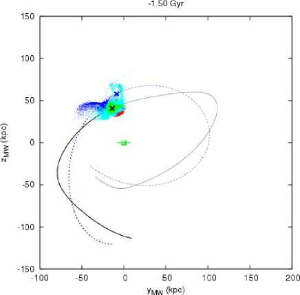
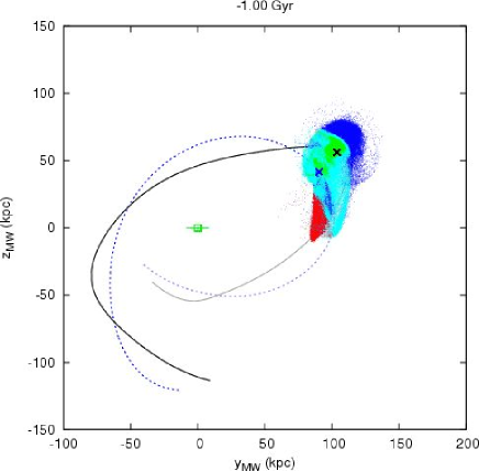
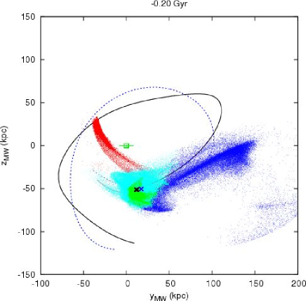
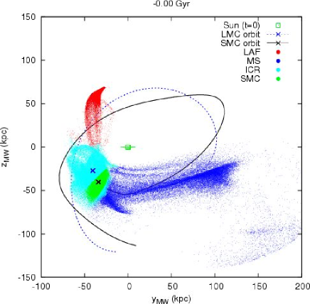
Figure 3: The particle configuration in the Galactocentric coordinate system at different timesteps. Different colour dots represent the particles which end up in different components at $T=0$ as shown in the bottom-right plot. See the text and Fig. 4 for the definitions of the MS, LAF, ICR, and SMC.

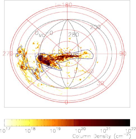
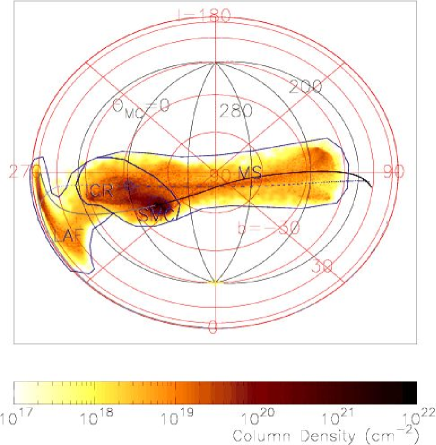
Figure 4: H i column density map (i.e. zeroth moment map) of the empirical data (left) and our fiducial model (right). A full sky Zenith Equal Area projection centred on the South Galactic Pole is applied, to preserve flux. Blue lines delineate regions used to quantify masses in Section 3.2. In the right panel, the enclosed regions with labels of MS, LAF, ICR, and SMC are arbitrarily chosen, and are used in Fig. 3. The current positions of the SMC and LMC are represented by black and blue ellipses, and in the right panel, the past and future $1{\rm\,Gyr}$ histories of the SMC and LMC orbit are denoted by black (solid) and blue (dashed) lines, respectively (the future $1{\rm\,Gyr}$ is shaded in a lighter colour). Lines of constant Magellanic Longitude are drawn in black, with the LMC lying on the $0\degr$ meridian.

3 Fiducial Model

In this section, we show the results of our fiducial model, the basic parameters for which are listed in Section 2 and Table 3. Since we are primarily interested in the formation of the MS and LAF, which we assume are both stripped H i gas components from the SMC disc, our analysis focuses on the particles which were initially within the original SMC disc. In what follows, our simulation products are compared closely with the empirical HIPASS dataset.

3.1 Evolution

In Fig. 3, we present a series of snapshots in the Galactocentric coordinate system, with the orbit of the MCs overlayed. Consistent with earlier models (e.g. GN96; YN03), when the SMC experienced a close encounter with the MW and the SMC $\sim 1.5{\rm\,Gyr}$ ago, the edge of the disc of the SMC began to be drawn out, which formed the tidal features that later became the LAF and MS. By $T=-1.0{\rm\,Gyr}$, at the subsequent apo-Galacticon, the LAF becomes more prominent, whilst the MS was still under development. By $T=-0.3{\rm\,Gyr}$, much of the initially stripped material in the leading tidal arm had been pulled back into the inter-cloud region (ICR), and the material still in the LAF was brought within $3{\rm\,kpc}$ of the solar circle. By this time, the MS and LAF morphology resemble that seen today. The next encounter with the MW and SMC at $T=-0.2{\rm\,Gyr}$ caused little obvious consequence to either the MS or LAF. It did however, cause the dispersion of much of the material that had been within the SMC. Much of this material either ended up in the ICR (although most of the ICR material was already in an ICR structure before this event), or contributed to the large spread in radial extent of the SMC. At the current time, the ICR extends radially from $\sim 30$ to $\sim 80{\rm\,kpc}$, and the SMC from $\sim 45$ to $\sim 60{\rm\,kpc}$.

We also ran the simulation “forward” in time to $T=+0.25{\rm\,Gyr}$ and found that the ICR undergoes mass loss with material being dragged out into two tidal tails, separated radially and kinematically from the main MS and LAF features. This is consistent with what is expected by Brüns et al. (2005). By $T=+0.25{\rm\,Gyr}$, the material in the ICR has been dragged $55{\rm\,kpc}$ towards the MS in the plane of the sky, giving an angular separation of $35\degr$ between the SMC and tip of the ICR.

3.2 H i column density distribution

In this section, we compare the present-day H i column density distribution between the empirical HIPASS dataset (Putman et al., 1998) and our simulation results. Fig. 4 displays the H i column density map on a Zenith Equal Area (ZEA) projection. Here, we arbitrarily define the regions corresponding to the MS, LAF, ICR, and SMC as shown in the right panel of Fig. 4. We converted the observed 21cm flux to H i column density, after Barnes et al. (2001). To construct H i column density maps from the simulation results, we assume that the disc particles in the SMC are purely gaseous, and the H i mass fraction is 0.76. The column densities within the SMC and ICR region will be somewhat overestimated, as we neglect currently any associated stellar and ionised components. On the other hand, Fig. 5 demonstrates that most particles in the MS and the LAF at $T=0$ originate in the outer edge of the initial SMC disc, where there was likely a lack of stars. To date, searches for a putative stellar component to the MS have proven unsuccessful (e.g. Philip, 1976b, a; Recillas-Cruz, 1982; Brueck & Hawkins, 1983). Regardless, the H i fraction of 0.76 remains technically an upper limit, and thus our predictions should considered as upper limits. For these reasons the comparisons between the simulation and the HIPASS data focus mainly upon the properties of the MS and LAF.

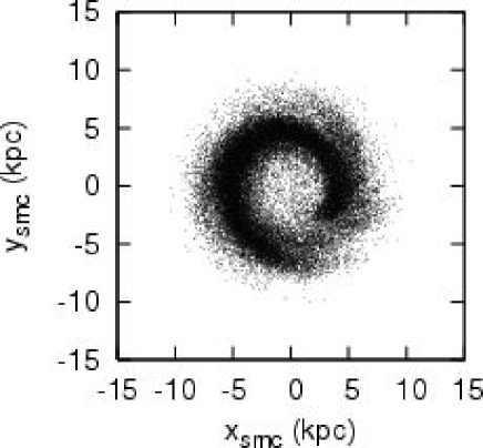
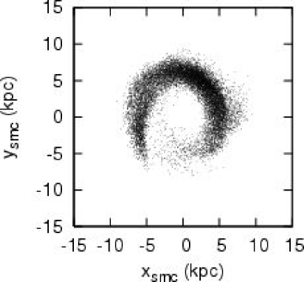
Figure 5: The distribution of the particles which end up in the MS (left) and LAF (right) at $T=0$ in the face-on view of the initial ($T=-2.5{\rm\,Gyr}$) SMC disc. For the definition of the MS and LAF see Fig. 4.

Fig. 4 shows that in our fiducial model the gross features of the observed MS are reproduced, and the LAF appears as a consequence of tidal interactions. This confirms previous studies, such as GN96 and YN03, which suggested that the MS and LAF features originate from gas stripped from the SMC disc by the tidal interaction with the LMC and MW.

The left panel of Fig. 7, itself a new representation of the HIPASS dataset, demonstrates that the observed leading arm extends above the Galactic plane to latitude $b\sim 30\degr$. While the full extent of the LAF above the plane remains a matter of debate (e.g. Brüns et al., 2005), the metallicity of its gas is consistent with an SMC origin (Lu et al., 1998; Gibson et al., 2000), supporting the tidal disruption scenario for the MS (and LAF). Furthermore, the observed H i cloud distribution seems to show “a kink” near $(l,b)=(310\degr,0\degr)$, where two further components of the LAF are seen north of the Galactic plane (labelled LAF II and III in Brüns et al., 2005). Although the exact position of the kink is inconsistent with the empirical data, our simulation does naturally predict its existence.

The tail of the observed MS shows spatial bifurcation near $(l,b)=(300\degr,-70\degr)$ and $(l,b)=(80\degr,-55\degr)$ in Fig. 4, with the two components forming an apparent twisting double helix-like structure (Putman et al., 2003). This bifurcation is not apparent in previous studies such as GN96 and YN03; higher resolution simulations enable us to study such subtle features. Since this might be further evidence of the tidal interaction between the LMC and SMC, we return to this issue later.

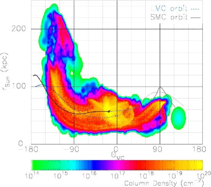
Figure 6: The heliocentric distance, as a function of the Magellanic longitude, derived from our fiducial model. The black (solid) and blue (dashed) lines show the past and future $1{\rm\,Gyr}$ histories (the future $1{\rm\,Gyr}$ is shaded a lighter colour) of distance and Magellanic longitude for the SMC and LMC, respectively.

An advantage of the present work is that the H i data available to constrain the models are significantly improved beyond that of GN96 or YN03. As in those previous studies, while the gross features of the observed MS and LAF are reproduced by our fiducial model, there remain subtle discrepancies between simulations and data. While the simulated MS is both broader and more extended than that observed (and hence the mean column density is somewhat lower than that encountered in the HIPASS dataset), the derived H i gas mass (assuming a heliocentric distance of $57{\rm\,kpc}$) from HIPASS is within 50 per cent of that of our simulated fiducial model ($3.5\times 10^{8}{\rm\,M}_{\sun}$ and $2.4\times 10^{8}{\rm\,M}_{\sun}$, respectively). Fig. 6 shows the heliocentric distance of the simulated MS and LAF against the Magellanic longitude, ${\theta}_{\rm MC}$ (as defined in Wakker, 2001; lines of constant ${\theta}_{\rm MC}$ are shown in Fig. 4). This demonstrates that the distance to the simulated MS is not constant, instead increasing across its length. Hence negating the distance ambiguity by obtaining a total flux gives us a fairer comparison than a total mass. Doing so results in an observed MS total H i flux of $4.8\times 10^{5}{\rm\,Jy\,{\rm\,km\,s}^{-1}{}}$, while the fiducial simulated MS has a total H i flux of $2.3\times 10^{5}{\rm\,Jy\,{\rm\,km\,s}^{-1}{}}$, still within a factor of $\sim 2$ of the HIPASS data.

Conversely, the simulated LAF has a predicted H i mass and associated flux ($7.3\times 10^{7}{\rm\,M}_{\sun}$ and $7.9\times 10^{4}{\rm\,Jy\,{\rm\,km\,s}^{-1}{}}$, respectively) both factors of $\sim$2 greater than that inferred from the HIPASS dataset ($3.5\times 10^{7}{\rm\,M}_{\sun}$ and $4.6\times 10^{4}{\rm\,Jy\,{\rm\,km\,s}^{-1}{}}$, respectively). One clear difference between observation and simulation is that of the geometry of the LAF, in particular that of the projected deflection angle between the LAF and a Great Circle aligned with the MS proper (Fig. 7). In addition, the simulated LAF extends above the Galactic Plane beyond that observed. We will discuss possible solutions to these apparent problems in Section 5.

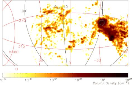
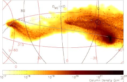
Figure 7: H i column density map of the LAF region derived from the HIPASS dataset (left) and that of our fiducial model (right) with ZEA projection centred on the LAF. The future orbits of the MCs are denoted by a lighter shading, demonstrating the similarity between the orbit of both MCs and the orbit of the LAF.

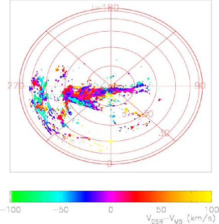
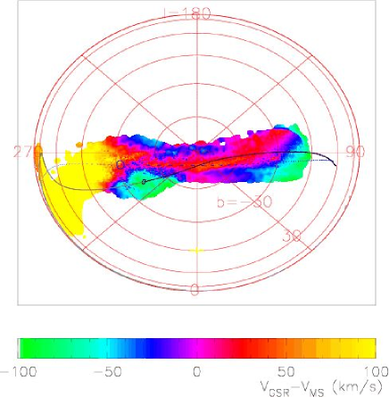
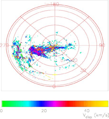
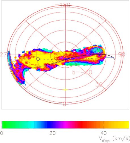
Figure 8: First (upper) and second (lower) moment maps derived from the HIPASS dataset (left) and that of our fiducial model (right).

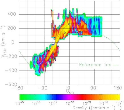
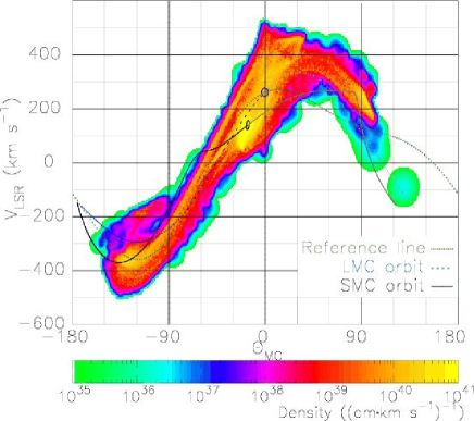
Figure 9: The line-of-sight velocity with respect to the Local Standard of Rest ${v}_{\rm LSR}$, as a function of the Magellanic longitude ${\theta}_{\rm MC}$, derived from the observed HIPASS dataset and that of our fiducial model. The black (solid) and blue (dashed) lines show the past and future $1{\rm\,Gyr}$ histories (the future $1{\rm\,Gyr}$ is shaded a lighter colour) of ${v}_{\rm LSR}$ and ${\theta}_{\rm MC}$ (where the longitude is defined with respect to the current position of the LMC) for the SMC and LMC, respectively. A reference line (dotted green) is drawn to show the velocity subtracted equally to yield the top panels of Fig. 8—see text for details.

3.3 H i kinematics

Fig. 8 shows the first and second moment maps for both our fiducial simulation and that derived from the HIPASS dataset. In order to remove the large velocity gradient along the MS (which acts to obscure fine kinematical details within the maps), the first moment map is shown as the distribution of the velocity of ${v}_{\rm GSR}-{v}_{\rm MS}$, where ${v}_{\rm MS}$ is the mean trend of velocity across the observed MS and LAF, and is defined in terms of two fitted Fourier components, ${v}_{\rm MS}=86\sin({\theta}_{\rm MC}+2.5\degr)-92\sin(2({\theta}_{\rm MC}-26.3\degr))$. The second moment map is the distribution of the velocity dispersion of H i gas.

In the first moment map, the observed velocity trend along our simulated MS is shown to be globally consistent with that of the empirical data. Fig. 9 displays ${v}_{\rm LSR}$ against the Magellanic longitude, ${\theta}_{\rm MC}$, and demonstrates perhaps more clearly that the mean velocity of the simulated MS is consistent with that observed. In contrast, the line-of-sight velocity of the simulated LAF is significantly larger than that observed, although it does follow the general trend of decreasing velocity at ${\theta}_{\rm MC}\ga 0$.

The second moment maps seen in the lower panels in Fig. 8 indicate that the velocity dispersion of the simulated LAF is roughly consistent with, although slightly higher, than that observed. However, the velocity dispersion of the simulated MS is somewhat greater than that inferred from the HIPASS dataset. This might be due to the neglect of gas dissipation via radiative cooling in the current suite of simulations, as will be examined further in Paper II.

We end by drawing attention to the evidence of a bifurcation in ${v}_{\rm LSR}$ (right panel of Fig. 9) within the MS and LAF. The next section discusses this bifurcation in more detail.

3.4 Spatial and velocity bifurcation

Our fiducial model shows a bifurcation in the MS, as seen in the ZEA spatial distribution of the H i column density of Fig. 4. Within the simulation, this bifurcation occurs both radially and tangentially. Fig. 4 displays the tangential bifurcation, and shows that there are two stream components that appear to follow a twisting topology governed by the orbits of the MCs – both the orbits and the bifurcation seem to cross at $(l,b)\sim(45\degr,-80\degr)$. Radially, the head of the Stream, just behind the MCs, has two components (Figs. 3 and 6). At the tail of the MS, there is a third component, well separated from the other two streams — extending from $170$ to $220{\rm\,kpc}$. It is visible only through its heliocentric distance from the Sun, and coincides with the $(l,b)$ position of the tip of the main streams. Also apparent in Figs. 6 and 7, are the radial and tangential bifurcations of the LAF, respectively.

The right panel of Fig. 9 demonstrates that the bifurcation of the MS appears also in ${v}_{\rm LSR}$. Plotted in Fig. 9 are lines showing the history (and future) of the MC’s ${v}_{\rm LSR}$. Only one of the bifurcated components follows the orbit of the Clouds (primarily the LMC), while the other possesses a higher velocity. Interestingly, there is a second velocity component at the position of the SMC (as well as at the head of the MS and the LAF). We remind the reader that Mathewson & Ford (1984) observed two velocity components within the SMC itself, with a separation of $\sim 50{\rm\,km\,s}^{-1}$. While the separation of our two velocity components is much larger, it might indicate that the two observed velocity components are caused by a similar process.

Snapshots of the simulation, similar to those seen in Fig. 3, hint at the origin of these bifurcations. Prior to the first major peri-Galacticon at $T=-1.5{\rm\,Gyr}$, an encounter with the LMC at $T=-2.2{\rm\,Gyr}$ drew the particles from the tip of the SMC disc closest to the LMC (and furthest from the MW), which resulted in the particles that eventually came to reside in the most distant MS component, at a Galactocentric distance of $170$ to $220{\rm\,kpc}$. The MS particles did not become “distinct” from the SMC proper until $T=-1.5{\rm\,Gyr}$; at $T=-1.05{\rm\,Gyr}$, the MS then received an impulse from an LMC encounter, which caused the spatial bifurcation of the MS. The MS was then given a “kick” by the LMC at the subsequent apo-Galacticon at $T=-0.55{\rm\,Gyr}$. This encounter at $T=-0.55{\rm\,Gyr}$ resulted in the MS being broken into two kinematic components, resulting in the apparent velocity bifurcation.

On the other hand, a portion of the LAF comes from the particles on the same side of the disc, but closer to the SMC centre at the $T=-2.2{\rm\,Gyr}$ encounter. The opposite side of the edge of the disc mostly consisted of particles that end up at the current time in the ICR. At $T=-0.9{\rm\,Gyr}$, the LMC passed through the LAF, splitting it into two bifurcated radial components.

Our models seem to create naturally both spatial and velocity bifurcations, via tidal interaction between the LMC and SMC. If this is the case, any observed bifurcation features would be strong evidence supporting the tidal formation scenario for the MS. Observationally, the left panel of Fig. 4 shows that there is spatial bifurcation in the observed H i distribution. However, from this data alone, it is difficult to ascertain from the ${v}_{\rm LSR}$ distribution of Fig. 9 whether there is an observed velocity bifurcation. Nevertheless, both Fig. 9 of this work, and Brüns et al. (2005), with data of higher velocity resolution, show evidence for a bifurcation in ${v}_{\rm LSR}$ along the MS, with the two components observed in this work being separated by approximately $100{\rm\,km\,s}^{-1}$ at ${\theta}_{\rm MC}\sim 100\degr$, and two components being visible in fig. 3 of Brüns et al. (2005) between the interface region and Galactic Plane. There is also a hint of bifurcation (with separation of $\sim 100{\rm\,km\,s}^{-1}$) in the LAF at ${\theta}_{\rm MC}\sim 45\degr$. Unfortunately, the current quality of the observational data is not enough to lead to a firm conclusion. Higher quality data cubes with improved velocity resolution will provide critical information concerning this apparent bifurcated structure.

4 Parameter Dependences

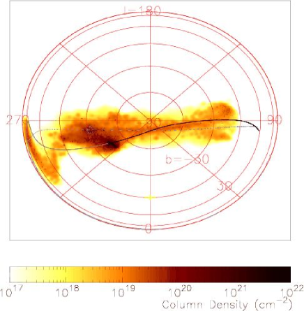
Figure 10: H i column density map for the lower-resolution simulation with the same parameter set as the fiducial model.

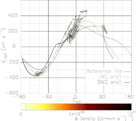
Figure 11: H i flux excess in the ${v}_{\rm LSR}$ vs. ${\theta}_{\rm MC}$ plane, for the high-resolution model over the low-resolution model, demonstrating the finer features visible. Contours are plotted at $5\times 10^{39}$ and $5\times 10^{40}({\rm cm}{\rm\,km\,s}^{-1})^{-1}$.

As explained in Section 2, our simulations involve several parameters which are not well-constrained by current observations. In this section, we briefly demonstrate how the final configurations of the MS and LAF are sensitive to these free parameters. We varied parameters over a wide range of parameter space in our survey, to obtain our fiducial model. The parameter survey was performed at a lower resolution (25,000 disc and 25,000 halo particles) than the final fiducial model. We have confirmed that in the fiducial model the results of the lower-resolution simulation are consistent with the higher-resolution simulation, although, as presented above, the choice of a higher resolution enables us to discuss more detailed features. For example, in Fig. 10, we show the H i column density map for the lower-resolution model with identical parameters as our fiducial model. The distribution of the H i column density is roughly consistent with that shown in Fig. 4, although the higher-resolution models affords an improved examination of the finer-scale structures intrinsic to the simulated streams. The bifurcation alluded to in the previous section is an example of such a feature, and is perhaps best appreciated through an inspection of Fig. 11, where the flux “excess” of the high-resolution model with respect to the lower-resolution model is presented in the ${v}_{\rm LSR}$ vs. ${\theta}_{\rm MC}$ plane, and the bifurcation becomes becomes readily apparent.

Most of the parameter space surveyed is summarised in Table 3. The scale height of the SMC disc, the ratio of SMC disc mass (H i mass in Table 3) to SMC halo (DM) mass, the velocity dispersion of the SMC disc, and the initial and final total mass of the SMC (varying the mass of the SMC for the purposes of the orbit calculation) were found not to be important to the evolution of the system. Both the velocity dispersion, and the ratio of H i to DM mass of the disc, simply scale the velocity dispersion and quantity of H i found in the final Streams and Clouds in a linear fashion.

In the parameter survey, the orbits of the MW, LMC and SMC were derived assuming the mass of the SMC is constant. However, we found that the SMC bound mass decreases from $3\times 10^{9}$ to $1.5\times 10^{9}{\rm\,M}_{\sun}$ approximately linearly with time between $T=-2.25{\rm\,Gyr}$ (near the first interaction between the LMC and SMC), and $T=0$. Such mass-loss may affect the orbit and the final features of the MS and LAF (e.g. Zhao, 2004; Knebe et al., 2005). Thus, we explore the effects of decreasing the mass of the SMC linearly with time from $3.0\times 10^{9}$ to $1.5\times 10^{9}{\rm\,M}_{\sun}$. We found that there is little change to the orbits, since the LMC, rather than the less massive SMC, primarily determines the orbit of both bodies in equations (4) and (5). As a result, we confirmed that the final features of the MS and the LAF are also not influenced heavily by the time evolution of the SMC mass. Thus, in all other simulations in the parameter survey, we use the orbits predicted with no evolution of the SMC mass. We now highlight the influence of the most important input parameters.

4.1 The initial scale length of the SMC disc

We found that the final H i distributions are sensitive to the scale length of the initial SMC disc. Fig. 12 shows the column density map of a model with a smaller scale length ($1.4{\rm\,kpc}$) for the initial SMC disc. This reduced scale length results in a lower total H i flux for the MS, as the initially more concentrated SMC mass distribution results in less material being stripped from the disc. Since the fiducial model does not have a total H i flux high enough to match perfectly the observations (Section 3.2), we conclude that reducing the SMC scale length is not appropriate. It is also worth noting that the smaller scale length model leads to a less significant bifurcation in the simulated MS.

To quantify the difference between the models, we have measured the H i masses and total fluxes within the regions delineated as the MS in Fig. 4. As a result, the low-resolution simulation of the fiducial model has an H i mass in the MS of $2.4\times 10^{8}{\rm\,M}_{\sun}$ and total H i flux of $2.5\times 10^{5}{\rm\,Jy\,{\rm\,km\,s}^{-1}{}}$. The low-resolution simulation has a very similar mass to that of the high-resolution case (see Section 3.2). On the other hand, the small scale length model leads to a MS H i mass and total flux of $1.8\times 10^{8}{\rm\,M}_{\sun}$ and $1.9\times 10^{5}{\rm\,Jy\,{\rm\,km\,s}^{-1}{}}$ respectively, which is significantly smaller than that of the fiducial model. Since the fiducial model has a mass which is somewhat lower than that inferred from the HIPASS dataset, we again conclude that the models derived with the reduced initial scale length for the SMC perform worse than the fiducial selection.

The H i survey of late-type dwarf galaxies by Swaters et al. (2002) suggested that the range of scale lengths of the gas disc for galaxies which have a similar H i mass to that of the SMC is 1.5 – $4.5{\rm\,kpc}$. The scale length of our fiducial model ($3.5{\rm\,kpc}$) appears reasonable, and thus the progenitor of the SMC is considered to have had a large H i disc before the SMC fell towards the MW.

We note that choosing a smaller scale radius is similar to setting a small truncation radius, in that the SMC material is concentrated more strongly towards the centre of the SMC, where it is more difficult to tidally strip. We obtain similar results to the above when we choose smaller SMC truncation radii, such that the stream is substantially retarded when the truncation radius is reduced from $7{\rm\,kpc}$ to $4{\rm\,kpc}$. In this situation, the MS H i mass and total flux are reduced to $7.2\times 10^{7}{\rm\,M}_{\sun}$ and $7.0\times 10^{4}{\rm\,Jy\,{\rm\,km\,s}^{-1}{}}$. The LAF mass is scaled in a similar manner in both cases.

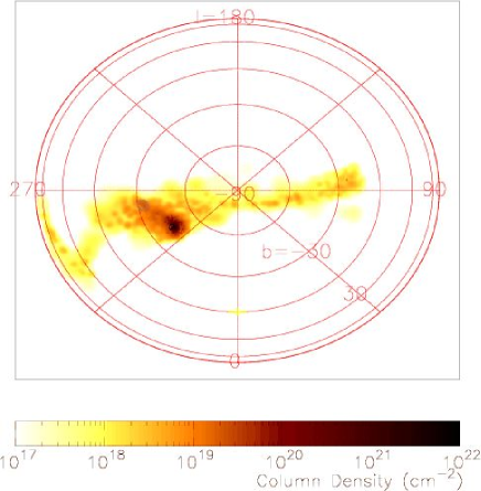
Figure 12: H i column density map for models with a smaller scale length ($1.4{\rm\,kpc}$) for the initial SMC disc.

4.2 The inclination angle of the SMC

As mentioned in Section 2.3, the current inclination angle of the SMC is unknown, and the initial disc angle $\theta$ and $\phi$ are free parameters in our simulations. Fig. 13 shows the H i column density distribution for the models with $(\theta,\phi)=(30\degr,210\degr)$ and $(45\degr,230\degr)$, to demonstrate how these angles affect the final distribution of the MS and LAF. We remind the reader that we use $(\theta,\phi)=(45\degr,210\degr)$ in the fiducial model, and therefore small differences of only $20\degr$ in the initial inclination angle have quite a marked effect on the details of the final distribution. If accurate observations of the current inclination angle of the SMC were to be made, it would provide a strong constraint on any putative model of the formation of the MS.

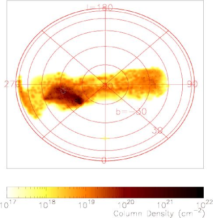
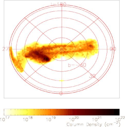
Figure 13: H i column density map for the model $(\theta,\phi)=(30\degr,210\degr)$ (left) and $(45\degr,230\degr)$ (right). The current positions of the SMC and LMC are represented by a black ellipse (the ellipse is the projection of the SMC disc at the given angle) and blue circle respectively.

4.3 The mass of the LMC

Another unknown parameter is that of the mass of the LMC itself. At the time of the GN96 study, the mass of the LMC was believed to be $\sim 2\times 10^{10}{\rm\,M}_{\sun}$ (e.g. Schommer et al., 1992). However, recently, some authors claim the lower mass of the LMC (e.g. van der Marel et al., 2002 who suggested that the mass of the LMC within $R<8.9{\rm\,kpc}$ is about $9\times 10^{9}{\rm\,M}_{\sun}$). Motivated by such claims, we also ran models with varying orbital parameters, and in particular, a lower LMC mass. Fig. 14 shows the result of a model with an LMC mass of $1.5\times 10^{10}{\rm\,M}_{\sun}$. Even such small differences in the LMC mass cause a large change in the orbits of the LMC and SMC. Since the MS follows the past orbit of the MCs, the angle of the MS is radically different between the model with small LMC mass, and both the fiducial model and the observed MS. This result suggests that such a low mass LMC is unlikely, if the MS is the result of tidal interactions.

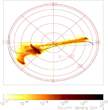
Figure 14: H i column density map for the model with an lower LMC mass of $1.5\times 10^{10}{\rm\,M}_{\sun}$. The past and future $1{\rm\,Gyr}$ histories of the orbit resulting from this differing LMC mass are presented by black solid and blue dashed lines for the SMC and LMC respectively.

5 Summary and Discussions

We have carried out high-resolution N-body simulations of the history of the SMC disturbed by tidal interactions with the MW and LMC. We have surveyed most of the possible parameter space for the SMC orbit and the properties of the initial SMC disc, and found the best model. The increased numerical resolution of $\sim 7{\rm\,Jy\,{\rm\,km\,s}^{-1}{}}$ per particle for the H i flux, $\sim 30$ times higher than the previous studies (GN96; G99; YN03), made it possible for us to examine the detailed features of both leading and trailing tidal streams. Taking advantage of this higher resolution, we for the first time made a direct and quantitative comparison of the simulation results with newly available high quality observational data from HIPASS. We convolved the HIPASS dataset with the identical software tools used to analyse the simulated datasets, and compared the results in identical manners. Such comparisons confirm the conclusions of previous studies – that the existence of the LAF and MS can be explained by the leading and trailing streams of the SMC created by tidal interactions with the MW and LMC. However, our quantitative comparison have revealed extant problems with the models (some minor; some more significant). We found that even in our best model (1) the shape of the MS is too extended in both width and length (Section 3.2); (2) the total H i flux of the MS is too low, and thus the mass of the MS is too low (Section 3.2); (3) the angle the LAF emanates from the MCs is not entirely consistent with observations (Section 3.2); (4) and nor is its total H i flux consistent with observations (Section 3.2); (5) the velocity dispersion of the MS is too high (Section 3.3); and (6) the line of sight velocity of the LAF is too high (Section 3.3).

These problems suggest that additional physics may be required to explain the observed properties of the MS and LAF, quantitatively. Obvious physics which this study excludes are gas physics, such as hydrodynamics and dissipation by radiative cooling. Simulations in Maddison et al. (2002) indicate that dissipation causes the MS to become narrower, which might lead to a reduced velocity dispersion. Ram pressure (Moore & Davis, 1994; Mastropietro et al., 2005) is another physical process which our numerical model does not currently take into account. Ram pressure (or drag – see Gardiner, 1999) is expected to shorten the leading arm and increase the gas density in the MS, which should help to solve the deficiencies of the model at recreating the LAF and MS with their correct shapes and densities. If it were to also bring the MS significantly closer than the $57{\rm\,kpc}$ fixed for the observational data within this paper, then the mass of the observed stream and total flux of the modelled stream would be increased, bringing them back into agreement. However, drag might lead to more problems for the length of the MS. Another possibly important mechanism is supernovae feedback which might aid in ejecting gas from the SMC and/or LMC, and help to increase the gas density in the MS and LAF. Finally, we note that the LAF passed very close to the centre of the MW $0.2{\rm\,Gyr}$ ago, and since we modelled the MW potential as spherically symmetric with a constant rotational velocity of $220{\rm\,km\,s}^{-1}$, any deviations from this (such as the unknown contribution from the MW disc; e.g. Fich & Tremaine, 1991) would affect our modelled LAF in particular. We are in the midst of introducing these physical processes into our simulations, and will report upon their respective effects in Paper II.

Another benefit of the higher-resolution simulations performed here is the identification of the bifurcation of the MS and LAF both spatially and kinematically. Our simulations predict that if the MS is created by a tidal interaction with the LMC, the bifurcation would appear both in the H i column density map and the line-of-sight velocity versus Magellanic longitude plane. Current observations are consistent with the existence of a spatial bifurcation in the H i column density map (left panel of Fig. 4). In the velocity versus Magellanic longitude plane, it is difficult to make a firm conclusion from the current HIPASS data, although it is interesting that the SMC itself is found to consist of at least two velocity components (Mathewson & Ford, 1984), perhaps caused by the same tidal disruption processes that form the bifurcation in our models. Observations with high velocity resolution and sensitivity may be able to test our prediction of bifurcation within the MS. If confirmed, it would provide strong evidence that the MS was created by tidal interactions.

References

- Barnes et al. (2001) Barnes D. G., et al., 2001, MNRAS, 322, 486
- Bekki & Chiba (2005) Bekki K., Chiba M., 2005, MNRAS, 356, 680
- Bekki et al. (2004) Bekki K., Couch W. J., Beasley M. A., Forbes D. A., Chiba M., Da Costa G. S., 2004, ApJ, 610, L93
- Binney & Tremaine (1987) Binney J., Tremaine S., 1987, Galactic dynamics. Princeton, NJ, Princeton University Press, 1987, 747 p.
- Brüns et al. (2005) Brüns C., et al., 2005, A&A, 432, 45
- Brueck & Hawkins (1983) Brueck M. T., Hawkins M. R. S., 1983, A&A, 124, 216
- Dopita et al. (1985) Dopita M. A., Lawrence C. J., Ford H. C., Webster B. L., 1985, ApJ, 296, 390
- Faber & Lin (1983) Faber S. M., Lin D. N. C., 1983, ApJ, 266, L17
- Feast & Walker (1987) Feast M. W., Walker A. R., 1987, ARA&A, 25, 345
- Fich & Tremaine (1991) Fich M., Tremaine S., 1991, ARA&A, 29, 409
- Gardiner (1999) Gardiner L. T., 1999, in Astronomical Society of the Pacific Conference Series N-body Simulations of the Magellanic Stream. pp 292–+
- Gardiner & Noguchi (1996) Gardiner L. T., Noguchi M., 1996, MNRAS, 278, 191
- Gardiner et al. (1994) Gardiner L. T., Sawa T., Fujimoto M., 1994, MNRAS, 266, 567
- Gibson et al. (2000) Gibson B. K., Giroux M. L., Penton S. V., Putman M. E., Stocke J. T., Shull J. M., 2000, AJ, 120, 1830
- Hardy et al. (1989) Hardy E., Suntzeff N. B., Azzopardi M., 1989, ApJ, 344, 210
- Hashimoto et al. (2003) Hashimoto Y., Funato Y., Makino J., 2003, ApJ, 582, 196
- Hatzidimitriou et al. (1997) Hatzidimitriou D., Croke B. F., Morgan D. H., Cannon R. D., 1997, A&AS, 122, 507
- Ibata et al. (1994) Ibata R. A., Gilmore G., Irwin M. J., 1994, Nature, 370, 194
- Just & Peñarrubia (2005) Just A., Peñarrubia J., 2005, A&A, 431, 861
- Kawata & Gibson (2003) Kawata D., Gibson B. K., 2003, MNRAS, 340, 908
- Knebe et al. (2005) Knebe A., Gill S. P. D., Kawata D., Gibson B. K., 2005, MNRAS, 357, L35
- Kuijken & Dubinski (1995) Kuijken K., Dubinski J., 1995, MNRAS, 277, 1341
- Lin et al. (1995) Lin D. N. C., Jones B. F., Klemola A. R., 1995, ApJ, 439, 652
- Lu et al. (1998) Lu L., Sargent W. L. W., Savage B. D., Wakker B. P., Sembach K. R., Oosterloo T. A., 1998, AJ, 115, 162
- Maddison et al. (2002) Maddison S. T., Kawata D., Gibson B. K., 2002, Ap&SS, 281, 421
- Martin et al. (2005) Martin N. F., Ibata R. A., Conn B. C., Lewis G. F., Bellazzini M., Irwin M. J., 2005, MNRAS, 362, 906
- Mastropietro et al. (2005) Mastropietro C., Moore B., Mayer L., Wadsley J., Stadel J., 2005, MNRAS, pp 835–+
- Mathewson et al. (1974) Mathewson D. S., Cleary M. N., Murray J. D., 1974, ApJ, 190, 291
- Mathewson & Ford (1984) Mathewson D. S., Ford V. L., 1984, in IAU Symp. 108: Structure and Evolution of the Magellanic Clouds H I surveys of the Magellanic System. pp 125–136
- Moore & Davis (1994) Moore B., Davis M., 1994, MNRAS, 270, 209
- Muller et al. (2003) Muller E., Staveley-Smith L., Zealey W., Stanimirović S., 2003, MNRAS, 339, 105
- Murai & Fujimoto (1980) Murai T., Fujimoto M., 1980, PASJ, 32, 581
- Murali et al. (2002) Murali C., Katz N., Hernquist L., Weinberg D. H., Davé R., 2002, ApJ, 571, 1
- Philip (1976a) Philip A. G. D., 1976a, BAAS, 8, 532
- Philip (1976b) Philip A. G. D., 1976b, BAAS, 8, 352
- Putman et al. (1998) Putman M. E., et al., 1998, Nature, 394, 752
- Putman et al. (2003) Putman M. E., Staveley-Smith L., Freeman K. C., Gibson B. K., Barnes D. G., 2003, ApJ, 586, 170
- Recillas-Cruz (1982) Recillas-Cruz E., 1982, MNRAS, 201, 473
- Schommer et al. (1992) Schommer R. A., Suntzeff N. B., Olszewski E. W., Harris H. C., 1992, AJ, 103, 447
- Stanimirović et al. (1999) Stanimirović S., Staveley-Smith L., Dickey J. M., Sault R. J., Snowden S. L., 1999, MNRAS, 302, 417
- Stanimirović et al. (2004) Stanimirović S., Staveley-Smith L., Jones P. A., 2004, ApJ, 604, 176
- Swaters et al. (2002) Swaters R. A., van Albada T. S., van der Hulst J. M., Sancisi R., 2002, A&A, 390, 829
- Tully (1988) Tully R. B., 1988, Nearby galaxies catalog. Cambridge and New York, Cambridge University Press, 1988, 221 p.
- van der Marel et al. (2002) van der Marel R. P., Alves D. R., Hardy E., Suntzeff N. B., 2002, AJ, 124, 2639
- Wakker (2001) Wakker B. P., 2001, ApJS, 136, 463
- Wakker & van Woerden (1991) Wakker B. P., van Woerden H., 1991, A&A, 250, 509
- Yoshizawa & Noguchi (2003) Yoshizawa A. M., Noguchi M., 2003, MNRAS, 339, 1135
- Zhao (2004) Zhao H., 2004, MNRAS, 351, 891