Observations and Modeling of the 2 – 25 $\micron$ Emission From High Mass Protostellar Object Candidates

Abstract

This is a report on detailed modeling of young high-mass protostellar candidates during their most embedded and obscured phases. We performed narrowband mid-infrared imaging of three candidate high-mass protostellar objects in G11.94-0.62, G29.96-0.02, and G45.07+0.13 at Gemini Observatory using the Thermal-Region Camera and Spectrograph (T-ReCS). The sources were imaged through up to 11 narrowband filters, sampling their SEDs over the entire 2–25 $\mu$m infrared range. For the first time, we have fit the observed SEDs of massive protostars with models that take into account departures from spherical symmetry in the infalling envelopes. In this way, we have been able to back out of the models detailed physical parameters for these earliest stages of massive stellar life. Our detailed modeling suggests that massive star formation can proceed in a way very similar to the formation of low-mass stars.

1 Introduction

The most massive stars begin their lives in the darkest recesses of giant molecular clouds, obscured from our view by a thick veil of dust and gas. Most of the time the earliest stages of massive star formation cannot be observed at visual wavelengths, and in many cases even the near-infrared emission from these protostars cannot escape. We owe much of our ignorance of the massive star formation process to the fact that we have a very limited range of wavelengths at our disposal with which to observe these youngest stages of massive stellar evolution.

The problem is further compounded by the fact that massive OB stars ($\geq$ 8 M_☉) are relatively few in number and, like all stages of massive stellar evolution, the formation process proceeds very quickly. It is therefore difficult to catch massive stars in the act of forming. Additionally, there is the problem of observing these objects with sufficient angular resolution. Massive star-forming regions generally lie at kiloparsec distances, making them more than an order of magnitude farther away than the closest low-mass star-forming regions. Furthermore, the percentage of binaries and multiple star systems increases as a function of mass (Larson 2001), and consequently it is believed that the vast majority of massive stars do not form alone. It is this combined distance and multiplicity problem that makes it difficult to resolve and study in detail a single massive star in its earliest years of formation.

Observations that have been extremely helpful in the study of massive stars have been cm-wavelength radio continuum and molecular line emission observations. Interferometric arrays can observe with subarcsecond angular resolution the radio continuum emission from the photoionized region in the near-stellar environment around young massive stars. These compact or ultra-compact H II (UC H II) regions are thought to exist $\sim$10⁵ years after the formation of a massive star (De Pree, Rodríguez, & Goss 1995). Until recently, this was the earliest observed phase of massive star formation.

In order to understand better their formation process, we need to observe massive stars at ages even younger than 10⁵ years. This means trying to observe sources before they develop UC H II regions, which in most of the cases limits our window of continuum observations to a relatively narrow wavelength regime from the mid-infrared ($\sim$3 $\mu$m) to the millimeter ($\sim$1 mm). Observing sources in this “high mass protostellar object” (HMPO) phase presents a challenge since the best resolutions achievable throughout most of this wavelength range (namely the far-infrared to the sub-millimeter) have, until recently, been on the order of a few to tens of arcseconds. However, the bright molecular line emission from these sources would still be observable with high angular resolution radio interferometers.

Hot cores of compact and dense molecular gas have been known to exist in massive star forming regions for several decades now (e.g., Wilson, Downes, & Bieging 1979). Some of these “hot molecular cores” (HMCs) are simply externally heated knots of material, but others may have stars forming at their centers. Recently some HMCs have been gaining serious attention as possibly forming extremely young massive stars at their centers (Cesaroni et al. 1994; Kurtz et al. 2000). Walmsley (1995) proposed that these types of HMCs are undergoing an intense accretion phase which prevents the development of a UC H II region. Since these types of HMCs do not possess radio continuum emission and are internally heated by massive protostars, they fit into the category of HMPOs.

Though the compositions of these sources are beginning to be understood in detail through the molecular line studies (e.g., Rodgers & Charnley 2001), continuum observations remain few because of the angular resolution problem. However, continuum observations from the mid-infrared to millimeter have the potential for revealing valuable information about the massive star formation process. Models of the spectral energy distribution (SED) of HMCs have been developed under the assumption that they have a central massive star undergoing spherical accretion of a free-falling envelope of dust and gas (Osorio, Lizano, & D’Alessio 1999). The success of these models in fitting the observable characteristics of HMCs gave strong support to the hypothesis that some of these objects were true HMPOs (i.e., not starless HMCs) in a stage previous to the development of an UC H II region. However, for that work, only mid-infrared upper limits were available in most of the sources. Since the mid-infrared range of the SED is highly sensitive to the geometry of the source (i.e., degree of flattening), in principle, these kinds of observations would allow testing of more sophisticated models, with a degree of detail similar to that of those that have been developed for low-mass protostars (e.g., Osorio et al. 2003).

Recently, observations by De Buizer (2004) and De Buizer et al. (2003) have identified four candidate HMPOs that have been observed in the mid-infrared with high-angular resolution. These HMPO candidates lie in areas of high mass star formation, as evidenced by nearby UC H II regions. In fact in two of these four cases, high spatial resolution observations from 8m telescopes were needed to simply isolate the mid-infrared emission of the HMPOs from the nearby UC H II regions. This means that, though more sensitive than what is achievable from the ground, data from infrared satellites like MSX ($\sim$5$\arcsec$ at 8 $\micron$, $\sim$13$\arcsec$ at 21 $\micron$), and even the Spitzer Space Telescope ($\sim$2$\arcsec$ at 8 $\micron$, $\sim$6$\arcsec$ at 24 $\micron$), are in general not adequate for these studies because of their relatively poor angular resolutions. By being able to isolate emission from the HMPO alone, mid-infrared observations from ground-based 8 to 10m-class telescopes represent a invaluable tool in the study of these earliest stages of massive star formation.

In this article we present new sub-arcsecond mid-infrared observations of three of the four candidate HMPOs identified by De Buizer (2004) and De Buizer et al. (2003). The fourth HMPO candidate, G305.20+0.21, will be the subject of a following article. Using the Gemini South telescope we imaged these three HMPO candidates through up to 11 filters, sampling their SEDs over the entire 2–25 $\mu$m infrared atmospheric window. Our motivation for performing these observations was to sample the SEDs of HMPOs with sufficient spectral resolution and coverage to accurately test new SED models. These models use envelopes that take into account deviations from spherical geometry in their inner region due to rotation and at large scales due to natural elongation of the source. By matching these models to the data we attempt to “back out” of the models detailed physical parameters for these earliest stages of massive stellar life. In this way, we hope to be able to learn some details about the massive star formation process during these highly obscured stages, as well as the strength and limitations of the non-spherical SED models.

2 Observations

Observations were carried out at Gemini South over the time period between 2003 September and 2004 November. Imaging was performed with the Thermal-Region Camera and Spectrograph (T-ReCS). The instrument employs a Raytheon 320$\times$240 pixel Si:As IBC array which is optimized for use in the 7–26 $\mu$m wavelength range, but can perform with modest sensitivity in the 2–5 $\mu$m wavelength range as well. The pixel scale is 0.089$\arcsec$/pixel, yielding a field of view of 28$\farcs$8$\times$21$\farcs$6. Sky and telescope subtraction were achieved through the standard chop-nod technique.

Images were performed with K, L, and M filters, as well as six narrowband silicate filters encompassing the full 10 $\mu$m N-band spectral window, and two narrowband filters within the 20 $\mu$m Q-band spectral window. Effective central wavelengths for these filters and their spectral range are given in Table 1. For G11.94-0.62 and G45.07+0.13 we also have images from De Buizer et al. (2003) through the Q3 ($\lambda_{o}$=20.81 $\mu$m, $\Delta\lambda$=19.99–21.64 $\mu$m) filter from the NASA Infrared Telescope Facility (IRTF) using the instrument MIRLIN.

Table 1 also lists the on-source integration times through each of the T-ReCS filters for each HMPO candidate field. In addition, this table lists the standard star used to flux calibrate each image, and the assumed flux density for that standard through the given filter. These assumed standard star flux densities were found by convolving the spectral irradiance templates of the stars from Cohen et al. (1999) with the given T-ReCS filter transmission profile.

Flux densities were derived for each filter for the HMPO candidate as well as any other mid-infrared sources on the field. Tables 2-4 list the flux densities for all sources. These flux densities are quoted with their 1-$\sigma$ total error, which is a quadrature addition of the statistical variation from the aperture photometry (due to the standard deviation of the background array noise) and the flux calibration error. Usually the flux calibration error is found from the variation of the standard star flux throughout the course of the night, however our observations were taken piece-wise on many nights throughout several semesters. Flux calibration was therefore achieved by observing a standard star at a similar airmass just before or after the observation of the target science field. Therefore, we do not have calibration variability statistics for each filter on each night the data were taken. However, the calibration factor [ratio of accepted flux in Janskys to analog-to-digital converter units (ADUs) per second per pixel] derived from the standard star observations through each filter varied little throughout 14 months of data collection, and so we use here the standard deviation of the calibration factor over this 14 month period as the flux calibration error. This can be considered an extremely conservative estimate of the errors, taking into account a wide variety of atmospheric and observing conditions that affect flux calibration. Most filters have modest flux calibration errors (for mid-infrared observations) with standard deviations between 2 and 10%. Flux calibration through certain filters is more difficult due to the presence of various atmospheric absorption lines contaminating the filter bandpass, some of which can be highly variable. Those filters most affected are the 7.7 $\mu$m (21%), 12.3 $\mu$m (19%), 18.3 $\mu$m (15%), and 24.6 $\mu$m (23%) filters.

Furthermore, the continuum observed through these filters may be affected by the presence of certain spectral features common to young stellar objects. In particular, the 12.3 $\mu$m continuum flux densities for the targets may be skewed to higher values due to the presence of bright [NeII] lines at 12.8 $\mu$m (see for instance, Faison et al. 1998). The 18.3 $\mu$m and 20.8 $\mu$m observations can also be skewed high or low depending on the presence in either emission or absorption of the 18 $\mu$m silicate feature.

3 The Targets

The three sources below were chosen because they are among the only HMPO candidates known to be bright in the mid-infrared (De Buizer 2004, De Buizer et al. 2003) and are sufficiently far enough away from nearby H II regions to be studied in detail without confusion. All three sources are thought to be HMPOs primarily because they are sources found in regions of known high mass star formation yet have no UC H II emission of their own, and all are coincident with molecular maser emission which is thought to trace massive star formation and its processes. Each source has further unique evidence indicating that it is a HMPO, which we discuss in detail below. A summary of the observations for each object will also be discussed in this context.

3.1 G11.94-0.62

Of the four sources identified as mid-infrared bright HMPO candidates by De Buizer (2004) and De Buizer et al. (2003), the status of the source in G11.94-0.62:DRT03 1 as a genuine HMPO is the most uncertain. However the HMPO candidate in G11.94-0.62 satisfies, at the very least, the minimum criteria outlined at the beginning of this section. DRT03 1 was found as an unresolved mid-infrared source in the survey of De Buizer et al. (2003) located at the site of a water maser clump offset $\sim$10$\arcsec$ from a cometary UC H II region. DRT03 1 has no detected cm radio continuum emission of its own.

However, G11.94-0.62 has not been observed with high spatial resolution molecular line imaging. Some molecular tracers have been discovered toward the region, like CS (Bronfman et al. 1996) and NH₃ (Cesaroni, Walmsley, & Churchwell 1992), but it is not known if this emission is related to the nearby UC H II region, the HMPO candidate, or both. While it is encouraging that some molecules have been found in the region, CH₃CN (a tracer of denser and hotter molecular material and indicator of the presence of HMCs) has been searched for in the region and was not detected (Watt & Mundy 1999). The UC H II region was also imaged at 2.7 mm by Watt & Mundy (1999), but there was no detection at the site of DRT03 1.

De Buizer et al. (2003) derive a lower limit to the bolometric luminosity for DRT03 1, finding that it is at least as bright as a B9 star. Though this spectral type is derived from an extreme lower limit to the bolometric luminosity, it does not appear that this source is a massive (M$>$10$M_{\odot}$) protostar, but more likely an intermediate mass protostellar object. If this is true, given its observational similarities to its higher mass counterparts, it will be interesting to study the similarities and differences in detail to learn more about the interrelation of the intermediate and high mass star formation processes. It would also have interesting consequences for the hypotheses regarding excitation of water masers by lower mass (non-ionizing) stars (Forster & Caswell 2000).

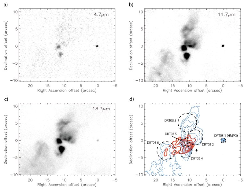
Figure 1: Images of the G11.94-0.62 field taken at a) 4.7 $\mu$m, b) 11.7 $\mu$m, and c) 18.3 $\mu$m at Gemini South with T-ReCS. d) A contour plot (smoothed by 0$\farcs$36) of the 11.7 $\mu$m image (blue contours) of the field showing sources with their labels and encircled with dashed lines that represent the apertures used for photometry. These aperture radii are given in the notes in Table 2. Plotted as crosses are the locations of the water maser groups as given by Hofner & Churchwell (1996). Also plotted (red contours) are the 2 cm radio continuum contours from Hofner & Churchwell (1996). The origin of each panel is the mid-infrared peak of the HMPO candidate (R.A.(J2000) = 18^h 14^m $00\hbox to0.0pt{.\hss}^{s}29$, Decl.(J2000) = $-18^{\circ}$ $53^{\prime}$ $23\farcs 1$).

Our sensitive Gemini mid-infrared observations of the region around G11.94-0.62 have revealed extended dust structure, the likes of which are not seen at any other spectral regime (Figure 1). These images at the sub-arcsecond angular resolution of Gemini confirm the results of the lower resolution observations of De Buizer et al. (2003) that the mid-infrared morphology of the UC H II region is not cometary, as is seen in cm radio continuum emission (Wood & Churchwell 1989). The HMPO candidate, DRT03 1, is clearly detected at shorter mid-infrared wavelengths but is only a 3-$\sigma$ and 4-$\sigma$ detection at 20.8 and 24.6 $\mu$m, respectively.

With no information on the Rayleigh-Jeans side of the SED for the HMPO candidate alone, we will not be able to constrain the models at the longer wavelengths. Table 2 lists the observed flux densities for the HMPO candidate as well as for the other mid-infrared sources in the field. It is not clear if each of these mid-infrared sources house a stellar component or if they are simply knots of dust in an extensive H II region.

3.2 G29.96$-$0.02

The HMPO candidate in G29.96$-$0.02 is sufficiently well-studied to be considered a prototype. The hot molecular component of this source was first discovered in the observations of Cesaroni et al. (1994). In this work, a hot (T_K$>$ 50 K) core of molecular material was detected, traced by NH₃(4,4) line emission near to, but offset $\sim$2$\arcsec$ from a cometary-shaped H II region. This hot molecular core was found to be coincident with a cluster of water masers. Cesaroni et al. (1994) conjectured that this source, like the other HMCs in their survey, is internally heated by a developing massive protostar. However, as was mentioned in the introduction, some HMCs could be externally heated by the nearby massive stars powering the UC H II regions. In the case of G29.96-0.02, the millimeter line study of Gibb, Wyrowski, & Mundy (2003) provided strong evidence that the HMC is internally heated. Therefore, the HMC in G29.96-0.02 appears to be a genuine HMPO.

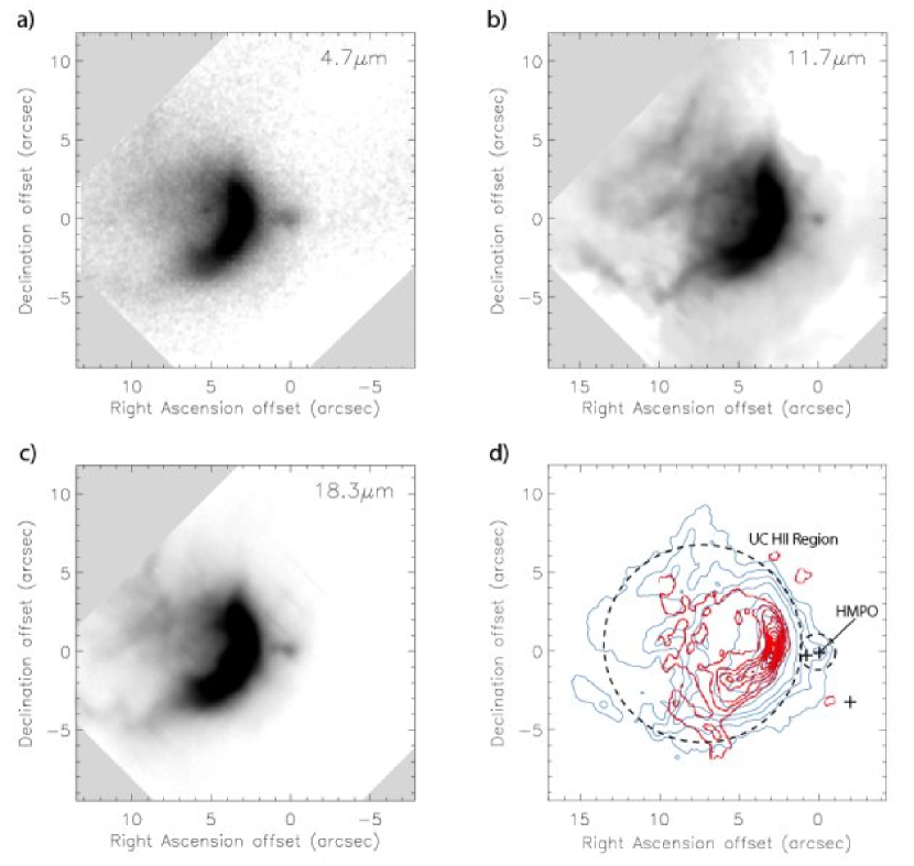
Figure 2: Images of the G29.96-0.02 field taken at a) 4.7 $\mu$m, b) 11.7 $\mu$m, and c) 18.3 $\mu$m at Gemini South with T-ReCS. These images had to be de-rotated to show north up and east left, hence the gray areas with no data in the corners of the panels. d) A contour plot (smoothed by 0$\farcs$18) of the 11.7 $\mu$m image (blue contours) of the field showing sources with their labels and encircled with dashed lines that represent the apertures used for photometry. These aperture radii are given in the notes in Table 3. Plotted as crosses are the locations of the water maser groups as given by Hofner & Churchwell (1996). Also plotted (red contours) are the 2 cm radio continuum contours from Hofner & Churchwell (1996). The origin of each panel is the mid-infrared peak of the HMPO candidate (R.A.(J2000) = 18^h 46^m $03\hbox to0.0pt{.\hss}^{s}74$, Decl.(J2000) = $-02^{\circ}$ $39^{\prime}$ $22\farcs 1$).

The HMPO in G29.96-0.02 was directly imaged for the first time in the mid-infrared by De Buizer et al. (2002) on the Gemini North 8-m telescope. The HMPO lies $\sim$3$\arcsec$ away from the radio continuum peak of the bright H II region and the emission from the UC H II region peak cannot be resolved from the HMPO on 4-m class telescopes (Watson et al. 2003). However, the large aperture of Gemini has sufficient resolving power in the mid-infrared ($\sim$0$\farcs$5) to pull in the peak of the dust emission from the H II region to allow direct observation of the HMPO. Even so, the resolved thermal dust emission from the H II region is still extensive, and therefore we cannot avoid observing the HMPO overlaid on a diffuse background of emission (Figure 2). Following the technique outlined by De Buizer et al. (2002), one can fit this background emission and subtract it off, effectively leaving only the mid-infrared emission of the HMPO. This technique was employed for the images obtained in the work presented here. In Table 3 we present the flux densities for the HMPO candidates and the UC H II, as well as the flux density of the HMPO candidate without subtracting off the background due to the extended UC H II emission. This was done so that it is transparent to the reader how much flux has been subtracted off, and what the absolute upper limits are for the flux densities of the HMPO candidate.

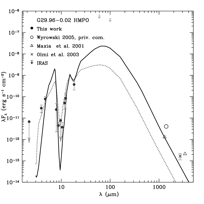
Figure 6: Observed and model SEDs for the source G29.96-0.02 HMPO. The different symbols represent the observed values of the flux density. Error bars are 3-$\sigma$ for the IR data. The 2.7 mm error bars correspond to the uncertainties assigned by Olmi et al. 2003 due to the subtraction method employed. No errors are available for the remaining millimeter flux densities. Upper limits are represented by arrows. Solid line represents the best fit model, obtained with $i=12^{\circ}$, $R_{c}=570$ AU, $L_{*}=1.8\times 10^{4}~{}L_{\odot}$, and $\rho_{\rm 1\,AU}=3\times 10^{-11}$ g cm^-3 (see Table 5). Dotted line represents the best fit model obtained by using only the mid-infrared data, with $i=12^{\circ}$, $R_{c}=380$ AU, $L_{*}=2.4\times 10^{3}~{}L_{\odot}$, and $\rho_{\rm 1\,AU}=5\times 10^{-12}$ g cm^-3. Note that the 9.7 $\mu$m is only an upper limit and cannot discriminate between the two models in terms of the depth of the absorption feature. The adopted distance is 8.4 kpc (Sewilo et al. 2004). Note that both models have the same inclination angle, but differ significantly in the luminosity and density.

The G29.96-0.02 HMPO has been studied in great detail in molecular line studies (e.g., Cesaroni et al. 1998, Wyrowski, Schilke, & Walmsley 1999; Maxia et al. 2001.) However, other than the mid-infrared observations of De Buizer et al. (2002) and those presented here, only a few continuum observations at other wavelengths exist. This source has been observed at 1 and 3 mm by Maxia et al. (2001). However, as pointed out by De Buizer et al. (2002), there appears to be problems with these flux densities since they lead to a negative value (see Figure 6) for the index of dust opacity, $\beta$, whereas most models assume 1$\leq$$\beta$$\leq$2 for $\lambda$$\geq$200 $\mu$m.

Another observation at 3 mm was carried out by Olmi el al. (2003). They did not resolve the HMPO, and therefore there might be possible contamination from the nearby UC H II region. They try to obtain the flux density of the HMPO at 3 mm, making a subtraction of the free-free contamination estimated from the 2 cm image. This measurement together with the detection of the HMPO at 1.4 mm carried out by Wyrowski et al. (2005, personal communication) indicate that G29.96-0.02 HMPO is a strong emitter at millimeter wavelengths.

3.3 G45.07+0.13

Listed as a “known hot core” in the review article of Kurtz et al. (2000), the HMPO in G45.07+0.13 gained attention mostly through the work of Hunter, Phillips, & Menten (1997). However most of the observations by Hunter, Phillips, & Menten (1997) are low spatial resolution continuum and molecular line maps observed towards UC H II regions. In the case of G45.07+0.13 they found several molecular tracers, some believed to be in outflow, emanating from the location of the UC H II region. Hunter, Phillips, & Menten (1997) contest that there is a single star here, embedded in a molecular core, at a very early stage of development such that it has just begun to develop a UC H II region. For these reasons it has been labeled a hot core.

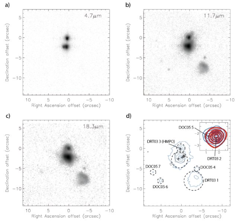
Figure 3: Images of the G45.07+0.13 field taken at a) 4.7 $\mu$m, b) 11.7 $\mu$m, and c) 18.3 $\mu$m at Gemini South with T-ReCS. d) A contour plot (smoothed by 0$\farcs$27) of the 11.7 $\mu$m image (blue contours) of the field showing sources with their labels and encircled with dashed lines that represent the apertures used for photometry. These aperture radii are given in the notes in Table 4. In the upper-right corner there is a blow-up of the the region encompassed by the square. This blow-up shows contours of the double source, DRT03 2 and DOC05 5, at 4.7 $\mu$m and is overlaid (red contours) with the 2 cm radio continuum contours from Hofner & Churchwell (1996). Also plotted as crosses are the locations of the water maser groups as given by Hofner & Churchwell (1996). The origin of each panel is the mid-infrared peak of the HMPO candidate (R.A.(J2000) = 19^h 13^m $22\hbox to0.0pt{.\hss}^{s}07$, Decl.(J2000) = $+10^{\circ}$ $50^{\prime}$ $55\farcs 4$).

The observations of De Buizer et al. (2003) showed that there are three mid-infrared sources at this location, all within 8$\arcsec$ of each other. The brightest mid-infrared source on the field is coincident with the UC H II region. However, at a location $\sim$2$\arcsec$ north of the UC H II region there is a group of water masers associated with a mid-infrared source that has no cm radio continuum emission (Figure 3). De Buizer et al. (2003) showed that this northern mid-infrared source, DRT03 3, has a very bright mid-infrared luminosity of $\sim$4$\times$10³ L_⊙. Assuming that the mid-infrared luminosity is equal to the bolometric luminosity (a gross underestimate), DRT03 3 has the equivalent luminosity of a B0 star. We therefore have a source luminous enough to be a massive protostar, situated at the location of a group of water masers, yet this source has no cm radio continuum emission of its own. For these reasons, De Buizer et al. (2003) claim that DRT03 3 is the true HMPO in this field.

Although there are multiple sources of thermal dust emission present here, it does appear from the high spatial resolution CS maps of Hunter, Phillips, and Menten (1997) that the stellar source powering the UC H II region is the only viable source of the outflow in the region (contrary to what was stated by De Buizer et al. 2003). Since no such tracers are seen coming from the HMPO candidate, this perhaps confirms the youth of the object, placing it in a stage of formation before the onset of an outflow. While the resolution of the 800 and 450 $\mu$m maps of Hunter, Phillips, & Menten (1997) are too coarse to ascertain which mid-infrared source may be dominating the emission at these longer wavelengths, their higher resolution ($\sim$2$\arcsec$) 3 mm map shows no emission from the location of DRT03 3, though emission is detected towards the other two mid-infrared sources on the field.

Our new observations of this field with Gemini have revealed the presence of four more faint mid-infrared sources present (Figure 3) in addition to those already found by De Buizer et al. (2003). It appears that this may be a small cluster of star formation centered on the O9 star powering the UC H II region. DRT03 3 is seen at all 11 mid-infrared wavelengths, as is the UC H II region (DRT03 2). Table 4 lists the flux densities for all mid-infrared sources on the field. Unfortunately, we have no detections of the HMPO candidate alone at any wavelength on the Rayleigh-Jeans side of the SED, and have to rely upon integrated flux density measurements from the whole region (Su et al. 2004) as upper limits to constrain the models.

4 Modeling

4.1 Description of the Model

We will calculate the SED of a HMPO by modeling it as an envelope of gas and dust that is freely falling onto a recently formed massive central star, which is responsible for the heating. Osorio, Lizano & D’Alessio (1999) modeled the SED of a sample of such objects by assuming that the envelope has spherical symmetry. For that work, only upper limits were available for the mid-infrared flux densities of most of the sources. Because this wavelength range is very sensitive to the geometry of the source, here we extend that work by including rotation and flattening of the envelope in the models, so that the results can be tested with the new mid-infrared data presented in this paper. For this purpose, we have followed procedures similar to those already developed in low-mass star models (Osorio et al. 2003).

Envelopes with a density distribution such as that given by Terebey, Shu, & Cassen (1984, hereafter TSC envelopes) assume that the rotation of the infalling material becomes important only in the vicinity of the centrifugal radius, $R_{c}=r_{0}^{4}\Omega_{0}^{2}/GM_{*}$, where $\Omega_{0}$ is the angular velocity (assumed to be constant and small) at a distant reference radius $r_{0}$, and $M_{*}$ is the mass of the central protostar.

The TSC envelopes are flattened only in the inner region, being essentially spherical in the outer region. The inner regions ($r<r_{0}$) of these envelopes are described by the solution of Cassen & Moosman (1981) and Ulrich (1976) (hereafter referred as CMU). The solution is determined by specifying the velocities and densities at the (distant) reference radius $r_{0}$, where the velocity is nearly equal to the radial free-fall value, with only a small azimuthal component corresponding to a constant angular velocity, and the density is set by the required mass infall rate $\dot{M}$. With these assumptions, the density of the inner envelope ($r<r_{0}$) is given by

$$\rho_{\rm CMU}(r,\theta)={{\dot{M}}\over{4\pi(GM_{*}r^{3})^{1/2}}}$$

$$\times{\left(1+{\cos\theta\over\cos\theta_{o}}\right)^{-1/2}}{\left({\cos\theta\over\cos\theta_{0}}+{2R_{c}\cos^{2}\theta_{0}\over r}\right)^{-1}},$$

where $\theta$ and $\theta_{0}$ are the position angles with respect to the rotational symmetry axis of the system at radial distances from the central mass $r$ and $r_{0}$, respectively. At large distances ($r\gg R_{c}$) the motions are radial ($\theta\rightarrow\theta_{0}$) and the density tends to the density distribution for radial free-fall at constant mass infall rate. For $r\lesssim R_{c}$, the motions become significantly non-radial, and the angular momentum of the infalling material causes it to land on a disk ($\theta=90^{\circ}$) at distances $0\leq r\leq R_{c}$. Therefore, $R_{c}$ is the largest radius on the equatorial plane that receives the infalling material.

A more complex description can be given in terms of intrinsically flattened envelopes, such as those with the density distribution resulting from the gravitational collapse of a sheet initially in hydrostatic equilibrium (Hartmann et al. 1994; Hartmann, Calvet, & Boss 1996). These envelopes are flattened not only in their inner region, because of rotation (as the TSC envelopes), but also at large scales due to the natural elongation of the cloud. If the rotational axis is perpendicular to the plane of the self-gravitating layer, the density distribution of the infalling material will be axisymmetric and can be written as:

$$\rho(r,\theta)=\rho_{\rm CMU}(r,\theta)\eta\cosh^{-2}(\eta\cos\theta_{0})\tanh^{-1}(\eta),$$

where $\rho_{\rm CMU}$ is the CMU density distribution for the same $\dot{M}$ and $R_{c}$, and $\eta$ is a measure of the degree of flattening (Hartmann et al. 1996). The degree of flattening in these envelopes is measured by the parameter $\eta\equiv R_{\rm out}/H$, where $R_{\rm out}$ is the outer radius of the envelope and $H$ is the scale height. Hereafter, we will designate them as $\eta$-envelopes.

The scale of this density distribution can be set by using the parameter $\rho_{1}$, defined as

$$\rho_{1}\equiv{{\dot{M}}\over{4\pi(2GM_{*}r_{1}^{3})^{1/2}}},$$

where $r_{1}$ is a reference radius. This reference density corresponds to the density that a spherically symmetric free-falling envelope with the same mass accretion rate, $\dot{M}$, would have at the reference radius $r_{1}$. In our modeling, we will use $r_{1}=1$ AU, and we will designate the reference density as $\rho_{\rm 1\,AU}$.

The remaining parameters that define the density distribution of the $\eta$-envelopes are the centrifugal radius, $R_{c}$, and the inclination of the polar (rotational) axis to the line of sight, $i$. Since $\eta$-envelopes are flattened not only in their inner region but also at large scales most of their material is accumulated over the equatorial plane, having an extinction lower than a TSC envelope of the same mass provided the line of sight is not oriented too close to the edge-on position. Therefore, a flattened $\eta$-envelope model predicts stronger near and mid-infrared emission and less deep absorption features than those predicted by a TSC envelope model of the same mass. Given that our sources are strong mid-infrared emitters, we will preferentially use the $\eta$-envelope density distribution to model our sources.

The temperature distribution along the envelope, as well as the SED from 2 $\mu$m to 2 cm, are determined following the procedures described by Kenyon, Calvet, & Hartmann (1993, hereafter KCH93), Calvet et al. (1994), Hartmann et al. (1996), and Osorio et al. (2003). For a given luminosity of the central star, $L_{*}$, which is assumed to be the only heating source (i.e., neglecting other possible sources of heating such as accretion energy from a disk or the envelope), the temperature structure in the envelope is calculated from the condition of radiative equilibrium, using the approximation of an angle-averaged density distribution. Nevertheless, the emergent flux density is calculated using the exact density distribution. Because we want to compare our results with high spectral resolution mid-infrared data, our model spectra wavelengths were finely sampled ($\Delta$log$\lambda$ = 0.02) in the range 3-25 $\mu$m in order to define with high spectral resolution the 10 $\mu$m silicate absorption feature. Outside this range, wavelengths were sampled at $\Delta$log$\lambda$ = 0.2-0.3. Additionally, in order to make a proper comparison with the observations, we convolved our results with the T-ReCS filter transmission profile. Given that the spectral response of the filters is fairly constant, we do not find large variations (only $\sim$5%) between the averaged and original spectrum.

In our models we use a recently improved dust opacity law, corresponding to a mixture of compounds that was adjusted by matching the observations of the well known low-mass protostar L1551 IRS5 (Osorio et al. 2003). This mixture includes graphite, astronomical silicates, troilite and water ice, with the standard grain-size distribution of the interstellar medium, $n(a)\propto a^{-3.5}$, with a minimum size of 0.005 $\mu$m and a maximum size of 0.3 $\mu$m. The details of the dust opacity calculations are described by D’Alessio, Calvet, & Hartmann (2001).

The inner radius of the envelope, $R_{\rm in}$, is taken to be the dust destruction radius, that is assumed to occur at a temperature of 1200 K, corresponding to the sublimation temperature of silicates at low densities (D’Alessio 1996). The centrifugal radius is assumed to be considerably larger than the dust destruction radius in order to have a significant degree of flattening due to rotation in the inner envelope. The outer radius of the envelope, $R_{\rm out}$, is obtained from our 11.7 $\mu$m images.

In summary, once the dust opacity law and the inner and outer radius of the envelope are defined, the free parameters of our model are $\eta$, $\rho_{\rm 1\,AU}$, $R_{c}$, $i$, and $L_{*}$. In the following, we will discuss on the contribution of these parameters to the resulting SED.

4.2 Behavior of the SED

In order to illustrate the effect of the flattening of the envelope, we have calculated the resulting SED for a TSC envelope and compared it with an $\eta=2$ envelope of the same mass. The results are shown in Figure 4, where it can be seen that the flattened $\eta=2$ envelope predicts stronger near and mid-infrared emission, and less deep absorption features than the TSC envelope, both for low ($i=30^{\circ}$) and moderately high ($i=60^{\circ}$) inclination angles. This behavior is a consequence of the flatter distribution of material in the $\eta=2$ envelope, resulting in an extinction lower than the TSC envelope over a wide range of viewing angles (except for a nearly edge-on view, $i=90^{\circ}$, where the behavior would be the opposite). Thus, in general, the flattened $\eta$-envelopes allow the escape of a larger amount of near and mid-infrared radiation, and consequently they predict stronger flux densities than the TSC envelopes in this wavelength range. Since our sources are strong infrared emitters, in our models we will use $\eta$-envelopes with a significant degree of flattening, $\eta$, of the order of 2.

The observed SEDs of our sources are well sampled in the near and mid-infrared wavelength range. However, this wavelength coverage in insufficient for the models to determine the value of the bolometric luminosity (that we take to coincide with the stellar luminosity, $L_{*}$). The bolometric luminosity is well constrained by the far-infrared data (where the peak of the SED occurs), and to a less extent by the submillimeter or millimeter data. Unfortunately, the available far-infrared data for our sources do not have the appropriate angular resolution to avoid contamination from other nearby sources, and should be considered as upper limits, while millimeter data are only available for one of our sources. Therefore, in general, we constrain the value of the luminosity by fitting the mid-infrared data closer to the SED peak, that are helpful to set a lower limit for the luminosity.

On the other hand, the depth and shape of the silicate absorption feature (which is very well delineated by our mid-infrared data) determines the extinction along the line-of-sight, that in turn is related to the inclination angle, $i$, the density scale, $\rho_{1}$, and the centrifugal radius, $R_{c}$. The depth of the 10 $\mu$m silicate absorption increases not only with the density scale of the envelope, but also with the inclination angle, since the extinction is much smaller along the rotational pole ($i=0$) than along the equator ($i=90^{\circ}$) (see Osorio et al. 2003). Thus, the behavior of the parameters $\rho_{1}$ and $i$ is somewhat interchangeable in the mid-infrared (although such behavior is different at millimeter wavelengths). For instance, an envelope with a combination of low density and high inclination could have an extinction and mid-infrared emission similar to an envelope with a higher density but viewed pole-on. Therefore, for the sources where millimeter data are not available, it is difficult to constrain $i$ and $\rho_{1}$ simultaneously, and we will search for fits both for high as well as for low inclination angles.

The behavior of the SED with the centrifugal radius, $R_{c}$, is more complex. Increasing the value of $R_{c}$ will widen the region of evacuated material, producing an overall decrease of the extinction along the line of sight, but, at the same time, it will result in a decrease of the temperature of the envelope, because the material tends to pile up at larger distances from the source of luminosity. Thus, depending on the wavelength range, one of the two effects will be the dominant. At short wavelengths, where the dust opacity is higher, it is expected that the lower extinction of the envelopes with large values of $R_{c}$ will result in an increase of the observed emission. At longer wavelengths, where the opacity is low enough (except in the silicate absorption feature), the dominant effect is expected to be due to the decrease in the temperature, resulting in a decrease of the observed emission for larger values of $R_{c}$. This is illustrated in Figure 4, where it is shown that the emission of the envelope with $R_{c}=600$ AU dominates in the near-infrared range, while the emission of the $R_{c}=250$ AU envelope dominates at longer wavelengths. As shown in the figure, this result is valid both for low and relatively high inclination angles, although we note that the point where the small $R_{c}$ envelope becomes dominant shifts slightly to longer wavelengths when increasing the inclination angle (from $\sim 2~{}\mu$m for $i=30^{\circ}$ to $\sim 5~{}\mu$m for $i=60^{\circ}$). This shift occurs because envelopes seen at higher inclination angles are more opaque, thus requiring a longer wavelength (where the opacity is lower) for the small $R_{c}$ envelope to become dominant.

Since we expect the value of $R_{c}$ to be of the order of the radius of a possible circumstellar disk, in our modeling we will explore a range of values for $R_{c}$ from tens to hundreds of AUs, depending on the luminosity of the source. The upper limit of this range is suggested by the highest angular resolution observations of disks reported towards massive protostars (e.g., Shepherd, Claussen, & Kurtz 2001), while the lower limit is set by the smallest values recently reported for protoplanetary disks around low-mass YSOs (Rodríguez et al. 2005).

From the values of the parameters obtained from our fits to the observed SEDs we can derive other physical parameters, such as the total mass of the envelope, $M_{\rm env}$, obtained by integration of the density distribution, and the mass of the central star, $M_{*}$, derived from its luminosity, $L_{*}$. Once the mass of the star is known, the mass accretion rate in the envelope, $\dot{M}$, can be derived from the value of $\rho_{1}$.

Yorke (1984) and Walmsley (1995) proposed that some objects could be accreting material at a rate high enough to quench the development of an incipient HII region. These objects would lack detectable free-free emission, being good candidates to be the precursors of the UCHII regions. In the case of spherical accretion, it is easy to show that the critical mass accretion rate required to reduce the HII region to a small volume close to the stellar surface is $\dot{M}_{\rm crit}=(8\pi Gm^{2}_{\rm H}\alpha^{-1}\dot{N}_{i}M_{*})^{1/2}$, where $m_{\rm H}$ is the hydrogen mass, and $\alpha$ is the recombination coefficient (excluding captures to the $n=1$ level). We will adopt the value, $M_{\rm crit}$, as a critical measure of the mass accretion rate required to “choke off” the possible development of an UC H II region. Since we are assuming departures from spherical symmetry in our envelopes, in reality a more complex calculation would be required to accurately derive the corresponding critical mass rate. However, for simplicity we will assume that if the ratio between the mass accretion rate in our envelope and the critical spherical mass accretion rate $\dot{M}/\dot{M}_{\rm crit}\gg 1$, it would indicate that photoionized emission is not expected to be detectable in the source.

5 Comparison of the Models with the Observations

In this section, we estimate the physical parameters of the three HMPO candidates by fitting our models to the observed SEDs, using also the available information on size and morphology inferred from the images. Given that spherical envelopes do not appear to be able to account for the observed properties of the SEDs in the mid-infrared, we have modeled the sources using $\eta$-envelopes with a significant degree of elongation (see discussion in $\S$4.2). Since the temperature distribution in the envelopes is estimated using the approximation of an angle-averaged density distribution, valid for moderately elongated envelopes, we did not attempt to consider very high values of $\eta$, that correspond to extremely elongated envelopes where the temperature calculations probably would not be accurate enough. Therefore, we explored values of $\eta$ around 2, and in all three sources we were able to get good fits for $\eta=2.5$. We note that this value coincides with the one that provided the best fit for the low-mass protostar L1551-IRS5, after exploring a wide range of values of the $\eta$ parameter (Osorio et al. 2003).

Given the incomplete and non-uniform coverage of the observed SED, the fitting process cannot be automated and should be carried out manually on a case-by-case basis. As was already mentioned in the previous section, the luminosity is well constrained by the peak of the SED, that is expected to happen in the far-infrared. Unfortunately, at present, far-infrared observations do not reach the angular resolution required to properly isolate the emission of these distant sources from contamination of other sources in their vicinity. Therefore, in general, the far-infrared data are considered only as upper limits and we have to use the mid-infrared data to obtain a range of possible values for the luminosity. Thus, the general strategy was to first run a set of models with increasing luminosities until we found a value that was able to reproduce the observed mid-infrared flux density near the peak of the SED and consistent with the millimeter and submillimeter data. Once an approximate value of the luminosity was found, we proceeded to run a set of models to find the density scale, which is then basically determined by the millimeter and submillimeter data points. When the density scale was fixed, we ran models with different inclinations in order to find the best fit to the absorption feature in the mid-infrared, which is particularly sensitive to the value of the inclination angle. Finally, we refined the modeling by testing a range of possible values of the centrifugal radius.

If the data point coverage of the SED is good enough we should end this process with essentially one final model (the “best fit model”) that is able to reproduce the observed data points within the constrains imposed by the observational uncertainties. In the case that only upper limits are available in the millimeter and submillimeter domain, the density scale and inclination angle cannot be constrained simultaneously, and in this case we present two fits, one for a low inclination angle, and a second one for a high inclination angle. The value of the centrifugal radius not well constrained in this case either. However, on the basis of an additional analysis of the quality of the data points and the peculiarities of each source (see discussion of individual sources) we attempt to favor one of the fits as the best fit model.

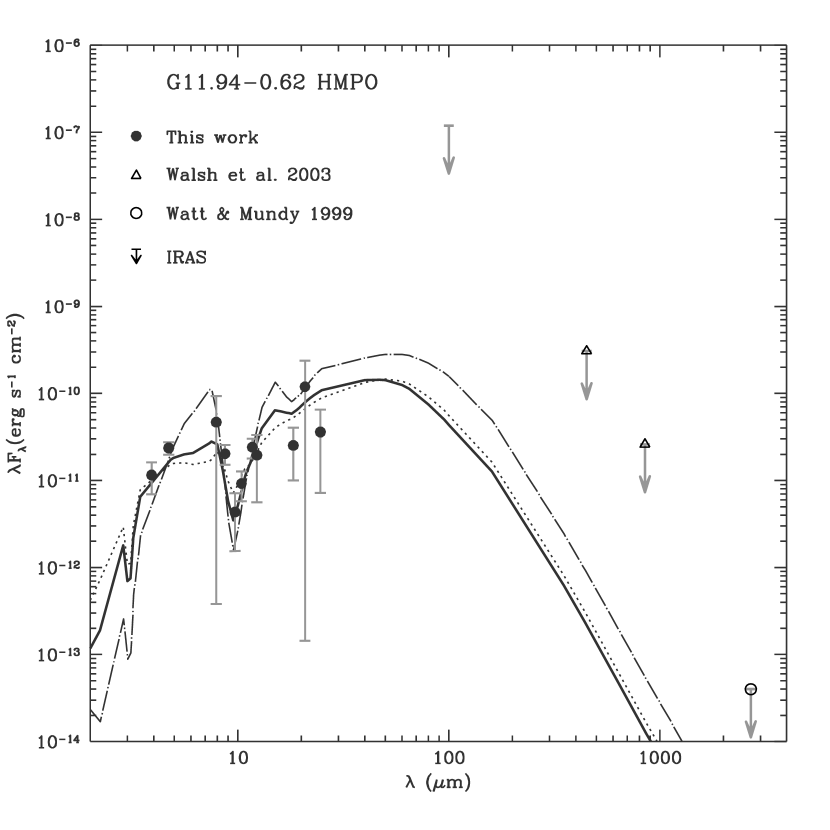
Figure 5: Observed and model SEDs for the source G11.94-0.62 HMPO. The different symbols represent the observed values of the flux density. Error bars are 3-$\sigma$. Upper limits are represented by arrows. Solid-line represents the best fit model, obtained with $i=53^{\circ}$, $R_{c}=30$ AU, $L_{*}=75~{}L_{\odot}$, $\rho_{\rm 1\,AU}=2\times 10^{-13}$ g cm^-3 (see Table 5), while the dotted line represents a model with the same $i$ and $\rho_{\rm 1\,AU}$ but with $R_{c}=100$ AU. Dot-dashed line represents a model with a low inclination angle of $i=30^{\circ}$, with $R_{c}=30$ AU and $\rho_{\rm 1\,AU}=7.5\times 10^{-13}$ g cm^-3. The adopted distance is 4.2 kpc (Hofner & Churchwell 1996).

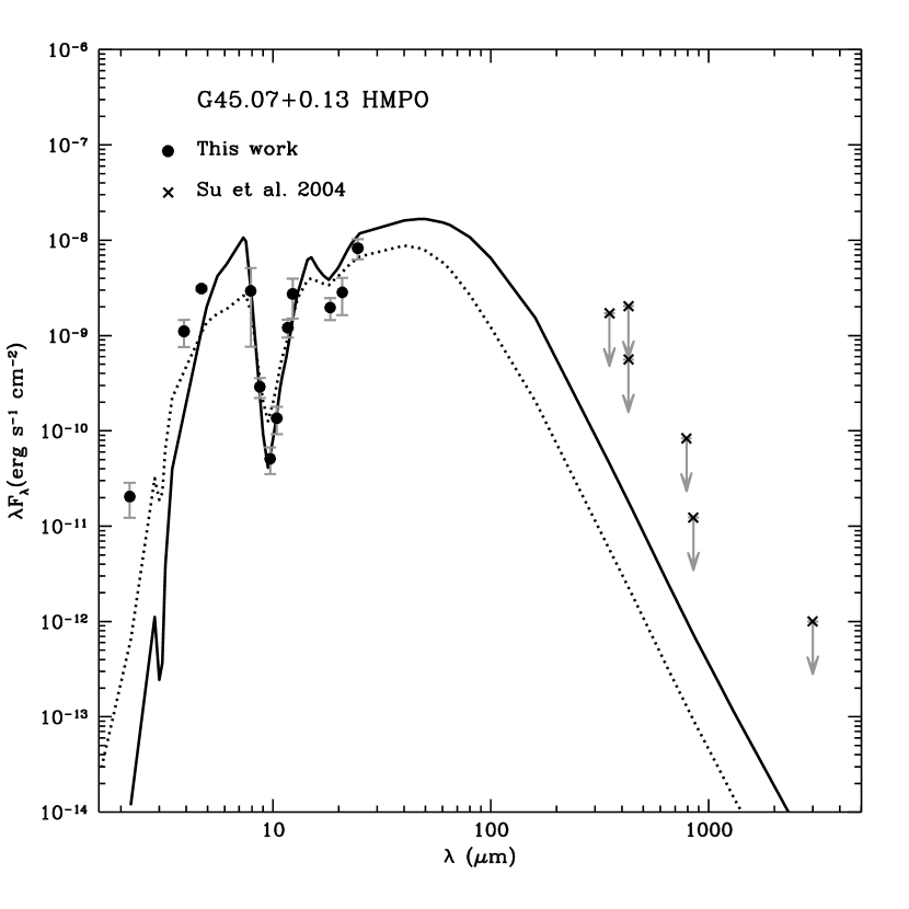
Figure 7: Observed and model SEDs for the source G45.07+0.13 HMPO. The different symbols represent the observed values of the flux density. Error bars are 3-$\sigma$. Upper limits are represented by arrows. Solid line represents the best fit model, obtained with $i=30^{\circ}$, $R_{c}=370$ AU, $L_{*}=2.5\times 10^{4}~{}L_{\odot}$, and $\rho_{\rm 1\,AU}=5.3\times 10^{-12}$ g cm^-3 (see Table 5). Dotted line represents a model with the same luminosity and a higher inclination angle, $i=58^{\circ}$, with $R_{c}=270$ AU, and $\rho_{\rm 1\,AU}=7.5\times 10^{-13}$ g cm^-3. The adopted distance is 9.7 kpc (Wood & Churchwell 1989).

Table 5 lists the values of the parameters of our best fit models: the inner, outer and centrifugal radii of the envelope, the stellar luminosity, the reference density at 1 AU, and the inclination angle. Our best-fit model SEDs are shown in Figures 5, 6, and 7. Table 6 lists other derived parameters for each source: the mass of the envelope, its temperature at a radius of 1000 AU, the mass and spectral type of the central protostar, the mass accretion rate, the rate of ionizing photons, and the critical mass accretion rate. These parameters have been derived following the procedures explained in the footnotes to the table.

5.1 G11.94-0.62 HMPO

This HMPO has been observed through continuum measurements at millimeter (Watt & Mundy 1999), submillimeter (Walsh et al. 2003), and mid-infrared wavelengths. The submillimeter data will be used in our modeling only as upper limits, since they have been obtained with a large beam ($10^{\prime\prime}$-$18^{\prime\prime}$) and therefore it is not possible to separate the emission of the nearby UC H II region from that of the HMPO. Likewise, the millimeter flux densities will be used also as upper limits, since the analysis of Watt & Mundy (1999) suggests that the millimeter emission observed towards this source corresponds to free-free emission of the nearby UC H II region with a negligible contribution from dust.

In general, to constrain the physical parameters of the sources, we use the observed SED as well as the information on size and morphology given by the images. However, the G11.94$-$0.62 HMPO source appears unresolved in the near and mid-infrared images (see Figure  1) and therefore, we have only an upper limit for its size.

Because we considered the far-infrared, submillimeter and millimeter data only as upper limits, the luminosity of this source is constrained essentially by the data at wavelengths near 20 $\mu$m, that indicate that this is a low luminosity source. We obtain a value of 75 $L_{\odot}$ for the luminosity of this object, corresponding to a A0 star of 5 $M_{\odot}$. Since we only have upper limits for the flux densities in the submillimeter-millimeter wavelength range, we cannot constrain the density and inclination simultaneously. Therefore, we searched for fits both at low ($i$=20^∘-30^∘) and high inclination angles ($i$=50^∘-60^∘). At low inclination angles, we obtained a quite good fit for $i=$30^∘, $\rho_{\rm 1\,AU}=7.5\times 10^{-13}$ g cm^-3, and $R_{c}=30$ AU (dot-dashed line in Figure 5), but this model predicts too much emission at 18.3 and 24.6 $\mu$m. In order to reproduce the observational data in the 18-25 $\mu$m wavelength range, we require models with a high inclination angle. Our best fit model is obtained for a high inclination angle, $i=53^{\circ}$, with $\rho_{\rm 1\,AU}=$ 2$\times 10^{-13}$ g cm^-3 ($M_{env}=1~{}M_{\odot}$), and $R_{c}=30$ AU (solid line in Figure 5). We can obtain reasonable fits for $1\times 10^{-13}<\rho_{\rm 1\,AU}<4\times 10^{-13}$ g cm^-3 and $20<R_{c}<200$ AU. For example, a model with $R_{c}=100$ AU is also feasible (dotted line in Figure 5). However, we favor the $R_{c}=30$ AU model (solid line in Figure 5, and Tables 5 and 6) because it reproduces better the flux densities shortward of 8.7 $\mu$m and the depth of the 10 $\mu$m silicate absorption feature.

For our favored model, the ratio $\dot{M}/\dot{M}_{\rm crit}\gg 1$ (see Table 6). Therefore, the source could not develop a detectable H II region. Furthermore, since the luminosity obtained in this model is quite low, free-free emission from the HMPO would be hardly detectable, even in the case of a negligible accretion rate. Thus, G11.94-0.62 is not luminous enough to be considered as a HMPO. Most likely, given the low temperature of the envelope ($T_{\rm 1000\,AU}=40$ K), it would be better considered as a “warm core” that is forming an intermediate-mass star, with an infall rate more than one order of magnitude higher than the typical infall rates of low-mass protostars (see KCH93).

5.2 G29.96-0.02 HMPO

The G29.96-0.02 HMPO is the only source of our sample that appears to be associated with strong millimeter emission. Thus, for this source we have both infrared and millimeter data to constrain better the models. The strong millimeter emission suggests a dense or luminous envelope. In addition, the relatively strong near-infrared emission observed suggests that the envelope should be seen nearly pole-on, since in this direction there is a decrease of the density with respect to the equatorial plane that allows the escape of near-infrared radiation.

A reasonable fit (solid-line in Figure 6), explaining simultaneously the strong millimeter emission as well as the near-infrared flux densities, is obtained by assuming an extremely dense ($\rho_{\rm 1\,AU}=3.1\times 10^{-11}$ g cm^-3), and therefore very massive envelope ($M_{env}=576~{}M_{\odot}$), with a centrifugal radius of $R_{c}=570$ AU, seen with a low inclination angle ($i=12^{\circ}$), and heated by a luminous ($L_{*}=1.8\times 10^{4}~{}L_{\odot}$) B1 star (see Tables 5 and 6). This value of the luminosity is a lower limit, since it is the smallest value that is consistent with the mid-infrared and millimeter data points, and we estimate that it can be higher up to a factor of three. Likewise, we estimate that the uncertainty in the density scale is $\sim$30%, and that the range of plausible values is $10^{\circ}<i<20^{\circ}$ for the inclination angle, and $500<R_{c}<1200$ AU for the centrifugal radius. Note that the 9.7 $\mu$m data point is only an upper limit, and therefore it does not set the depth of the silicate absorption feature. Also, we want to point out that we have not attempted that our models reproduce the exact values of the observational data points in the millimeter range, due to the problems discussed in §3.2 and because errors are not available for some of these data points.

Our best fit model predicts that the flux density at 3.9 $\mu$m should be lower than the value observed. We think that the excess of flux density observed at wavelengths shorter than 3.9 $\mu$m could be due to scattered light in a cavity carved out by the outflow associated with G29.96$-$0.02 HMPO (Gibb et al. 2004). In fact, Gibb et al. (2004) suggest that scattered light in G29.96$-$0.02 HMPO could be dominant even at 18 $\mu$m. However, our models show that the emission from 4-18 $\mu$m can be reproduced as dust emission from an infalling flattened envelope, and that scattered light may only be dominant for wavelengths shorter than $\sim$4 $\mu$m.

From Table 6 we see that the ratio ${\dot{M}}/{\dot{M}_{crit}}=22,000$. Thus, we do not expect the development of an H II region in the G29 HMPO. This is consistent with the lack of strong free-free emission at the position of the source.

In order to illustrate the relevance of the millimeter constraints, in Figure 6 we show an additional model (dotted-line), obtained by fitting only the mid-infrared observations. For this model, we obtain a value of the luminosity of only 2400 $L_{\odot}$, a density scale of $5.3\times 10^{-12}$ g cm^-3 and an envelope mass of $\sim$ 98 $M_{\odot}$. This set of parameters fits very well the mid-infrared data; however the model predicts far too little emission at long wavelengths, underestimating by almost one order of magnitude the luminosity and mass. These results illustrate that both millimeter as well as mid-infrared data are required in order to determine reliable values of the derived parameters.

It is worthwhile to mention that our models can fit the observed SED with a value of $R_{c}\simeq 570$ AU, considerably smaller than the size of the elongated structures observed towards the G29.96-0.02 HMPO ($\gtrsim$ 10,000 AU, Olmi et al. 2003) and some other high-mass protostars (1000-30000 AU, see Cesaroni 2005 and references therein). These structures have been interpreted by some authors as tracing large-scale disks or rotating toroids. Our results suggest that these structures could be naturally explained as infalling flattened envelopes (with sizes of thousands of AUs), rather than as large circumstellar disks. The formation of such disks is expected to occur at a scale of the order of $R_{c}$, which according to our models could be of the order of hundreds of AUs.

5.3 G45.07+0.13 HMPO

In order to compare the predicted SED of the G45.07+0.13 HMPO with the data, we use the existing millimeter observations (taken from Su et al. 2004) only as upper limits, since they do not have an angular resolution high enough to separate the HMPO emission from that of the UC H II region. Therefore, we will restrict our comparison to our mid-infrared observations.

The G45.07+0.13 HMPO exhibits an anomalous spectrum because in spite of its deep silicate absorption (indicative of a large extinction), it presents a very strong emission in the near-infrared range (4-8 $\mu$m). For this source, we also have considered models for both high and low inclination angles. A model with a highly inclined envelope ($i=58^{\circ}$), a density scale of $\rho_{\rm 1\,AU}=7.5\times 10^{-13}$ g cm^-3, and a centrifugal radius of $R_{c}=$270 AU (dotted line in Figure 7) predicts too little emission at 4.7 $\mu$m and shorter wavelengths, and also presents a silicate absorption feature that is too weak. Alternatively, an envelope with a lower inclination ($i=35^{\circ}$), a larger density scale ($\rho_{\rm 1\,AU}=5.3\times 10^{-12}$ g cm^-3), and a centrifugal radius of $R_{c}=$370 AU (solid line in Figure 7 and Table 5) reproduces better the emission at 4.7 $\mu$m as well as the depth of the silicate absorption, although it still has problems in explaining the emission at the shortest wavelengths ($\sim 2~{}\mu$m). Both models require the same luminosity ($L_{*}=2.5\times 10^{4}$ $L_{\odot}$), implying a B1 star of 13 $M_{\odot}$.

We favor the low inclination model (solid line in Figure 7 and Tables 5 and 6) because it can explain reasonably well most of values of the observed flux density. As we discussed for the G29.96-0.02 HMPO case, the excess of flux density observed at wavelengths shorter than 3.9 $\mu$m could be due to scattered light. By running other models with slightly different values of the parameters, and taking into account the upper limits set by the submillimeter and millimeter data, we estimate uncertainties of $\pm 5^{\circ}$ in the inclination angle, a factor of two in the density scale and the centrifugal radius, and a factor of three in the luminosity with respect to the values given in Table 5.

For the values given in Table 6, a ratio $\dot{M}/\dot{M}_{\rm crit}=3600$ is derived. Thus, as in the previous sources, the mass accretion rate for the G45.07+0.13 HMPO is high enough to quench the development of an UC H II region, that is consistent with the lack of detected free-free emission towards this HMPO.

6 Summary

We have obtained mid-infrared data for four HMPO candidates at Gemini Observatory. These data have the subarcsecond angular resolution necessary to isolate the emission of the HMPO candidates from that of nearby sources. The data are well-sampled across the entire 2 to 25 $\micron$ atmospheric windows, and particularly throughout the 10 $\micron$ absorption feature.

Since this wavelength range is very sensitive to the source geometry, we have constructed a grid of SED models for the physical conditions (density, temperature, luminosity) expected for the early stages of massive star formation, and taking into account for the first time the rotation as well as the natural flattening of the infalling envelopes. These models reach a degree of complexity comparable to those developed for low-mass protostars. Using our mid-infrared data, as well as the far-infrared and millimeter constraints available in the literature, we have fit the SEDs of the HMPO candidates in G11.94$-$0.62, G29.96$-$0.02, and G45.07+0.13, inferring physical parameters for the infalling envelopes as well as for the central stars.

Our main conclusions are the following:

1. The HMPO candidate in G11.94-0.62 does not seem to be luminous enough to be considered as a HMPO. Most likely, it would be better considered as a “warm” core that is forming an intermediate-mass star, with an infall rate more than one order of magnitude higher than the typical infall rates of low-mass protostars.

2. The candidates G29.96$-$0.02 and G45.07+0.13 appear to be genuine HMPOs with high luminosities, $L_{*}\simeq 20000~{}L_{\odot}$, and high accretion rates, $\dot{M}\simeq 10^{-3}$-$10^{-2}~{}M_{\odot}$ yr^-1. These values of the mass accretion rate exceed by several orders of magnitude the critical value required to quench the development of an UC H II region. Therefore, these sources appear to be in a very early stage, previous to the development of an UC H II region.

3. Our models are able to fit the observed SEDs of the HMPOs with values of the centrifugal radius of a few hundred AUs, which are considerably smaller than the size of the elongated structures observed towards some high-mass protostars (1000-30000 AU). These structures have been interpreted by some authors as tracing large-scale disks or rotating toroids. Our results suggest that these structures could be naturally explained as infalling flattened envelopes (with sizes of thousands of AUs), rather than as large circumstellar disks. The formation of such disks is expected to occur at a scale of the order of $R_{c}$, which according to our models could be of the order of hundreds of AUs.

4. Our detailed modeling suggests that massive star formation can proceed in a way very similar to the formation of low-mass stars. Unfortunately, massive protostars are more distant than low-mass protostars, and the instrumentation currently available in the far-infrared and millimeter ranges does not reach the angular resolution necessary to separate the HMPO emission from that of other nearby sources. Since these wavelength ranges are very important to constrain properly the physical parameters of the sources, such as the luminosity, in general our fit models are not unique. New data in these wavelength domains would be most valuable to determine the physical conditions in the early stages of massive star formation.

Table 1: T-ReCS Filter Information and Integration and Calibration Parameters

Filter		G11.94-0.62			G29.96-0.02			G45.07+0.13
$\lambda_{c}$	$\Delta\lambda$	t	Standard	Fν	t	Standard	Fν	t	Standard	Fν
2.2	2.0-2.4	304	HD169916	447	521	HD196171	283	130	HD187642	550
3.9	3.6-4.1	304	HD178345	67.0	521	HD196171	122	130	HD187642	200
4.7	4.4-5.0	217	HD178345	40.3	521	HD196171	73.5	130	HD187642	137
7.7	7.4-8.1	217	HD178345	17.8	304	HD175775	29.6	130	HD169916	47.7
8.7	8.4-9.1	217	HD169916	38.1	521	HD169916	38.1	130	HD169916	38.1
9.7	9.2-10.2	217	HD169916	32.3	304	HD175775	20.1	130	HD169916	32.3
10.4	9.9-10.9	217	HD169916	28.5	304	HD175775	17.7	130	HD169916	28.5
11.7	11.1-12.2	217	HD169916	22.4	304	HD169916	22.4	130	HD169916	22.4
12.3	11.7-12.9	217	HD169916	20.0	130	HD169916	20.0	130	HD169916	20.0
18.3	17.6-19.1	217	HD178345	3.5		a		130	HD169916	9.6
24.6	23.6-25.5	304	Alpha Cen	27.6		$\cdots$		130	HD187642	5.5

Note: The value ‘$\lambda_{c}$’ is the effective central wavelength of the filter in $\mu$m, and ‘$\Delta\lambda$’ is the wavelength range of the filter using the 50% transmission cut-on and cut-off of the bandpass. The value ‘t’ is the on-source integration time in seconds in the given filter of the given science field. ‘Standard’ is the name of the standard star used in the given filter for the given science field. ‘F_ν’ is the assumed flux density in Jy of the standard star in the given filter.
^a OSCIR data. See De Buizer et al. (2002).

Table 2: Observed flux densities in mJy for sources on G11.94-0.62 field

$\lambda$a	DRT03 1 (HMPO)b	DRT03 2c,d	DRT03 3c,e	DRT03 4c,f	DRT03 5c,g	DRT03 6h
$3.9{\micron}$	15$\pm$2	40$\pm$5	71$\pm$8	34$\pm$4	29$\pm$3	52$\pm$7
$4.7{\micron}$	37$\pm$2	87$\pm$6	134$\pm$8	106$\pm$5	85$\pm$3	107$\pm$9
$7.7{\micron}$	123$\pm$44	858$\pm$308	2250$\pm$808	1240$\pm$446	854$\pm$308	2420$\pm$871
$8.7{\micron}$	59$\pm$5	505$\pm$43	669$\pm$57	523$\pm$45	433$\pm$37	564$\pm$48
$9.7{\micron}$	14$\pm$3	170$\pm$20	118$\pm$17	120$\pm$15	99$\pm$11	113$\pm$18
$10.4{\micron}$	32$\pm$4	412$\pm$51	240$\pm$30	335$\pm$42	296$\pm$37	277$\pm$35
$11.7{\micron}$	94$\pm$8	1210$\pm$104	1010$\pm$87	1150$\pm$99	988$\pm$85	816$\pm$71
$12.3{\micron}$	80$\pm$19	1350$\pm$316	1340$\pm$316	1300$\pm$305	1050$\pm$247	1100$\pm$258
$18.3{\micron}$	154$\pm$31	11300$\pm$2000	8800$\pm$1570	11600$\pm$2070	7000$\pm$1250	8230$\pm$1470
$20.8{\micron}$i	829$\pm$340	5430$\pm$800	7820$\pm$1200	11300$\pm$1640	11100$\pm$1530	$\cdots$ j
$24.6{\micron}$	296$\pm$79	35800$\pm$3200	33600$\pm$3040	53500$\pm$4800	28700$\pm$2590	$\cdots$ j

Note: Errors given to the flux values are 1-$\sigma$ errors that are quadrature addition of the photometric and calibration errors.
^a Effective central filter wavelength.
^b Integrated flux density in a 0$\farcs$6 radius aperture centered on the HMPO candidate.
^c This is an extended emission source and is not fully resolved from other sources on the field.
^d Integrated flux density in a 2$\farcs$1 radius aperture centered on the center of the extended mid-infrared emission from this source.
^e Integrated flux density in a 2$\farcs$7 radius aperture centered on the center of the extended mid-infrared emission from this source.
^f Integrated flux density in a 1$\farcs$8 radius aperture centered on the center of the extended mid-infrared emission from this source.
^g Integrated flux density in a 1$\farcs$2 radius aperture centered on the center of the extended mid-infrared emission from this source.
^h This single extended source was labeled as two individual sources in the work of De Buizer et al. (2003, 2005), however the observations presented here show it to be a very large and amorphous single but extended source. The integrated flux density is from a 3$\farcs$1 radius aperture centered on the center of the extended mid-infrared emission from this source.
ⁱ From MIRLIN/IRTF data used in De Buizer et al. (2003, 2005).
^j Source partially off field at this wavelength so no flux density given.

Table 3: Observed flux densities in mJy for sources on G29.96-0.02 field

$\lambda$a	HMPOb	HMPO($+$bg)c	UC HIId
$2.2{\micron}$	$<$5	14 $\pm$2	327$\pm$24
$3.9{\micron}$	38 $\pm$5	112 $\pm$10	4300$\pm$368
$4.7{\micron}$	123 $\pm$12	321 $\pm$6	10800$\pm$183
$7.7{\micron}$	66 $\pm$20	492 $\pm$85	37400$\pm$6440
$8.7{\micron}$	13 $\pm$2	437 $\pm$31	77800$\pm$5550
$9.7{\micron}$	$<$25	239 $\pm$26	56000$\pm$6090
$10.4{\micron}$	13 $\pm$3	370 $\pm$45	80000$\pm$9700
$11.7{\micron}$	197 $\pm$32	1130 $\pm$86	141000$\pm$10800
$12.3{\micron}$	345 $\pm$78	1680 $\pm$342	169000$\pm$34000
$18.3{\micron}^{e}$	2280$\pm$340	16400$\pm$1640	462000$\pm$46000

Note: Values preceded by a ‘$<$’ means it is a 3-$\sigma$ upper limit of the source flux within the apertures specified in the table notes below. Errors given to the flux values are 1-$\sigma$ errors that are quadrature addition of the photometric and calibration errors.
^a Effective central filter wavelength.
^b Integrated flux density after subtraction of background due to extended flux from the UC H II region.
^c Integrated flux density in a 1$\farcs$25 radius aperture centered on the HMPO peak without subtraction of the background UC H II region.
^d Integrated flux density in a 6$\farcs$4 radius aperture centered on the center of the extended mid-infrared emission from the UC H II region.
^e From OSCIR data used in De Buizer et al. (2002).

Table 4: Observed flux densities in mJy for sources on G45.07+0.13 field

$\lambda$a	DRT03 1b	DRT03 2c	DRT03 3 (HMPO)d	DOC05 4e	DOC05 5f	DOC05 6g	DOC05 7g
$2.2{\micron}$	$<$14	17$\pm$2	15$\pm$2	$<$4.04	8$\pm$2	$<$4.04	$<$4.04
$3.9{\micron}$	62 $\pm$7	1460$\pm$156	1440$\pm$153	$<$3.1	567$\pm$60	$<$3.1	$<$3.1
$4.7{\micron}$	153 $\pm$10	4950$\pm$81	4880$\pm$80	$<$8.3	1610$\pm$27	$<$8.3	$<$8.3
$7.7{\micron}$	1330 $\pm$331	13700$\pm$3390	7750$\pm$1910	72$\pm$20	2710$\pm$670	25$\pm$12	71$\pm$20
$8.7{\micron}$	475 $\pm$38	5940$\pm$467	841$\pm$66	24$\pm$3	996$\pm$78	9$\pm$2	14$\pm$2
$9.7{\micron}$	233 $\pm$27	2080$\pm$197	165$\pm$17	$<$14.6	308$\pm$30	$<$14.6	$<$14.6
$10.4{\micron}$	377 $\pm$41	4350$\pm$461	472$\pm$50	17 $\pm$4	692$\pm$73	9$\pm$3	$<$9.4
$11.7{\micron}$	1260 $\pm$88	18100$\pm$1270	4720$\pm$330	66 $\pm$5	2350$\pm$164	26$\pm$3	19$\pm$3
$12.3{\micron}$	2310 $\pm$347	37100$\pm$5560	11200$\pm$1670	109 $\pm$17	6610$\pm$991	48$\pm$10	61$\pm$11
$18.3{\micron}$	10900$\pm$964	72900$\pm$6360	12000$\pm$1050	544 $\pm$66	8600$\pm$753	$<$136	264$\pm$51
$20.8{\micron}^{h}$	15100$\pm$2130	102000${}^{i}\pm$13500	19700$\pm$2780	$\cdots$	$\cdots$	$\cdots$	$\cdots$
$24.6{\micron}$	51700$\pm$4150	564000$\pm$45000	67600$\pm$5400	2170$\pm$208	$\cdots$	335$\pm$119	1338$\pm$159

Note: Values preceded by a ‘$<$’ means it is a 3-$\sigma$ upper limit of the source flux within the apertures specified in the table notes below. Errors given to the flux values are 1-$\sigma$ errors that are quadrature addition of the photometric and calibration errors.
^a Effective central filter wavelength.
^b Integrated flux density in a 2$\farcs$4 radius aperture centered on center of the extended mid-infrared emission from this source.
^c Integrated flux density in a 2$\farcs$0 radius aperture centered on the peak of this source. This source flux density is contaminated by some emission from DOC05 5, which is a close mid-infrared companion. DOC05 5 was fit by a gaussian and subtracted off before the aperture photometry was performed on DRT03 2. However DOC05 5 is much fainter than DRT03 2, so the contamination is relatively small (on order the flux error) at all wavelengths.
^d Integrated flux density in a 1$\farcs$1 radius aperture centered on the peak of this HMPO candidate.
^e Integrated flux density in a 0$\farcs$7 radius aperture centered on the peak of this source.
^f Flux densities quoted for this source are rough estimates. DOC05 5 is faint and separated by only 0$\farcs$7 from the very prominent mid-infrared source DRT03 2. Fluxes for this source were obtained by fitting DRT03 2 by a gaussian and subtracting it away before performing aperture photometry with a 0$\farcs$7 radius aperture. However, as the source was observed at longer and longer wavelengths resolution grew steadily worse until at 24.5$\micron$ the sources could not be resolved.
^g Integrated flux density in a 0$\farcs$7 radius aperture centered on the peak of this source.
^h From MIRLIN/IRTF data used in De Buizer et al. (2003, 2005).
ⁱ This is the combined flux from DRT03 2 and DOC05 5, since they are not resolved from each other using IRTF.

Table 5: Parameters of the Best Fit Models

HMPO	$\eta$	$R_{\rm in}$	$R_{\rm out}$	$R_{\rm c}$	$L_{*}$	$\rho_{\rm 1\,AU}$	$i$
		(AU)	(AU)	(AU)	($L_{\odot}$)	(g cm-3)	(∘)
G11.94-0.62	2.5	2	5000	30	75	1.5$\times 10^{-13}$	53
G29.96-0.02	2.5	245	12000	570	18000	3.0$\times 10^{-11}$	12
G45.07+0.13	2.5	227	9000	370	25000	5.3$\times 10^{-12}$	35

Table 6: Physical Parameters Derived from the Models

HMPO	$M_{\rm env}$	$T_{\rm 1000\,AU}$	$M_{*}$	Spectral	$\dot{M}$	$\dot{N}_{i}$	$\dot{M}_{\rm crit}$
	($M_{\odot}$)	(K)	($M_{\odot}$)	Type	($M_{\odot}$ yr-1)	(s-1)	($M_{\odot}$ yr-1)
G11.94-0.62	1	40	5	A0	$8.7\times 10^{-5}$	$3.0\times 10^{37}$	$3.5\times 10^{-11}$
G29.96-0.02	576	300	11	B1	$2.0\times 10^{-2}$	$1.0\times 10^{46}$	$9.0\times 10^{-7}$
G45.07+0.13	64	200	13	B1	$3.6\times 10^{-3}$	$1.0\times 10^{46}$	$1.0\times 10^{-6}$

Figure 4: (a) Model SEDs for an $\eta=2$ envelope (solid-line) and a TSC envelope (dotted-line) with the same values of the centrifugal radius ($R_{c}=600$ AU) and inclination angle ($i=30^{\circ}$). (b) Same as (a), but for a higher value of the inclination angle ($i=60^{\circ}$). (c) Model SEDs for two $\eta=2$ envelopes, with the same value of the inclination angle ($i=30^{\circ}$) and two different values of the centrifugal radius: $R_{c}=250$ AU (dashed line) and $R_{c}=600$ AU (solid line). (d) Same as (c), but for $i=60^{\circ}$. The stellar luminosity ($L_{*}=25000~{}L_{\odot}$), the mass of the envelope (M${}_{env}=9~{}M_{\odot}$), and the assumed distance (1 kpc) are the same in all models.

References

- Behrend & Maeder (2001) Behrend, R. & Maeder, A. 2001, A&A, 373, 190
- Bronfman et al. (1996) Bronfman, L., Nyman, L.-A., & May, J. 1996, A&AS, 115, 81
- Calvet et al. (1994) Calvet, N., Hartmann, L., Kenyon, S. J., & Whitney, B. A. 1994, ApJ, 434, 330
- Cesaroni et al. (1992) Cesaroni, R., Walmsley, C. M., & Churchwell, E. 1992, A&A, 256, 618
- Cesaroni et al. (1994) Cesaroni, R., Churchwell, E., Hofner, P., Walmsley, C. M., & Kurtz, S. 1994, A&A, 288, 903
- Cesaroni, Hofner, Walmsley, & Churchwell (1998) Cesaroni, R., Hofner, P., Walmsley, C. M., & Churchwell, E. 1998, A&A, 331, 709
- Cesaroni (2004) Cesaroni, R. in Dense Molecular Gas around Protostars and in Galactic Nuclei, ed. Y.Hagiwara, W. A. Baan, & H. J. van Langevelde, 2005, Ap&SS, 295,5
- Churchwell (1991) Churchwell, E. 1991, in The Physics of Star Formation & Early Stellar Evolution, ed. C. J. Lada & N. D. Kylafis (Dordrecht: Kluwer), 221
- Cohen et al. (1999) Cohen, M., Walker, R. G., Carter, B., Hammersley, P., Kidger, M., & Noguchi, K. 1999, AJ, 117, 1864
- D’Alessio, Calvet, & Hartmann (2001) D’Alessio, P., Calvet, N., & Hartmann, L. 2001, ApJ, 553, 321
- D’Alessio (1996) D’Alessio, P. 1996, Ph.D. thesis, Univ. Nacional Autónoma de México
- De Buizer et al. (2002) De Buizer, J. M., Watson, A. M., Radomski, J. T., Piña, R. K., & Telesco, C. M. 2002, ApJ, 564, L101
- De Buizer, Radomski, Telesco, & Piña (2003) De Buizer, J. M., Radomski, J. T., Telesco, C. M., & Piña, R. K. 2003a, ApJ, 598, 1127
- De Buizer (2004) De Buizer, J. M. 2004, in IAU Symp. 221, Star Formation at High Angular Resolution, ed. R. Jayawardhana, M. G. Burton, & T. L. Bourke (San Francisco: ASP), 181
- De Buizer et al. (2005) De Buizer, J. M., Radomski, J. T., Telesco, C. M., & Piña, R. K. 2005, ApJS, 156, 179
- De Pree, Rodriguez, & Goss (1995) De Pree, C. G., Rodríguez, L. F., & Goss, W. M. 1995, Revista Mexicana de Astronomia y Astrofisica, 31, 39
- Doyon (1990) Doyon, R. 1990, Ph.D. thesis, Imperial College Univ. London
- Faison et al. (1998) Faison, M., Churchwell, E., Hofner, P., Hackwell, J., Lynch, D. K., & Russell, R. W. 1998, ApJ, 500, 280
- Forster & Caswell (2000) Forster, J. R., & Caswell, J. L. 2000, ApJ, 530, 371
- Gibb et al. (2003) Gibb, A. G., Wyrowski, F., & Mundy, L. G. 2003, in SFChem 2002: Chemistry as a Diagnostic of Star Formation, ed. C. L. Curry & M. Fich (Ottawa, NRC Press), 214
- Gibb et al. (2004) Gibb, A. G., Wyrowski, F., & Mundy, L. G. 2004, ApJ, 616, 301
- Hartmann et al. (1994) Hartmann, L., Boss, A., Calvet, N., & Whitney, B. 1994, ApJ, 430, L49
- Hartmann, Calvet, & Boss (1996) Hartmann, L., Calvet, N., & Boss, A. 1996, ApJ, 464, 387
- Hofner & Churchwell (1996) Hofner, P., & Churchwell, E. 1996, A&AS, 120, 283
- Hofner et al. (2001) Hofner, P., Wiesemeyer, H., & Henning, T. 2001, ApJ, 549, 425
- Hunter et al. (1997) Hunter, T. R., Phillips, T. G., & Menten, K. M. 1997, ApJ, 478, 283
- Kenyon, Calvet, & Hartmann (1993) Kenyon, S. J., Calvet, N., & Hartmann, L. 1993, ApJ, 414, 676
- Kurtz et al. (2000) Kurtz, S., Cesaroni, R., Churchwell, E., Hofner, P., & Walmsley, C. M. 2000, in Protostars and Planets IV, ed. V. Mannings, A. P. Boss, S. S. Russell (Tucson:U. Arizona Press), 299
- Larson (2001) Larson, R. B. 2001, in IAU Symp. 200, The Formation of Binary Stars, ed. H. Zinnecker & R. D. Mathieu (San Francisco: ASP), 93
- Maxia, Testi, Cesaroni, & Walmsley (2001) Maxia, C., Testi, L., Cesaroni, R., & Walmsley, C. M. 2001, A&A, 371, 287
- Olmi et al. (2003) Olmi, L., Cesaroni, R., Hofner, P., Kurtz, S., Churchwell, E., & Walmsley, C. M. 2003, A&A, 407, 225
- Osorio, Lizano, & D’Alessio (1999) Osorio, M., Lizano, S., & D’Alessio, P. 1999, ApJ, 525, 808
- Osorio et al. (2003) Osorio, M., D’Alessio, P., Muzerolle, J., Calvet, N., & Hartmann, L. 2003, ApJ, 586, 1148
- Rodgers & Charnley (2001) Rodgers, S. D. & Charnley, S. B. 2001, ApJ, 546, 324
- Rodríguez et al. (2005) Rodríguez, L. F., Loinard, L., D’Alessio, P., Wilner, D. J., & Ho, P. T. P. 2005, ApJ, 621, L133
- Shepherd, Claussen, & Kurtz (2001) Shepherd, D. S., Claussen, M. J., & Kurtz, S. E. 2001, Science, 292, 1513
- Sewilo et al. (2004) Sewilo, M., Watson, C., Araya, E., Churchwell, E., Hofner, P., & Kurtz, S. 2004, ApJS, 154, 553
- Su et al. (2004) Su, Y.-N., Liu, S.-Y., Lim, J., Ohashi, N., Beuther, H., Zhang, Q., Sollins, P., Hunter, T., Sridharan, T. K., Zhao, J.-H., Ho, P. T. P. 2004, ApJ, 616, L39
- Terebey, Shu, & Cassen (1984) Terebey, S., Shu, F. H., & Cassen, P. 1984, ApJ, 286, 529
- (40) Walmsley, C. M. 1995, Rev. Mexicana Astron. Astrofis. Ser. de Conf., 1, 137
- Walsh et al. (2003) Walsh, A. J., Macdonald, G. H., Alvey, N. D. S., Burton, M. G., & Lee, J.-K. 2003, A&A, 410, 597
- Watson et al. (2003) Watson, A. M., de Buizer, J. M., Radomski, J. T., Piña, R. K., & Telesco, C. M. 2003, Revista Mexicana de Astronomia y Astrofisica Conference Series, 16, 127
- Watt & Mundy (1999) Watt, S., & Mundy, L. G. 1999, ApJS, 125, 143
- Wilson, Downes, & Bieging (1979) Wilson, T. L., Downes, D., & Bieging, J. 1979, A&A, 71, 275
- Wood & Churchwell (1989) Wood, D. O. S., & Churchwell, E. 1989, ApJS, 69, 831
- Wyrowski et al. (1999) Wyrowski, F., Schilke, P., & Walmsley, C. M. 1999, A&A, 341, 882
- Yorke (1984) Yorke, H. 1984, Workshop on Star Formation, ed. R. D. Wolstencroft (Edinburgh: Royal Obs.), 63
- Zinchenko et al. (2000) Zinchenko, I., Henkel, C., & Mao, R. Q. 2000, A&A, 361, 1079