The Millennium Galaxy Catalogue: On the natural sub-division of galaxies

Abstract

The distribution of global photometric, spectroscopic, structural and morphological parameters for a well defined sample of 350 nearby galaxies has been examined. The usual trends were recovered demonstrating that E/S0 galaxies are redder, more quiescent, more centrally concentrated and possess larger Sérsic indices than later type galaxies.

Multivariate statistical analyses were performed to examine the distribution of all parameters simultaneously. The main result of these analyses was the existence of only two classes of galaxies, corresponding closely to early and late types. Linear discriminant analysis was able to reproduce the classifications of early and late types galaxies with high success, but further refinement of galaxy types was not reproduced in the distribution of observed galaxy properties. A principal components analysis showed that the major variance of the parameter set corresponded to a distinction between early and late types, highlighting the importance of the distinction. A hierarchical clustering analysis revealed only two clear natural classes within the parameter set, closely corresponding to early and late types. Early and late types are clearly distinct and the distinction is of fundamental importance. In contrast, late types from Sa to Irr are smoothly distributed throughout the parameter space.

A population of galaxies classified by eye as elliptical/lenticular, and exhibiting concentration indices similar to early-types were found to have a significant star-formation activity. These galaxies are preferentially faint, suggesting they are low-mass systems.

1 Introduction

Galaxies display a large variety of observational and physical properties. Some properties, such as colour, emission-line strength and far-infrared luminosity are well correlated with morphological appearance such as bulge-to-disc ratio, tightness of the spiral arms etc. (Roberts & Haynes 1994; Binney & Merrifield 1998). These correlations are primarily due to the amount of star-formation, gas and dust present in the galaxies (Kennicutt 1998). Other properties such as luminosity and size, correlate well with galaxy mass, but have weaker correlations with morphology, since galaxies of different morphology have a large range in mass.

Understanding these relationships in detail is paramount to constructing a consistent picture of galaxy evolution. Galaxy properties are observed to evolve both as a function of environment and age (e.g. Bell et al. 2004). In order to have a clear understanding of how the observed evolution of each property relates to the evolution of other properties, it is first necessary to understand how the properties are related to one another.

For example, many galaxy properties are observed to be dependent on the density of the galaxy’s environment (Balogh et al. 2004; Hogg et al. 2004). The morphological mix of galaxies changes as a function of local projected galaxy density, and cluster-centric radius, with the fraction of ellipticals and lenticulars increasing at higher densities, and a corresponding decrease in the fraction of spirals (Dressler 1980; Whitmore et al. 1993). This in turn leads to differences in the luminosity functions of galaxies in different density regimes (e.g. Croton et al. 2005). The star-formation rate of galaxies declines with increasing density at densities greater than a specific threshold (Lewis et al. 2002; Balogh et al. 2004). The average colour of galaxies becomes redder in high density environments (De Propris et al. 2004), again with an apparent density threshold (Kodama et al. 2001). Understanding whether these density relations are manifestations of the same physical change in the galaxies, or whether several mechanisms are responsible, requires understanding the relations between the morphology, colour and star-formation.

Some galaxy properties evolve with redshift, in a manner dependent on density. At $z\approx 0.5$ the morphology-density relation shows an increase in the fraction of spirals in high density environments (Dressler et al. 1997). Similarly the fraction of blue galaxies in clusters increases with redshift (Butcher & Oemler 1984). Disentangling the connected effects of galaxy age and environment is difficult, since transformations of galaxies due to infall into dense environments could produce similar observational results to a difference in galaxy age as a function of environment. It is crucial to understand the relationships between the observational properties of galaxies at low redshift in order to make progress in understanding galaxy evolution.

Many of these correlations are already well known and understood. For instance Hubble (1936) introduced the relation between galaxy colour and morphology. Some correlations are more recent, such as the correlation between star formation activity and the $\eta$ parameter of the 2dF Galaxy Redshift Survey (2dFGRS), introduced by Madgwick et al. (2002), and based on a principal components analysis of 2dFGRS spectra.

We present here a detailed analysis of the distribution and correlations of the observational properties of a well-defined local sample of galaxies for which we have compiled global photometric, spectroscopic and structural parameters. We expand on previous work regarding correlations between galaxy properties in two major ways. Firstly, we simultaneously examine correlations between a large number of parameters using multivariate statistical analysis techniques. Secondly, we do not limit ourselves to correlations with a priori assigned morphological type (discrimination), though these are still investigated and form a major part of the work, but we also search the parameter space for natural clustering of galaxies (classification).

The paper is organised as follows. After introducing the sample and describing the catalogue in Section 2, we describe the characteristics of a population of blue spheroidal galaxies in Section 3. Following this we examine the distributions of each parameter as a function of morphological type in Section 4, in order to gauge the overall trends displayed by the galaxies. In Section 5 the parameter set is more thoroughly explored using a principal components analysis to determine combinations of parameters which account for a large amount of the total variance of the parameter set. The distribution of the first principal component separates early and late galaxies with good success. Section 6 further examines the separation of galaxies of different morphological type using linear combinations of parameters via a linear discriminant analysis. It is found that early type galaxies can be identified with good success, but discrimination of other types is less successful. In Section 7 a hierarchical clustering analysis is performed to look for distinct groups of galaxies within the parameter set, without any prior input regarding morphological classifications. Only two ‘natural’ classes of galaxies are found, corresponding very well with early and late type galaxies. The implications of the work are discussed in Section 8.

A future paper will extend this work by exploring the results of a bulge-disc decomposition as additional input to the analysis.

2 Sample

The Millennium Galaxy Catalogue (MGC) is a wide, medium-deep, $B$-band imaging survey obtained with the Wide Field Camera on the Isaac Newton Telescope on La Palma (Liske et al. 2003). It covers 37.5 square degrees with magnitudes in the range $13<B<24$ mag. It is $\approx 96\%$ spectroscopically complete to $B<20$ mag (see Driver et al. 2005).

In total MGC-BRIGHT (i.e. $B<20$ mag) contains 10095 galaxies. Although a comparatively small catalogue in comparison to the Two Degree Field Galaxy Redshift Survey (2dFGRS; $\sim 250,000$ galaxies, Colless et al. 2001) and the Sloan Digital Sky Survey (SDSS; data release three $\sim 370,000$ galaxies, Abazajian et al. 2005), the MGC has several advantages that make it ideal for studying galaxy classification. The depth of the MGC redshift survey surpasses both the 2dFGRS ($b_{{\rm j}}=19.45$ mag) and the SDSS ($r=17.8\approx{\rm B}=18.8$ mag) spectroscopic limits. This increase in sensitivity allows the study of intrinsically lower luminosity galaxies than the larger surveys. This in turn allows the construction of a more representative sample of galaxies, and the investigation of the dependence of galaxy properties with absolute magnitude.

A further important advantage is the faint surface brightness limit of the MGC ($\mu_{{\rm B}}=26$ mag arcsec^-2). Driver et al. (2005) examine the distribution of galaxies as a function of magnitude and surface brightness. It is shown that the inclusion or omission of low surface brightness galaxies can have a significant effect on the resulting luminosity function. The presence of low surface brightness galaxies again allows construction of more representative catalogues. The biases resulting from a deficit of low surface brightness galaxies may be significantly different from biases arising from magnitude selection, since galaxies may be relatively luminous whilst having low surface brightness.

Finally the quality of the images in the MGC are a major asset for studying galaxy classification. The median seeing of the survey of 1.3 arcseconds (Liske et al. 2003), combined with the surface brightness limit of $\mu_{{\rm B}}=26$ mag arcsec^-2, produce very high quality images for a survey of this scale. The good image quality allows the structural properties of the galaxies to be quantified, through surface brightness fitting with gim2d (Allen et al., in preparation) and visual inspection (Driver et al., in preparation), allowing this important aspect of galaxy classification to be investigated.

2.1 The catalogue

We have acquired a large set of global parameters to thoroughly investigate the characterstics of galaxies within the catalogue. The list of all parameters used in the analysis is given in Table 1. A description, and where necessary the derivation, of each parameter is given below.

Table 1: List of all parameters used in the analysis

Parameter
Redshift
MGC $B$ band absolute Kron mag., dust, K & E-corrected (Vega mag)
SDSS $u-r$ absolute Petrosian colour, dust, K & E-corrected (AB mag)
MGC $B$ band absolute effective surface brightness, dust, K & E-corrected (Vega mag)
2dFGRS $\eta$ parameter
GIM2D Sérsic index
Concentration index (inner 10%)
Asymmetry index (background corrected) (inner 10%)
SCE’s visual classification
SPD’s visual classification

2.1.1 Morphological classification

The 350 galaxies selected for study (see Section 2.2) have been visually inspected and classified into broad morphological classes: E/S0, Sabc and Sd/Irr. Two different techniques were employed by different authors to classify the galaxies, which makes it possible to assess the accuracy of the classifications through comparison of the results. SPD used images of the galaxies printed at several surface brightness levels. SCE used purpose written software to display the galaxies alongside contours of surface brightness.

Comparison of the classifications of galaxies by different authors is made in Table 2 for the 326 galaxies classified by SPD (with $B\leq 19$). There is $\approx 80\%$ agreement on E/S0 and Sabc galaxies, but somewhat less on Sd/Irrs. The figure of $\sim 80\%$ may be regarded as a benchmark, against which to test other classification schemes. Henceforth we use the classification of SCE.

Table 2: Number of galaxies classified into each type by SPD and the number of those which were agreed on by SCE. The percentage of agreement is also listed

	E/S0	Sabc	Sd/Irr
SPD	75	179	72
SCE	62	140	44
% agreed	83	78	61

2.1.2 2dFGRS $\eta$-parameter

The $\eta$ parameters are obtained from the final 2dFGRS (Colless et al. 2001) and are described in detail by Madgwick et al. (2002). In brief $\eta$ is derived from a principal components analysis of the 2dF galaxy spectra and is a linear combination of PC1 and PC2. PC1 contains information from emission and absorption line strength and the continuum in roughly equal amounts, whilst PC2 is dominated by emission and absorption line strengths. The linear combination is tuned to maximise the line features and is hence a likely indicator of the current and previous star-formation rate. The matching of the MGC to the final 2dFGRS catalogue is described in Cross et al. (2004). No errors are provided for $\eta$.

2.1.3 Rest SDSS-DR1 Petrosian $(u-r)$ colours

Petrosian $ugriz$ magnitudes are obtained from the SDSS-DR1 catalogue (see Abazajian et al. 2003), which overlaps fully with the MGC. Details of the matching algorithm are given in Driver et al. (2005), as is the conversion from observed to rest-frame colour. In brief the $uBgriz$ colours are used to determine the optimal spectral template from the spectral library of Poggianti (1998). The optimal spectra are then used to derive the appropriate K-correction for each galaxy through each filter. Rest-frame colours are derived from the rest-frame absolute magnitudes (see Section 2.1.4). The random error in the final colours are $\Delta$ rest-$(u-r)\approx 0.09$ mag and are dominated by the uncertainty in the evolutionary correction.

2.1.4 Absolute magnitude and surface brightness

The absolute $uBgriz$ magnitudes and the absolute $B$-band effective surface brightness, are derived as stated in Driver et al. (2005). This includes individual K-corrections (as in Section 2.1.3), a universal evolutionary correction ($e(z)=2.5\log_{10}[(1+z)^{-\beta}]$, $\beta=1.5,0.75,0.75,0.5,0.25,0.13$ for $uBgriz$ respectively), and the standard luminosity distance corrections (assuming $\Omega_{M}=0.3,\Omega_{\Lambda}=0.7$ and $H_{0}=100$km s^-1 Mpc^-1). The $B$-band effective surface brightness is derived as: $\mu_{B}=m+2.5\log_{10}(2\pi R_{{\rm e}}^{2})-10\log_{10}(1+z)-k(z)-e(z)$, where: $m$ is the SExtractor measured Kron (1980) magnitude, and $R_{{\rm e}}$ is the half-light semi-major axis radius. The latter is derived empirically by growing the SExtractor specified ellipse until it encloses half the Kron flux ($R_{{\rm e}}^{\rm obs}$) and correcting this value for the impact of the seeing FWHM ($\Gamma$) according to: $R_{{\rm e}}=\sqrt{(R_{{\rm e}}^{obs})^{2}-0.32\Gamma^{2}}$ (see Driver et al. 2005 for details). The terms $e(z)$ and $k(z)$ are the evolution and K-corrections as defined above. The random error in the absolute $B$-band magnitudes is $0.06$ mag and in the absolute effective surface brightness is $0.2$ mag arcsec^-2.

2.1.5 Sérsic profiling

The Sérsic profiles are measured using gim2d (Simard 1998). gim2d is a 2D image analysis code which requires the raw data image, a segmentation image (describing which pixels are associated with the object in question), and the point-spread function (modelled for each galaxy individually). The application of gim2d to the MGC is described in detail in Allen et al (in preparation). The reproducible accuracy of the Sérsic fits have been assessed via repeat observations of $\sim 700$ galaxies and the random error in $\log_{10}n$, where $n$ is the Sérsic index, is $<10\%$. The concentration and asymmetry parameters are also derived via gim2d using the definition of Abraham et al. (1996) with $\alpha=0.1$.

2.2 Volume selected sub-sample

For the purposes of investigating the discrimination and classification of galaxies into different types a sub-sample of the MGC was culled. This sample was selected with the intention of minimising bias in the properties of the galaxies selected whilst having a large range in magnitude, and exploring a large parameter set of galaxy properties including spectral, photometric and structural information.

There is some conflict in trying to explore a large parameter set of galaxy properties whilst keeping selection bias at a minimum. Certain useful galaxy properties such as the 2dFGRS $\eta$ parameter (hereafter referred to simply as $\eta$) are magnitude limited, since the survey from which it was derived has a limit of $b_{{\rm j}}=19.45$ mag. Also derivation of parameters such as concentration and asymmetry will likely be less robust for faint galaxies. Ideally a volume limited sub-sample would be culled containing galaxies which have robust measurements of all the relevant properties. However, due to the heterogeneous origins of some of the parameters, this is not possible without compromising the overall size, and hence the representation, of the sample. We emphasise, however, that although different parameters originate from different surveys, any individual parameter has homogeneous origins, making the distribution of each parameter very reliable.

The sub-sample we selected comprised all galaxies for which $\eta$ has been measured within $-16\geq M_{{\rm B}}\geq-22$ mag and $0.013\leq z\leq 0.05$, yielding a total of 350 galaxies. The sample is illustrated in Figure 1, and the catalogue is available from the MGC web pages. Note that the sample is not truly volume limited since there is an apparent magnitude limit of $b_{{\rm j}}<19.45$ mag, set by the exclusion of galaxies without $\eta$, and furthermore there are surface brightness and size selection effects intrinsic to the MGC of $\mu_{{\rm B_{{\rm eff}}}}<25.25$ mag arcsec^-2 and $1.06<$half-light radius$<15$ arcsecs (see Driver et al. 2005 for full details).

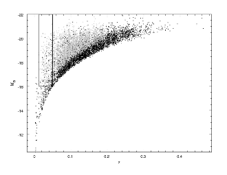
Figure 1: Absolute B band magnitude versus redshift for the MGC. Grey points denote galaxies for which the 2dFGRS $\eta$ parameter is known. The sub-sample culled consists of the grey points within the box shown, yielding 350 galaxies.

We have looked for the presence of bias in the sub-sample, which may have been introduced by selecting only those galaxies for which $\eta$ is known. We have examined the distributions of $M_{{\rm B}}$, $\mu_{{\rm B}}$, $u-r$ and Sérsic index for galaxies with and without $\eta$ within the same volume. These parameters are relatively easy to interpret and should be fairly robust. The means and standard deviations of the distributions are given in Table 3. Also listed are the biweight location and scatter estimates, which may give a truer picture of the average and scatter for a skewed distribution (see Beers et al. 1990).

A Kolmogorov-Smirnov test was performed on each pair of distributions (i.e. those with and without $\eta$) of each parameter, to test if they are consistent with being drawn from the same population. The significance of each test is given in Table 3, where a low probability indicates that it is unlikely that the two sample are drawn from the same population.

The luminosity function of galaxies in the sub-sample is shown in Figure 2. The solid histogram shows only those galaxies for which $\eta$ is known, while the dashed histogram shows the luminosity function for all galaxies within the selected volume. Overlaid is the best fitting Schechter (1976) function for the whole MGC (Driver et al. 2005). The luminosity function for the volume selected sample is consistent with that of Driver et al. (2005), indicating that the volume is representative of the MGC as a whole. The luminosity function for galaxies with $\eta$ has a lower normalisation due to the fact that some galaxies have been excluded, but the shape is consistent, except for a deficit of galaxies in the faintest bin. This indicates that the selected sub-sample is broadly representative of the whole MGC, except at the faintest magnitudes where there are too few galaxies, because the 2dFGRS, from which $\eta$ has been taken, only reaches magnitudes of $b_{{\rm j}}$=19.45 mag. This can also be seen in the top panel of Figure 3, which compares the distribution of galaxies for which $\eta$ is known to that of the excluded galaxies; the excluded galaxies are generally fainter. A Kolmogorov-Smirnov test shows that the probability is extremely small that the samples with and without $\eta$ are equivalent.

Figure 2: The luminosity function of galaxies in the selected sub-sample. The solid histogram shows only those galaxies for which $\eta$ is known, while the dashed histogram shows the luminosity function for all galaxies within the selected volume. Overlaid is the best fitting Schechter (1976) function for the whole MGC (Driver et al. 2005).

Figure 3: Distributions of $M_{{\rm B}}$, rest-frame $u-r$ colour and Sérsic index for galaxies with and without $\eta$. The galaxies without $\eta$ are preferentially faint, but have similar distributions of colour and Sérsic index.

The middle panel of Figure 3 shows the distribution of rest-frame $u-r$ colour for galaxies with and without $\eta$. The distributions appear very similar. This is reflected in the statistics listed in Table 3, and a Kolmogorov-Smirnov test shows that it is reasonable to assume that the two samples are drawn from the same parent distribution.

The bottom panel of Figure 3 shows the distribution of Sérsic index for the two groups (note there are 2 galaxies fewer in the group without $\eta$ since the surface brightness fitting produced spurious results for these galaxies). The distributions of both groups are very similar. Again the statistics are given in Table 3, and a Kolmgorov-Smirnov test shows that it is reasonable to assume that the two samples are drawn from the same parent distribution.

We also checked and found no evidence for bias in the surface brightness of the galaxies with and without $\eta$. This is at first surprising given that we are biassed against faint galaxies. However, whilst many of the excluded galaxies are faint and low surface brightness, there is a population of bright but low surface brightness galaxies which are included and hence the surface brightness distributions appear similar. Figure 4 shows histograms of the bivariate brightness distributions of the galaxies with and without $\eta$.

Figure 4: Histograms of $M_{{\rm B}}$ vs. $\mu_{{\rm B}}$ for galaxies with $\eta$ (left) and without (right).

It is expected that the colours and Sérsic indices of galaxies will approximately indicate the type of galaxy and underlying stellar populations. The lack of any significant bias in these parameters due to the exclusion of galaxies without $\eta$ suggests that the sub-sample culled provides a representative sample of galaxies within the magnitude range covered. Caution must be exercised in the interpretation of any trends in galaxy properties with magnitude however, since it is clear that the sample contains a deficit of faint galaxies.

Table 3: Means, standard deviations, biweight average ($c_{{\rm bi}}$) and scatter($s_{{\rm bi}}$), and Kolmogorov-Smirnov test significance for galaxies with and without $\eta$.

	With $\eta$ (350 galaxies)				Without $\eta$ (177 galaxies)				K-S significance
	Mean	$\sigma$	$c_{{\rm bi}}$	$s_{{\rm bi}}$	Mean	$\sigma$	$c_{{\rm bi}}$	$s_{{\rm bi}}$
$M_{{\rm B}}$	-17.81	1.10	-17.68	1.12	-17.15	1.14	-16.67	0.98	$2.8\times 10^{-13}$
rest frame $u-r$	1.74	0.57	1.70	0.57	1.67	1.07	1.59	0.56	0.24
Sérsic index	1.70	2.02	1.07	0.74	1.58	1.54	1.06	0.68	0.88
$\mu_{{\rm B}}$	22.4	1.1	22.4	1.1	22.5	1.2	22.6	1.3	0.20

3 Blue spheroids

A histogram of the rest-frame $u-r$ colours of the elliptical/lenticular galaxies is shown in Figure 5. The distribution is clearly bimodal, with $\approx 60\%$ displaying unusually blue colours for conventional ellipticals. This is strongly suggestive that there are two distinct populations of galaxies within the E/S0 class. This may be due to misclassification of the galaxies when assigning morphologies by eye, or it may be revealing a fourth category of galaxies external to the broad classes of E/S0, Sabc and Sd/Irr. However it is worth noting that if due to misclassification it occurred independently in both SCEs and SPDs samples. In order to ascertain the nature of the blue ‘ellipticals’ we have examined the distribution of several key observational quantities of the galaxies.

Figure 5: The distribution of $u-r$ colours for galaxies classified by eye as E/S0. The distribution is clearly bimodal.

The galaxies classified as elliptical/lenticular have been reassigned into red and blue classes based on a cut at $u-r=2.0$. Panels (a) and (b) of Figure 6 show the absolute $B$-band magnitude and surface brightness of the two populations versus rest-frame $u-r$. The blue galaxies are intrinsically fainter on average, with only three galaxies having $M_{{\rm B}}<-18$. This suggests the blue galaxies are less massive than the red ellipticals.

Figure 6: The properties of galaxies classified as E/S0 as a function of colour. Blue E/S0 galaxies are preferentially faint, have higher $\eta$ values indicative of ongoing star-formation and have lower Sérsic indices than conventional red early-types. The concentration and asymmetry indices are independent of colour, suggesting that the blue ellipticals are smooth systems, in contrast to conventional late-types. The vertical dashed lines indicate the colour used to define the blue spheroids. The triangles mark the locations of the example galaxies used in Figure 7.

Variations in galaxy colours can be due to variations in star-formation activity, metallicity, dust or age. However, it is unlikely that the blue population owes its colour to the presence of dust since this would make the galaxies redder than the conventional ellipticals which are known to possess very little dust.

If the blue galaxies are indeed less massive than the red population, as indicated by their $B$-band luminosities, they will have lower metallicities, since there is a well known mass-metallicity relation for galaxies (see e.g. Salzer et al. 2005 for a recent analysis). Thus the mass-metallicty relation is a plausible explanation of the variation in colour, since metal rich galaxies will appear redder. However, the bimodality cannot be due to a mass-metallicity relation for ellipticals/lenticulars only, since the variation in colour is too large (see e.g. Strateva et al. 2001 for the $u-r$ colour distribution for E/S0 galaxies in the SDSS), and the luminosity function of ellipticals is well fitted by a Schechter function (e.g. Efstathiou et al. 1988) and thus would not exhibit a bimodal colour distribution for a linear mass-metallicity relation. Thus, either the blue galaxies are not ellipticals, or there must either be variation in the age or star-formation of ellipticals as a function of mass.

Mateo (1998) shows that all dwarf galaxies in the local group have an old stellar population and most also have a young stellar population. The relative fractions of the two populations and the age of the young stellar population can have a strong effect on the galaxy colour. Hence variation in star-formation activity could potentially produce a bimodal colour distribution as observed.

The $\eta$ parameter of the 2dF survey is a sensitive indicator of star-formation activity (Madgwick et al. 2002). The two classes show a strong variation in $\eta$, panel (c) of Figure 6. The red galaxies occupy a narrow range of $\eta$ with values typical of massive early type galaxies (Madgwick 2003), whereas the blue galaxies have correspondingly larger values of $\eta$ and a larger scatter. Thus the red galaxies are mainly quiescent, but the blue galaxies display a range of star-formation activity. The correlation between colour and star-formation activity is to be expected since galaxy colour and spectra are intimately related, star-forming galaxies have stronger emission lines and display bluer colours than more quiescent galaxies (Kennicutt 1998).

Panel (d) of Figure 6 shows the Sérsic index of the galaxies when fitted with a Sérisc profile only (Graham & Driver 2005). The blue galaxies have values consistent with pure exponential systems, whereas the red galaxies have values in keeping with early-type galaxies.

Although the blue galaxies have many properties in common with late type galaxies they have similar concentration and asymmetry indices to normal ellipticals as shown in panels (e) and (f) of Figure 6, suggesting that they really are smooth systems, and not simply misclassified late-types (a comparison of $C$ with typical late types can be seen in panel (f) of Figure 8).

It seems that the blue galaxies are fundamentally different to both conventional ellipticals, spirals and late-types. Their low $B$-band luminosities suggests they are low mass systems. They have blue colours, most likely due to increased star-formation activity, as evidenced by high values of $\eta$, in common with local dwarf galaxies (Mateo 1998). We cannot rule out that they are misclassified late-type galaxies, e.g. with very low surface brightness discs, but their appearance and concentration suggests that they are smooth systems. Some examples of the appearance of these galaxies are shown in Figure 7, along with comparison images of conventional red E/S0s. Hereafter these galaxies are referred to as blue spheroids.

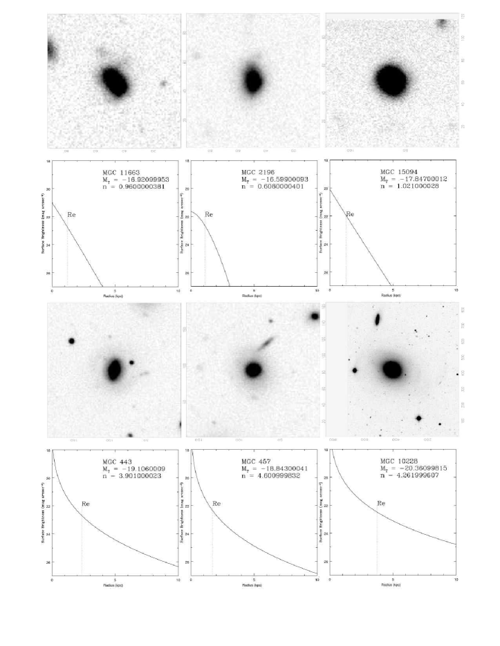
Figure 7: Examples of galaxies classified as E/S0 by eye but having much bluer colours than conventional ellipticals accompanied by their surface brightness profiles (top row). The bottom row shows conventional red E/S0 galaxies for comparison.

4 Correlations with galaxy morphology

The distribution of individual parameters as a function of morphological type has been examined. This provides an immediate understanding of the data set, useful for interpreting the more complicated statistical analyses, and as an indication of which parameters are likely to form the most useful input into clustering, principal components and discrimination analyses. The distributions of each parameter are summarised below, and examples are shown in Figure 8. Statistics of the distributions of each parameter as a function of galaxy type are given in Table 4.

4.1 $B$ band absolute magnitude

The distribution of $B$ band absolute magnitudes, $M_{{\rm B}}$, are shown in panel (a) of Figure 8. The distributions for all classes are similar with the exception of the blue spheroids, which are preferentially faint, indicating that they are less massive systems. There is a mild trend for galaxies to become fainter going from E/S0 to Sabc to Sd/Irr to blue spheroid, but it is less than 68% significant.

4.2 $B$ band surface brightness

The distribution of $B$ band surface brightness, $\mu_{{\rm B}}$, is shown in panel (b) of Figure 8. The E/S0 galaxies are generally bright, whilst the Sabc and Sd/Irr are $\sim 1.5$ mag arcsec^-2 fainter, but with a large scatter in the surface brightness of all types. The blue spheroid galaxies have a large spread in values with a peak intermediate to E/S0 and Sabcd/Irrs.

4.3 Colour

Galaxy colours have been computed using $u-r$ as Strateva et al. (2001) have shown that this combination can provide nearly optimal separation into two galaxy types for SDSS. Histograms of the colour distribution are shown in panel (c) of Figure 8.

Recall that the distinction between E/S0 and blue spheroid is artificial since blue spheroid galaxies are defined as having colours $u-r\leq 2.0$. There is a trend for galaxies to become bluer going from E/S0 to Sabc to Sd/Irr to blue spheroid, although there is a large overlap between any two adjacent classes.

4.4 2dFGRS $\eta$ parameter

Panel (d) of Figure 8 shows $\eta$ as a function of type. There is a rather clear demarcation between E/S0 galaxies and all the later types, and thus $\eta$ shows some promise of a morphological classifier. Indeed Madgwick (2003) discusses in detail the ability of $\eta$ to distinguish between early (E/S0) and late (spirals and irregulars) type galaxies. In that paper it is found that the commonly used cut of $\eta=-1.4$ compares very favourably with morphological classifications based on more complicated combinations of the first nine principal components of the spectra ($\eta$ is a linear combination of the first two).

The ability of $\eta$ to distinguish between galaxies of early and late morphologies is reasonably accomplished, however, further discrimination of different types is less robust. Panel (d) of Figure 8 shows a large degree of overlap between Sabcs, Sd/Irrs and blue spheroids. This will be shown to be a general feature throughout our attempts to provide a system of galaxy classification. It is relatively easy to separate E/S0 galaxies from Sabcd/Irrs but further distinction is extremely problematic. The comparatively large spread in $\eta$ of the spiral galaxies is also seen in the morphologically selected sample of Madgwick (2003), and in an analysis by Norberg et al. (2002) based on APM galaxies.

Madgwick et al. (2003) show that $\eta$ is much more tightly correlated with the rate of current star-formation in a galaxy (which itself may be correlated with morphology). Madgwick et al. (2002) interpret $\eta$ as a measure of the current star-formation rate in the galaxy, but they also show that $\eta$ is correlated with morphology for a sample of 21 galaxies from the Kennicutt Atlas (Kennicutt 1992). This sample classifies galaxies individually into subtypes of E/S0, Sa, Sb and Scd. It is seen that $\eta$ is progressively larger for later spiral types. Thus it could be argued that the large spread in our Sabc types seen in Figure 8 is a result of binning the sub-types Sabc into a single bin. However the rather low $\eta$ values of some Sd/Irrs and the overlap between the Sabcs and E/S0s, suggest that there is some intrinsic spread in the values of $\eta$ with sub-types (this may in part be exacerbated by fibre-placement issues. For example, it is possible that rather different $\eta$ values would result from a fibre being placed on the bulge or the disc of a spiral galaxy).

4.5 Sérsic index

The Sérsic indices, $n$, of Sabc, Sd/Irr and blue spheroid galaxies fitted with Sérsic profiles only (no exponential disc, Graham & Driver 2005) are distributed around 1, indicating an exponential surface brightness profile. On the other hand E/S0 galaxies have higher values of Sérsic index scattered around the de Vaucouleurs value of $n=4$. Panel (e) of Figure 8 shows the histograms.

4.6 Concentration and Asymmetry Indices

The concentration indices, $C$, are shown in panel (f) of Figure 8, defined as the fraction of light within 10% of the normalised radius (see Simard et al. 2002). The distribution of Sabcs is very similar to the distribution of Sd/Irrs showing an unconcentrated distribution, while the the distribution of blue spheroids is very similar to the distribution E/S0s and has higher concentration. This suggests that blue spheroids are not simply misclassified Sabcd/Irrs, and provides support for the original visual classifications.

The asymmetry indices, $A$, are similar for all classes of galaxies except Sd/Irrs which are slightly more asymmetric.

Table 4: Statistics of the distributions of key parameters as a function of galaxy type. An idea of skewness may be estimated by comparing the mean and standard deviation with the biweight estimators. For Gaussian distributions the values from each should be identical. In a heavily skewed distribution the biweight estimators are probably more useful.

	Mean	$\sigma$	$c_{{\rm bi}}$	$s_{{\rm bi}}$	Median
	$\mathbf{M_{{\rm B}}}$
E/S0	-18.32	1.13	-18.32	1.18	-18.41
Sabc	-18.07	1.09	-18.04	1.12	-18.00
Sd/Irr	-17.64	0.89	-17.57	0.91	-17.53
Blue spheroid	-16.95	0.67	-16.87	0.67	-16.78
E/S0 & blue spheroid	-17.50	1.11	-17.32	1.10	-17.25
All	-17.81	1.10	-17.74	1.12	-17.68
	$\mathbf{\mu_{{\rm B}}}$
E/S0	21.30	0.61	21.22	0.62	21.16
Sabc	22.77	0.97	22.82	1.01	22.87
Sd/Irr	22.77	0.90	22.78	0.93	22.75
Blue spheroid	22.01	0.98	21.99	1.01	22.05
E/S0 & blue spheroid	21.72	0.92	21.66	0.92	21.67
All	22.42	1.07	22.42	1.11	22.38
	$\mathbf{u-r}$
E/S0	2.46	0.22	2.46	0.22	2.47
Sabc	1.79	0.52	1.78	0.52	1.73
Sd/Irr	1.39	0.57	1.32	0.36	1.31
Blue spheroid	1.44	0.28	1.43	0.29	1.44
E/S0 & blue spheroid	1.85	0.56	1.83	0.60	1.71
All	1.74	0.57	1.70	0.57	1.63
	$\mathbf{\eta}$
E/S0	-2.10	1.05	-2.40	0.54	-2.36
Sabc	0.71	2.47	0.45	2.30	0.36
Sd/Irr	3.26	3.92	2.51	2.65	2.50
Blue spheroid	3.34	3.50	2.97	3.13	2.96
E/S0 & blue spheroid	1.14	3.86	0.69	3.63	0.45
All	1.32	3.40	0.88	2.93	0.74
	Sérsic Index
E/S0	3.49	1.48	3.52	1.55	3.68
Sabc	1.45	1.22	1.02	0.60	1.02
Sd/Irr	1.43	3.64	0.83	0.38	0.87
Blue spheroid	1.37	0.98	1.09	0.62	1.02
E/S0 & blue spheroid	2.22	1.60	1.80	1.60	1.63
All	1.70	2.03	1.07	0.74	1.07
	Concentration index (inner 10%)
E/S0	0.48	0.09	0.48	0.10	0.47
Sabc	0.28	0.11	0.26	0.10	0.26
Sd/Irr	0.27	0.13	0.24	0.09	0.24
Blue spheroid	0.41	0.13	0.40	0.13	0.42
E/S0 & blue spheroid	0.44	0.12	0.44	0.12	0.44
All	0.33	0.14	0.32	0.14	0.31
	Asymmetry index (inner 10%)
E/S0	0.06	0.03	0.05	0.03	0.05
Sabc	0.08	0.06	0.07	0.03	0.07
Sd/Irr	0.13	0.08	0.11	0.06	0.11
Blue spheroid	0.06	0.04	0.06	0.03	0.06
E/S0 & blue spheroid	0.06	0.04	0.06	0.03	0.05
All	0.08	0.07	0.07	0.04	0.07

Figure 8: Histograms of various parameters as a function of galaxy type. The median of each distribution is shown by the a dotted line. Panel (a) shows the distribution of $M_{{\rm B}}$; (b) shows the distribution of $\mu_{{\rm B}}$; (c) shows the distribution of $u-r$; (d) shows the distribution of $\eta$; (e) shows the distribution of Sersic indices; (f) shows the distribution of concentration indices.

5 Principal components analysis

The parameter set was examined in more detail by considering groupings and correlations between several parameters simultaneously. Principal components analysis (PCA, Murtagh & Heck 1987) identifies combinations of parameters which summarise the distribution of the whole set. The principal components are the projections onto the eigenvectors which successively contain the maximum variance, under the condition that all components are mutually orthogonal. This can be thought of as finding a natural set of axes throughout the parameter space which minimise the spread of the parameters. That is, if the parameters are pictured as a cloud of points in space, PCA finds the axes to which the points are closest, where closeness is defined as the Euclidean distance between vectors.

Thus PCA can be used to reduce the dimensionality of the parameter space by projecting the data onto the first few axes. Important parameters can be identified by examining the components of the eigenvectors.

5.1 Method

A good introduction to PCA is given by Murtagh & Heck (1987). The method is summarised here.

PCA takes as its input a selection of parameters from the whole catalogue. This forms an $N\times M$ matrix, ${\bf A}$, where $M$ is the number of parameters and $N$ is the number of galaxies. A new matrix, ${\bf B}$, is formed by subtracting the mean values of each parameter from every element in the matrix, and normalising by the standard deviation i.e.,

$$b_{ij}=\frac{a_{ij}-\bar{a}_{j}}{\sqrt{\frac{\sum_{i=1}^{N}\left(a_{ij}-\bar{a}_{j}\right)^{2}}{N}}}, 1\leq i\leq N, 1\leq j\leq M$$ (1)

where $b_{ij}$ are the elements of ${\bf B}$ and $a_{ij}$ are the elements of ${\bf A}$ and

$$\bar{a}_{j}=\frac{1}{N}\sum_{i=1}^{N}a_{ij}.$$ (2)

The covariance matrix of ${\bf B}$ is then formed,

$$c_{jk}=\frac{1}{N}\sum_{i=1}^{N}b_{ij}b_{ik}, 1\leq j\leq M, 1\leq k\leq M$$ (3)

where $c_{jk}$ are the elements of the covariance matrix ${\bf C}$. Matrix ${\bf C}$ is real and symmetric, and therefore has real, positive eigenvalues. The numerical order of these eigenvalues yields the strength of the variance of the data in the corresponding eigenvector.

The principal components, ${\bf P}$, can then be found by projecting the eigenvectors onto the normalised, mean-subtracted matrix ${\bf B}$, i.e.

$${\bf P}={\bf BC}.$$ (4)

The order of the principal components is found from the numerical order of their corresponding eigenvalues, so $pc1$ are the elements of the $N\times 1$ column vector corresponding to the highest eigenvalue, etc.

5.2 Results

A PCA was carried out on various combinations of the parameters $\{M_{{\rm B}},\mu_{{\rm B}},u-r,\eta,n,C,A\}$ in order to determine any particular combinations of parameters which account for a large amount of variance, and hence provide a useful description of galaxy properties.

Many combinations of parameters were experimented with. In no experiment did any individual parameter dominate the principal eigenvectors: no single parameter had significantly more variance than any other. Considering the parameters as a cloud of points, they are not elongated in any way which is aligned to an individual parameter. Compression of the data required several parameters to be combined together, indicating that photometric ($M_{{\rm B}}$, $\mu_{{\rm B}}$, $u-r$), spectroscopic ($\eta$) and structural ($n$, $C$, $A$) parameters are all of similar importance in describing the distribution of galaxies throughout the parameter space.

The first principal component usually projected the galaxies in such a way that the E/S0 galaxies were separated from the other types of galaxies. Thus, the parameter space has a maximum variance in a direction that separates E/S0 galaxies from other types. Note that PCA is not given any information regarding the visual morphological classifications. The distinction between E/S0 and other galaxies is clearly of fundamental importance in terms of their observational properties; influencing photometric, spectroscopic and structural parameters. Two examples of this are shown in Figure 9 using the subsets $\{M_{{\rm B}},\mu_{{\rm B}},u-r,\eta,n,C,A\}$ and $\{u-r,\eta,n,C\}$, illustrating the distinction between E/S0 and the other galaxies. Note that the distribution of Sabcs is skewed with a tail overlapping with the E/S0s. Whilst we cannot rule out misclassification for all the Sabc galaxies in the tail, some of them display very clear spiral arms. The other principal components showed no clear distinction between galaxies of different types. No combination of principal components was found which could separate Sabc, Sd/Irr and blue spheroid galaxies.

Figure 9: The distribution of the first principal component, $pc1$, for galaxies of different type. The top panel shows the results of PCA using the set $\{M_{{\rm B}},\mu_{{\rm B}},u-r,\eta,n,C,A\}$, and the bottom panel using the set $\{u-r,\eta,n,C\}$ . In both cases the first principal component clearly separates early and late type galaxies.

A caveat is to note that information on the errors associated with the parameters was not included in the analysis, since errors are not known for all parameters, e.g. $\eta$. If some parameters have large errors associated with them they may skew the results.

6 Linear discriminant analysis

Linear discriminant analysis (LDA) defines combinations of parameters which optimally discriminate between objects of known classes. We have used LDA with various combinations of parameters to discriminate between galaxies of different morphology. Thus we can assess the relative merit of the input parameters in assigning, and hence correlation with, galaxy morphology.

6.1 Method

Consider again the $N\times M$ matrix ${\bf B}$ of equation 1, containing the normalised, mean subtracted properties of a sample of galaxies, where $N$ is the number of galaxies and $M$ is the number of measured properties. Assuming that the sample has been divided into two classes, 0 and 1, the vectors, ${\bf m_{0}}$ and ${\bf m_{1}}$, describing the means of each property, and the covariance matrices, ${\bf V_{0}}$ and ${\bf V_{1}}$, of each class may be calculated.

The combined covariance matrix, ${\bf W}$, of each class may then be computed,

$${\bf W}={\bf V}_{0}+{\bf V}_{1}.$$ (5)

Fisher’s linear discriminant is defined such as to maximise the distance between the samples means after standardising by the variance within the samples (Hand 1981, page 83). That is, we want to maximise the ratio,

$$\frac{{\bf m_{0}}-{\bf m_{1}}}{{\bf Wf}},$$ (6)

where ${\bf f}$ is a vector describing the set of weights which maximise equation 6. Thus,

$${\bf f}\propto{\bf W}^{-1}({\bf m_{0}}-{\bf m_{1}}).$$ (7)

Finally we may define a new vector containing the initial input data weighted so as to maximise the difference between class 0 and 1,

$${\bf t}=({\bf m_{{\rm 0}}}-{\bf m_{{\rm 1}}})^{{\rm T}}{\bf W}^{-1}{\bf B}.$$ (8)

Thus Fisher’s LDA must first be applied to a population of galaxies whose types are known (in our case this is the whole catalogue). Thereafter an appropriate division can be made based on a value of $t$ (where $t_{i}$ are the elements of vector ${\bf t}$). The choice of $t$ will depend on how ‘pure’ a sample is desired, setting $t$ to give little contamination in one class, will give a larger contamination in the other class if the two classes overlap.

6.2 Results

The data were first standardised to zero mean and unit variance before performing the analysis. We experimented with various combinations of parameters. It was relatively easy to separate E/S0s and the rest. Discriminating between other types of galaxies was always less successful. Some examples are given below.

The input set $\{M_{{\rm B}},\mu_{{\rm B}},u-r,\eta,n,C,A\}$ was used. The resulting discrimination is illustrated in Figure 10. A cut at $t(x)=2.40$ resulted in 93% of E/S0s being correctly assigned and 93% of others. This same cut correctly classified 99% of galaxies below the cut and 66% above. Thus, the separation of E/S0 from the rest of the galaxies was relatively successful cf. 80% agreement when classifying by eye.

In contrast Sabcs could only be separated with $72\%$ success, Sd/Irrs with $75\%$ success and blue spheroids with $81\%$ success.

Figure 10: Example of linear discriminant analysis. The closely hashed histogram on the right hand side represents E/S0 galaxies and the open hashed histogram the rest. A cut at $t(x)=2.40$ correctly classifies 92% of E/S0 galaxies.

An input set consisting of purely structural parameters $\{n,C,A\}$ was experimented with. This was less successful than the full parameter set, but E/S0s could still be separated with 83% success.

Similarly star-forming parameters $\{\eta$, $u-r\}$ were investigated. These two parameters alone could separate E/S0 galaxies with 88% success, but had poorer success rates at separating any other types of galaxies.

7 Clustering Analysis

So far the work presented has concentrated mainly on correlations with the morphological types assigned by eye, and combinations of parameters to optimise discrimination between these a priori defined classes. It may be the case however, that there are natural classes of objects grouped within the parameter space which do not necessarily reflect morphological types. A hierarchical clustering analysis (HCA) has been performed in order to search for such natural groupings within the parameter set. The method and the results are described below.

7.1 Method

$N$ galaxies, each described by $M$ parameters, are described by matrix $\bf{A}$, as in PCA. Each galaxy can be thought of as a point in a parameter space. The distance between each point and all the others is calculated yielding a set of $N(N-1)/2$ distances, where the distance will be defined below. Once the distances are known clusters are made by agglomerating points within the parameter space based on their distances. For example, the smallest distance $d_{ik}$ is determined, and objects $i$ and $k$ are then agglomerated and replaced with a new object $i\cup k$. The set of distances are then updated using the new object in place of $i$ and $k$.

Several methods can be used to define distances, and the centres of the newly created clusters. The method used here is that of Ward (1963), which defines the distance between two clusters as the amount by which the total distance from each point to the centre of its cluster would increase by merging the two clusters (technically, it is the sum of the squares of the Euclidean distances from the objects to the joint cluster mean minus the sum of squares from the objects to their individual cluster means, so the distance is the amount the sum of squares would increase if the clusters were to be merged, see Hand 1981). This method was implemented using freely available java software written by F. Murtagh.

7.2 Results

Again experiments were performed with the input set $\{M_{{\rm B}},\mu_{{\rm B}},u-r,\eta,n,C,A\}$, and parameters were standardised on input. Galaxies were split into only two clearly distinct classes.

Classifying galaxies into two categories which gave the greatest separation, reveals a segregation of galaxies strongly dependent on $u-r$, $\eta$ and the Sersic index, $n$. Classification into more than two categories did not reveal any strong trends with any parameter for the third class of object. Figure 11 shows the dependence of the two natural classes on $u-r$, $\eta$ and $n$.

Figure 11: Galaxies classified into natural categories as a function of rest-frame $u-r$, Sérsic index and $\eta$.

The clustering of the galaxies in these natural classes was tested for correlations with morphology. Membership of group 1 or 2 was assigned as an extra input parameter into a LDA. No improvement (or deterioration) was made over previous efforts to discriminate galaxies into known morphological types. This indicates that the classes defined from hierarchical clustering are no more closely correlated with morphology than the input parameters, although this could be due to poor classification of galaxies when assigning types by eye. Figure 12 shows the distribution of each morphological type within the clusters. One cluster is made almost solely of E/S0 galaxies with the majority of all other types occupying the other cluster. Although it is possible that some of the galaxies in class 2 of Figure 12 were originally classified as Sabcd/Irr/blue spheroid as a result of misclassification, some of them have definite spiral morphology.

Figure 12: The distribution of galaxies within each cluster per morphological type.

Using the same input parameters LDA could reproduce the classifications of the hierarchical clustering analysis with excellent success of 95% (with 98% of galaxies below the cut, and 84% above correctly classified), showing that there is little overlap between the two classes in this parameter space.

8 Discussion

We have examined the distributions of photometric ($M_{{\rm B}}$, $\mu_{{\rm B}}$, $u-r$), spectral ($\eta$) and structural ($n$, $C$, $A$) parameters from a well defined sample of nearby galaxies culled from the Millennium Galaxy Catalogue. Galaxies were classified into broad morphological types by visual inspection.

8.1 Blue spheroids

A significant fraction of galaxies classified as ellipticals were found to have some properties (colour, $\eta$ and $n$) more in keeping with late-type galaxies, but with concentration and asymmetry indices more typical of early-type galaxies. These galaxies are preferentially faint, suggesting that they are low mass galaxies. A significant fraction of these galaxies appear to be undergoing significant star-formation. Such blue spheroids have previously been reported elsewhere, e.g. in studies of faint field galaxies in HST images (Driver et al. 1995). This population of blue spheroids may well be responsible for the highly discrepant “early-type” luminosity function estimates (see de Lapparent 2003 for discussion). Early-types cuts by colour or spectral type will exclude this population whereas morphological cuts will not. Note also that the high fraction of blue spheroids in our sample is probably a result of the near volume-limited nature of the sample, the fraction would likely be much lower in a magnitude limited sample.

According to hierarchical theories of structure formation, less massive galaxies form at earlier epochs than massive galaxies. This leads to the conclusion that the stellar populations of massive galaxies should be younger than those of dwarf galaxies, unless star-formation is not coincident with the epoch of galaxy assembly. Observationally, however, there is a lot of evidence that less massive galaxies undergo star-formation at later epochs than massive galaxies. Local dwarf galaxies are seen to be composed of significant fractions of young stars, perhaps predominantly so (Mateo 1998). Less massive galaxies are more likely to have undergone recent star-bursts than massive galaxies (Cowie et al. 1996; Gavazzi et al. 1996; Kauffmann et al. 2003). The colour-magnitude relation of galaxies in groups at high redshift shows a truncation at the faint end, beyond which the typical red galaxies are supplanted by a blue population (Kodama et al. 2004; De Lucia et al. 2004). Similarly, De Propris et al. (2003) shows that the increased fraction of blue galaxies in clusters at high redshift (e.g. Butcher & Oemler 1984) may be driven by low mass galaxies which have recently undergone star-formation.

The blue spheroid galaxies found in the present study are consistent with this picture of down-sizing in galaxy formation. The galaxies are centrally concentrated, smooth, and appear as normal ellipticals, suggesting they have not undergone any recent mergers which could trigger star-formation, but they possess colours and $\eta$ values characteristic of star-forming galaxies. Finally it is worth noting that the statistical tools were unable to isolate the blue spheroid population from the late types. However the eyeball classifications did. This implies that there is additional useful information that can be measured. This might include smoothness (e.g., CAS analysis; Conselice 2003) or low frequency Fourier modes (e.g., Odewahn et al. 2002 for example).

8.2 Classification and discrimination of galaxy types

The over-riding feature of all the multi-variate statistical studies was the existence of just two clear groups of galaxies (albeit with some overlap in their properties), corresponding to early types (E/S0) and the rest (Sabcd/Irr/blue spheroid). The physical difference being the colour, profile shape and the amount of star-formation activity. Further distinction of separate groups was always less convincing.

The class of galaxies comprised of Sabcd/Irr/blue spheroids is distributed remarkably smoothly throughout the parameter space, and distinction between any of the morphological types based on their global photometric, spectral and structural properties is difficult and unconvincing. This is not to say there are no correlations of galaxy properties with morphology. For example, Roberts & Haynes (1994) find correlations (notwithstanding large dispersions) with Hubble type and average values of total mass, mass fraction of neutral hydrogen, total surface density and integrated galaxy colour, amongst others. These correlations are easily understood in terms of variation in star-formation activity as a function of morphology. However, the transition of properties from spiral to irregular galaxies is always smooth, in keeping with their occupation of a single class, and results largely from the variation in mass along the sequence. On the other hand there can be large discontinuities between the properties of elliptical and spiral galaxies, e.g. HI mass fraction.

It is plausible then, that the astrophysical processes governing the formation and evolution of galaxies are the same for all morphological types, Sa to Irr, with minor variations due to different masses of the galaxies, e.g. the colour differences can be qualitatively explained by the relation between mass and metallicity. Ellipticals and lenticulars however, appear to require different astrophysical processes.

The real and fundamental separation of these two groups needs to be understood in the context of galaxy evolution. The existence of two distinct groups can be explained either in terms of evolution of galaxies or in terms of initial conditions.

Perhaps the simplest explanation is that the difference is a result of initial conditions, with the two types of galaxies having different formation mechanisms. This requires that ellipticals collapsed early in a dissipationless manner, and hence contain old stellar populations and a three-dimensional appearance. Spirals collapsed dissipatively, and hence formed into a disc with a reservoir of gas. The difficulty in this case lies in explaining what causes galaxies to collapse in different ways. Also this idea is at odds with the cold dark matter paradigm, which predicts that galaxies assemble in a hierarchical manner, through a series of mergers (Baugh et al. 1996).

Hubble (1936) proposed that the morphological sequence of galaxies represents an evolution from the simple elliptical forms to the grand design of Sc galaxies. Much modern research proposes morphological evolution in the opposite direction, with merging discs forming large ellipticals (see e.g. Schweizer 2000 for a review). Reconciliation between two clearly distinct classes of galaxies, both in terms of appearance and stellar population, with a transformation between the two classes suggests that any such transformations are rapid, or occurred at early times, in order to account for the relatively few galaxies with intermediate properties, e.g., as in  Figure 9.

Numerical simulations show that the transformation from two disc galaxies to a single merged remnant can occur in about 1.5 rotation periods of the input discs, corresponding to $\sim$400Myr for galaxies the size of the Milky Way (Schweizer 2000), suggesting that morphological transformations may indeed be fast enough to preserve a bimodal population of galaxies.

Balogh et al. (2004) investigate the transformation of galaxy colour as a function of environment, finding similarly bimodal distributions. Using Bruzual & Charlot (2003) synthetic stellar population models, they show that if star-formation is ceased abruptly then galaxy colours transform on the short time-scale of 750Myr. If however, star-formation decays with an exponential time-scale of 2Gyr, as expected for a process such as strangulation, they show that colours are transformed over a period of 4Gyr.

Note that, for massive cluster galaxies at least, morphological transformation must take place at a slower rate than transformation in star-formation rate, to account for the existence of a tight colour-magnitude relation for luminous early-type galaxies to high redshift (Stanford et al. 1998; Holden et al. 2004), otherwise, at some redshift there would exist a population of bright blue elliptical galaxies which are not observed. Note also that from our visual classifications we see very few such bright blue ellipticals, but we do observe apparently quiescent spirals and faint blue spheroids. Thus transformation of the stellar populations in massive cluster galaxies must be occurring faster than $\sim 400$Myr if transformations are occurring at $z<1$.

Thus the bimodality of the galaxy populations could be due to rapid transformation of both stellar-population and morphology, although physically motivated mechanisms such as strangulation occur at slower rates (Larson et al. 1980; Balogh et al. 2000).

The bimodality could be produced through slower transformations, if they occur mainly at high redshift. There is indeed some evidence that this is the case. van Dokkum et al. (1999) finds a high rate of interaction between galaxies in the $z=0.83$ cluster MS1054-0 3. There is a close link between mergers, ultra-luminous infrared galaxies and quasars which suggests that the major epoch of merging occurred coincidentally with the peak in quasar activity, around $z\approx 2$ (Schweizer 2000). Bundy et al. (2005) present evidence that morphological transformations of lower mass galaxies may take place at later cosmic epochs, which may explain why the majority of blue spheroids we see are low mass systems.

Note also that the major-merger rate, as measured in the MGC, is low (De Propris et al. 2005), strongly suggesting that transformations as a result of mergers will not be very common today. Also, Le Fèvre et al. (2000) see a strong increase in the fraction of major-mergers as a function of redshift in the Canada-France Redshift Survey.

These results suggest that the distinction between the two classes of galaxies is a result of the high redshift of the merging and transformation of galaxies. We note however, that lack of merging at low redshifts is somewhat at odds with predictions of CDM, in which approximately 50% of galaxies should have undergone a major merger since $z=1$ (Murali et al. 2002).

We postulate that a similar study of a high redshift sample of galaxies, should produce different results and a blurring of the two groups as the redshift of transformations and mergers is reached, if transformations do indeed occur slowly at high redshift.

Finally we note that an analysis of the results of bulge-disc decomposition and CAS (Conselice 2003) analysis of the galaxies are in progress and will be presented in future papers.

References

- Abazajian et al. (2003) Abazajian, K., et al. 2003, AJ, 126, 2081
- Abazajian et al. (2005) Abazajian, K., et al. 2005, AJ, 625, 613
- Abraham et al. (1996) Abraham, R. G., van den Bergh, S., Glazebrook, K., Ellis, R. S., Santiago, B. X., Surma, P., Griffiths, R. E. 1996, ApJS, 107, 1
- Balogh et al. (2004) Balogh, M. L., Baldry, I. K., Nichol, R., Miller, C., Bower, R., Glazebrook, K. 2004, ApJ, 615, L101
- Balogh et al. (2000) Balogh, M. L., Navarro, J. F., Morris, S. L. 2000, ApJ, 540, 113
- Baugh et al. (1996) Baugh, C. M., Cole, S., Frenk, C. S. 1996, MNRAS, 283, 1361
- Beers et al. (1990) Beers, T. C., Flynn, K., Gebhardt, K. 1990, AJ, 100, 32
- Bell et al. (2004) Bell, E. F., et al. 2004, ApJ, 608, 752
- Binney & Merrifield (1998) Binney, J., Merrifield, M. 1998, Galactic astronomy (Princeton University Press)
- Bruzual & Charlot (2003) Bruzual, G., Charlot, S. 2003, MNRAS, 344, 1000
- Bundy et al. (2005) Bundy, K., Ellis, R. S., Conselice, C. J. 2005, ApJ, 625, 621
- Butcher & Oemler (1984) Butcher, H., Oemler, A. 1984, ApJ, 285, 426
- Colless et al. (2001) Colless, M., et al. 2001, MNRAS, 328, 1039
- Conselice (2003) Conselice, C. J. 2003, ApJS, 147, 1
- Cowie et al. (1996) Cowie, L. L., Songaila, A., M., H. E., Cohen, J. G. 1996, AJ, 112, 839
- Cross et al. (2004) Cross, N. J. G., Driver, S. P., Liske, J., Lemon, D. J., Peacock, J. A., Cole, S., Norberg, P., Sutherland, W. J. 2004, MNRAS, 349, 576
- Croton et al. (2005) Croton, D. J., et al. 2005, MNRAS, 356, 1155
- de Lapparent (2003) de Lapparent, V. 2003, A&A, 408, 845
- De Lucia et al. (2004) De Lucia, G., et al. 2004, ApJ, 610, L77
- De Propris et al. (2005) De Propris, R., Liske, J., Driver, S., Allen, P., Cross, N. 2005, ApJ, in press
- De Propris et al. (2003) De Propris, R., Stanford, S. A., Eisenhardt, P. R., Dickinson, M. 2003, ApJ, 598, 20
- De Propris et al. (2004) De Propris, R., et al. 2004, MNRAS, 351, 125
- Dressler (1980) Dressler, A. 1980, ApJ, 236, 351
- Dressler et al. (1997) Dressler, A., et al. 1997, apj, 490, 577
- Driver et al. (2005) Driver, S., Liske, J., Cross, N., De Propris, R., Allen, P. 2005, MNRAS, 360, 81
- Driver et al. (1995) Driver, S. P., Windhorst, R. A., Griffiths, R. E. 1995, ApJ, 453, 48
- Efstathiou et al. (1988) Efstathiou, G., Ellis, R. S., Peterson, B. A. 1988, MNRAS, 232, 431
- Gavazzi et al. (1996) Gavazzi, G., Pierini, D., Boselli, A. 1996, A&A, 312, 397
- Graham & Driver (2005) Graham, A. W., Driver, S. W. 2005, PASA, 22(2), 118
- Hand (1981) Hand, D. 1981, Discrimination and Classification (John Wiley and Sons Ltd.)
- Hogg et al. (2004) Hogg, D. W., et al. 2004, ApJ, 601, L29
- Holden et al. (2004) Holden, B. P., Stanford, S. A., Eisenhardt, P., Dickinson, M. 2004, AJ, 127, 2484
- Hubble (1936) Hubble, E. P. 1936, Realm of the Nebulae (Yale University Press)
- Kauffmann et al. (2003) Kauffmann, G., et al. 2003, MNRAS, 341, 54
- Kennicutt (1992) Kennicutt, R. C. 1992, ApJS, 79, 255
- Kennicutt (1998) Kennicutt, R. C. 1998, ARA&A, 36, 189
- Kodama et al. (2001) Kodama, T., Smail, I., Nakata, F., Okamura, S., Bower, R. G. 2001, ApJ, 562, L9
- Kodama et al. (2004) Kodama, T., et al. 2004, MNRAS, 350, 1005
- Kron (1980) Kron, R. 1980, ApJS, 305
- Larson et al. (1980) Larson, R. B., Tinsley, B. M., Caldwell, C. N. 1980, ApJ, 237, 692
- Le Fèvre et al. (2000) Le Fèvre, O., et al. 2000, MNRAS, 311, 565
- Lewis et al. (2002) Lewis, I., et al. 2002, MNRAS, 334, 673
- Liske et al. (2003) Liske, J., Lemon, D. J., Driver, S. P., Cross, N. J. G., Couch, W. J. 2003, MNRAS, 344, 307
- Madgwick (2003) Madgwick, D. S. 2003, MNRAS, 338, 197
- Madgwick et al. (2003) Madgwick, D. S., Somerville, R., Lahav, O., Ellis, R. 2003, MNRAS, 343, 871
- Madgwick et al. (2002) Madgwick, D. S., et al. 2002, MNRAS, 333, 133
- Mateo (1998) Mateo, M. 1998, ARA&A, 36, 435
- Murali et al. (2002) Murali, C., Katz, N., Hernquist, L., Weinberg, D. H., Davé, R. 2002, ApJ, 571, 1
- Murtagh & Heck (1987) Murtagh, F., Heck, A. 1987, Multivariate data analysis (Astrophysics and Space Science Library, Dordrecht: Reidel, 1987)
- Norberg et al. (2002) Norberg, P., et al. 2002, MNRAS, 332, 827
- Odewahn et al. (2002) Odewahn, S. C., Cohen, S. H., Windhorst, R. A., Philip, N. S. 2002, ApJ, 568, 539
- Poggianti (1998) Poggianti, B. M. 1998, in ASP Conf. Ser. 146: The Young Universe: Galaxy Formation and Evolution at Intermediate and High Redshift, 452
- Roberts & Haynes (1994) Roberts, M. S., Haynes, M. P. 1994, ARA&A, 32, 115
- Salzer et al. (2005) Salzer, J., Lee, J., Melbourne, J., Jangren, A. 2005, ApJ, in press
- Schechter (1976) Schechter, P. 1976, ApJ, 203, 297
- Schweizer (2000) Schweizer, F. 2000, Philosophical Transactions: Mathematical, Physical & Engineering Sciences, 358, 2063
- Simard (1998) Simard, L. 1998, in ASP Conf. Ser. 145: Astronomical Data Analysis Software and Systems VII, 108
- Simard et al. (2002) Simard, L., et al. 2002, ApJS, 142, 1
- Stanford et al. (1998) Stanford, S. A., Eisenhardt, P. R., Dickinson, M. 1998, ApJ, 492, 461
- Strateva et al. (2001) Strateva, I., et al. 2001, AJ, 122, 1861
- van Dokkum et al. (1999) van Dokkum, P. G., Franx, M., Fabricant, D., Kelson, D. D., Illingworth, G. D. 1999, ApJ, 520, L95
- Ward (1963) Ward, J. H. 1963, JASA, 58, 236
- Whitmore et al. (1993) Whitmore, B. C., Gilmore, D. M., Jones, C. 1993, ApJ, 407, 489