Dynamics of the Inflationary Flow Equations

Abstract

We present a dynamical analysis of the inflationary flow equations. Our technique uses the Hubble ‘jerk’ parameter $\xi\equiv(m_{\mbox{\scriptsize{Pl}}}^{4}/16\pi^{2})H^{-2}(dH/d\phi d^{3}H/d\phi^{3})$ (where $H$ is the Hubble parameter and $\phi$ the inflaton) as a discriminant of stability of fixed points. The results of the analysis are used to explain qualitatively the distribution of various observable parameters (e.g. the tensor-scalar ratio, $r$, and scalar spectral index, $n_{s}$) seen in numerical solutions of the flow equations using stochastic initial conditions. Finally, we give a physical interpretation of the flow in phase-space in terms of slow-roll motion of the inflaton.

I Introduction

Since the first discussions of inflationary cosmology more than twenty years ago, a huge number of specific models have been proposed. Most of these are ‘phenomenological’, though increasing effort has been invested towards constructing physically motivated models such as brane inflation (for reviews, see lr ; que ). Given a plethora of models, one can ask whether aspects of inflation can be studied without recourse to particular scenarios.

Hoffman and Turner ht first addressed this by introducing flow equations that govern evolution of observables in any single-field model of inflation. These flow equations were later generalised to arbitrary order by Kinney kin . In his notation, the inflationary flow equations are :

$${d\epsilon\over dN} = \epsilon(\sigma+2\epsilon)\phantom{t},$$

$${d\sigma\over dN} = -\epsilon(5\sigma+12\epsilon)+2(\phantom{t}^{2}\lambda_{H})\phantom{t},$$ (1)

$${d\over dN}\phantom{t}^{\ell}\lambda_{H} = \Big{[}{\ell-1\over 2}\sigma+(\ell-2)\epsilon\Big{]}\phantom{t}^{\ell}\lambda_{H}+\phantom{t}^{\ell+1}\lambda_{H}\phantom{t}.\phantom{t}(\ell\geq 2)$$

Here the derivative with respect to the number of e-folds, $N$, runs in the opposite direction to time. The flow equations represent an infinite dimensional dynamical system of the following parameters given in terms of the Hubble parameter $H(\phi)$:

$$\epsilon \equiv {m_{\mbox{\scriptsize{Pl}}}^{2}\over 4\pi}\bigg{(}{H^{\prime}\over H}\bigg{)}^{2},$$

$$\eta \equiv {m_{\mbox{\scriptsize{Pl}}}^{2}\over 4\pi}\bigg{(}{H^{\prime\prime}\over H}\bigg{)}\phantom{t},$$

$$\phantom{t}{}^{\ell}\lambda_{H} \equiv \bigg{(}{m_{\mbox{\scriptsize{Pl}}}^{2}\over 4\pi}\bigg{)}^{\ell}{(H^{\prime})^{\ell-1}\over H^{\ell}}{d^{\ell+1}H\over d^{\ell+1}\phi}\phantom{t},$$ (2)

$$\sigma \equiv 2\eta-4\epsilon\phantom{t},$$

where $m_{\mbox{\scriptsize{Pl}}}$ is the Planck mass and primes denote derivatives with respect to the inflaton $\phi$. The flow parameters $\{\epsilon,\sigma,^{\ell}\lambda_{H}\}$ are related to the conventional slow-roll parameters lid

$$\epsilon_{V}={m_{\mbox{\scriptsize{Pl}}}^{2}\over 16\pi}\Big{(}{V^{\prime}\over V}\Big{)}^{2}\phantom{t},\qquad\eta_{V}={m_{\mbox{\scriptsize{Pl}}}^{2}\over 8\pi}\Big{(}{V^{\prime\prime}\over V}\Big{)}\phantom{t},$$ (3)

etc. defined in terms of derivatives of the inflaton potential $V(\phi)$. The validity of the slow-roll approximation is more easily expressed in terms of these parameters than those of equation (2). The relationship between the two sets of parameters is discussed in §3.

Solving the flow equations gives $\epsilon(\phi)$ or, equivalently, $H(\phi)$. These in turn fix the shape of potential $V(\phi)$ via the Hamilton-Jacobi equation

$$\big{(}H^{\prime}(\phi)\big{)}^{2}-{12\pi\over m_{\mbox{\scriptsize{Pl}}}^{2}}H^{2}(\phi)=-{32\pi^{2}\over m_{\mbox{\scriptsize{Pl}}}^{4}}V(\phi)\phantom{t},$$ (4)

which is equivalent to the Friedmann ‘acceleration’ equation

$${\ddot{a}\over a}={H^{2}(\phi)}\Big{(}1-\epsilon\Big{)}\phantom{t}.$$ (5)

From (5), it is clear that inflation is sustained as long as $\epsilon<1$. Recently, Liddle lidd showed that an analytic solution to the flow equations, closed at some order, yields a potential $V(\phi)$ expanded as a rational polynomial.

Using the flow equations, a large number of numerically viable inflationary models can be readily produced stochastically. However, a mathematical analysis of the flow equations - an infinite hierarchy of differential equations - appears daunting. While there have been discussions of ‘attractor’ solutions kin ; eak in the past, in this paper we present a more rigorous analysis of the flow equations. We begin by exploring the dynamics in the phase-space of flow parameters $\{\epsilon,\sigma,^{\ell}\lambda_{H}\}$ and classifying all trajectories. In particular, we are able to explain the complicated motions in the $(\sigma,\epsilon)$ plane as observed in kin ; eak . We then analyse how these motions translate to structures in the space of observables. Finally, we discuss the physical implications of our analysis when the Hamilton-Jacobi equation is incorporated.

II Phase-space dynamics

II.1 The nature of fixed-points

Two sets of fixed points of the flow equations are evident from inspection:

• ${\epsilon=0,\phantom{t}\sigma=}$ constant- so called ‘${r=0}$’ fixed points, from the fact that the tensor-scalar ratio $r\propto\epsilon$ vanishes along that line.

• ${\epsilon>0,\phantom{t}\sigma=-2\epsilon,\phantom{t}^{\ell+1}\lambda_{H}=\epsilon(\phantom{t}^{\ell}\lambda_{H})}$- so called ‘power-law’ fixed point, being a feature of power-law inflation from a potential such as $V(\phi)\propto\exp\big{(}-\sqrt{8\pi}\phi/m_{\mbox{\scriptsize{Pl}}}\big{)}$.

As a starting point, let us examine the nature of these fixed points in the simplest two-dimensional projected phase-space.

II.1.1 Simplest $(\sigma,\epsilon)$ dynamics

Consider the two lowest order equations in the system (2). The dynamics in the $(\sigma,\epsilon)$ phase-space clearly depend on the value of $\phantom{t}{}^{2}\lambda_{H}$, the Hubble ‘jerk’ parameter. Following the notation of p03 , we shall rewrite it as

$$\xi \equiv \phantom{t}{}^{2}\lambda_{H}\equiv{m_{\mbox{\scriptsize{Pl}}}^{4}\over 16\pi^{2}}\bigg{(}{H^{\prime}H^{\prime\prime\prime}\over H^{2}}\bigg{)}\phantom{t}.$$ (6)

Thus we are examining the dynamics of the two-dimensional system

$${d\epsilon\over dN} = \epsilon(\sigma+2\epsilon)\phantom{t},$$ (7)

$${d\sigma\over dN} = -\epsilon(5\sigma+12\epsilon)+2\xi\phantom{t}.$$ (8)

The fixed points in the $(\sigma,\epsilon)$ system are easy to analyse if $\xi$ is treated, for now, as a constant. By linearising (7) and (8), one sees that the sign of $\xi$ discriminates the stability of fixed points in the $(\sigma,\epsilon)$ plane. The results of a standard fixed point analysis is shown in Table I.

We draw attention to the ‘nullclines’ where the flow becomes vertical or horizontal:

Horizontal nullcline $$: \quad\sigma=-2\epsilon\phantom{t},$$ (9)

Vertical nullcline $$: \quad\epsilon^{2}+{5\over 12}\sigma\epsilon={\xi\over 6}\phantom{t}.$$ (10)

These curves provide useful demarcations of where flows change direction, and we include them in our phase portraits.

II.1.2 Methodology

Inflation can be investigated ‘stochastically’ by first selecting a random point in the flow parameter space as an initial configuration of a particular universe. Because this is not the same as assigning randomness to initial conditions for inflation, we adhere to the phrase ‘initial configuration’ to keep this distinction clear.

An initial configuration is then evolved forward in time (backward in e-fold) until inflation ends in one of the following plausible ways:

1. By achieving $\epsilon=1$. When this happens, we say for convenience that the ‘slow-roll’ condition has been violated (keeping in mind that inflation ends because equation (5) changes sign rather than because the slow-roll parameters $\epsilon_{V}$ and $|\eta_{V}|$ of equation (3) exceed unity). Observables are then calculated a specific number of e-folds (which we take to be $55$, unless otherwise stated) before the end of inflation by integrating backward in time. This choice is in accordance with analyses of references leach ; dod which indicate that for plausible assumptions concerning reheating etc, the observable perturbations were generated 50 to 60 e-folds before the end of inflation. Variation of this number is explored in §2.

2. By an abrupt termination, perhaps from intervention of an auxiliary field in hybrid inflation lr , or when open strings become tachyonic in brane inflation que . Because these scenarios accommodate large number of e-folds during inflation, one identifies them with an asymptotic behaviour of a trajectory. Observables are calculated along the asymptote. We return to the practical issues of calculating observables later.

Because we evolve flows backward in e-fold, the notions of stability and attraction found in Table I become reversed. This is summarised in Table II, from which we conclude that given an initial configuration in $\{\epsilon,\sigma,^{\ell}\lambda_{H}\}$ space, as long as the function:

$$\mbox{sgn}(\xi)=\begin{cases}\phantom{t}\phantom{t}1\quad\mbox{if}\phantom{t}\xi>0\phantom{t},\\ \phantom{t}\phantom{t}0\quad\mbox{if}\phantom{t}\xi=0\phantom{t},\\ -1\quad\mbox{if}\phantom{t}\xi<0\phantom{t},\end{cases}$$

remains constant, then the dynamics in the $\{\epsilon,\sigma,^{\ell}\lambda_{H}\}$ phase-space are completely characterized.

II.1.3 Dynamics of $\xi$

Having assumed that $\xi$ was constant, we can now incorporate aspects of the dynamics of $\xi$ using the function $\mbox{sgn}(\xi)$. If $\mbox{sgn}(\xi)$ changes unpredictably, then the classification in Table II would be useless. We now show that this is not the case.

Starting from equation (2), one finds that the evolution of $\xi$ has no explicit dependence on $\epsilon$

$${d\xi\over dN}=-{1\over 2}\sigma\xi+\phantom{t}^{3}\lambda_{H}\phantom{t}.$$ (11)

The solution of equation (11) is :

$$\xi(N)=\xi(N_{0})\exp\Big{(}{1\over 2}\int_{N_{0}}^{N}{\sigma(n)}dn\Big{)}\qquad\qquad$$

$$\quad\quad+\int_{N_{0}}^{N}\phantom{t}{}^{3}\lambda_{H}(m)\exp\Big{(}-{1\over 2}\int_{N}^{m}{\sigma(n)}dn\Big{)}dm\phantom{t}.$$ (12)

Now we use equation (12) to deduce the following points:

• If a trajectory does not violate slow-roll (i.e. inflation ends abruptly), then from Table II, there exists some e-fold $N_{0}$ along such trajectory such that $\xi(N_{0})\leq 0$ and $\sigma(N_{0})>0$ for all $N<N_{0}$ (since trajectories follow $dN<0$). Assume that typically $|\!\phantom{t}^{3}\lambda_{H}|\ll\xi$ and using the fact that $\sigma(N)$ is unbounded for asymptotic flow, (12) yields

  $$\lim_{N\rightarrow-\infty}\xi=0_{-}\phantom{t}.$$ (13)

  In other words, if $\xi$ starts out negative, then it is exponentially damped towards zero from below. Slight deviations may be expected if $\phantom{t}{}^{3}\lambda_{H}$ is large, but this is atypical.

• If inflation ends at $\epsilon=1$ , a similar argument (taking care of the different integration direction) shows that

  $$\lim_{N\rightarrow+\infty}\xi=0_{-}\quad\phantom{t}\phantom{t}\mbox{if \phantom{t}}\xi(N_{0})<0\phantom{t}.$$ (14)

  If $\xi(N_{0})\geq 0$, we also have exponential decay towards zero, but only for 55 e-folds. Taking $N_{0}=0$ to be the end of inflation, we have :

  $$\xi(55)=\xi(0)\exp\Big{(}{1\over 2}\int_{0}^{55}{\sigma(n)}dn\Big{)}\qquad\qquad\qquad\qquad$$

  $$\quad\quad+\int_{0}^{55}\phantom{t}{}^{3}\lambda_{H}(m)\exp\Big{(}-{1\over 2}\int_{55}^{m}{\sigma(n)}dn\Big{)}dm\phantom{t},$$ (15)

  at 55 e-folds prior to the end of inflation. Unlike the asymptotic cases, $\xi$ cannot have decayed by very much after only 55 e-folds, and indeed the magnitude of $\xi(55)$ can be rather significant especially when, say, $\phantom{t}{}^{3}\lambda_{H}>0$. Typically one finds $\xi(55)\sim\mathcal{O}(10^{-2})$.

The conclusion is that regardless of its initial value, $\xi$ always exponentially decays towards zero before observables are calculated, thus typically preserving $\mbox{sgn}(\xi)$. In particular, if inflation ends with $\xi>0$, then the value of $\xi$ when observable perturbations were produced may be significantly non-zero and positive. We return to this point when we study the structures in the space of observables.

II.1.4 Numerical method

We ran a computer code (previously used in gpe ) that follows the stochastic prescription to see if we can understand actual phase-space trajectories. The program selects initial configurations at random from uniform distributions within the following ranges :

$$\epsilon_{0} \in [0,0.8]\phantom{t},$$

$$\sigma_{0} \in [-0.5,0.5]\phantom{t},$$

$$\xi_{0} \in [-0.05,0.05]\phantom{t},$$ (16)

$${}^{\ell}\lambda_{H}|_{0} \in [-0.025\times 5^{-\ell+3},0.025\times 5^{-\ell+3}]\phantom{t},\phantom{t}(3\leq\ell\leq 10)$$

$${}^{11}\lambda_{H}|_{0} = 0\phantom{t},$$

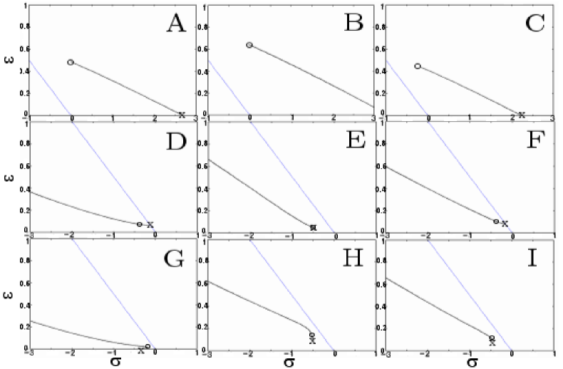
where the truncation is imposed to close the hierarchy at $\ell=10$. For most applications of the flow equations, the exact widths of distributions in (16) are unimportant as long as the hierarchy is convergent. Figure 1 shows $(\sigma,\epsilon)$ trajectories from nine initial configurations. They are all consistent with the linearised analysis in Table II.

Figure 1: Sample of nine $(\sigma,\epsilon)$ trajectories. Circles denote initial random points. Crosses mark where the observable perturbations are produced. In each panel the blue line is the horizontal nullcline (9) Models A,B,C show the most generic behaviour for all values of $\mbox{sgn}(\xi)$ (see Table II). The remaining models all violate slow-roll and observables are calculated by backward integration. According to our classification, models D,E and F are clearly consistent with $\xi>0$, whereas $\xi<0$ for G, H and I.

Figure 2: Illustrations of critical areas in the $(\sigma,\epsilon)$ plane. A random point that starts in a yellow region ends up around $\epsilon=0,\sigma>0$ (class A in text). Pink and cyan mark potentially slow-roll violating points whose observables are produced at $\sigma=-2\epsilon$ (class B) and $\epsilon=0,\sigma<0$ (class C) respectively. Boxes indicate the initial $(\sigma_{0},\epsilon_{0})$ window in equation (16). The coloured areas translate to respective abundance of resulting points from a stochastic experiment as summarised in equation (17). However, this breakdown is sensitive to the parameter $N_{\mbox{critical}}$ (the number of e-folds before inflation is terminated abruptly, see text for a more precise definition). For instance, very large $N_{\mbox{critical}}$ renders the top panel entirely pink.

By producing 125,000 realisations, we observed the following distribution among three classes:

1. Asymptotic flow towards the half-line $\epsilon=0,\sigma>0$ (for $\approx 90\%$ of all trajectories).

2. Slow-roll violation with observable perturbations produced at the power-law line $\sigma=-2\epsilon$ (for $\approx 8\%$ of trajectories).

3. Slow-roll violation with observable perturbations produced at $\epsilon=0,\sigma<0$ (for $\approx 2\%$ of trajectories).

This is in agreement with observations in the numerical investigations of references kin ; lid2 ; p03 . We have a simple explanation for this distribution.

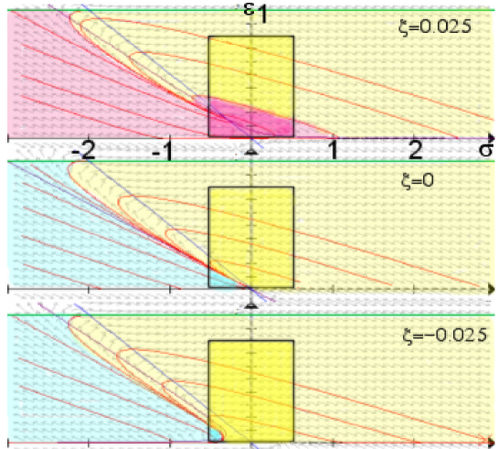
Figure 2 shows the sketches of Table II with the initial window (16) in the $(\sigma,\epsilon)$ plane superimposed, and regions colour-coded according to the eventual fate (A, B or C above) of points starting within them. One deduces that the ratio of these colour-coded areas determines the final distribution in a given stochastic experiment. Formally, for the uniform distributions of equation (16) we have :

Percentage of points in class X

$$\approx\sum_{\mbox{sgn}(\xi)}\frac{\mbox{area for outcome X}}{\mbox{area of }(\sigma_{0},\epsilon_{0})\mbox{ window}}\phantom{t}.\phantom{t}\phantom{t}\phantom{t}\phantom{t}$$ (17)

where $X=$ A, B or C described above. The sum can be evaluated for $\xi=0,\pm\langle|\xi_{0}|\rangle\approx 0,\pm\max({\xi})/2$. Applying (17) to our case where $\pm\langle|\xi_{0}|\rangle=\pm 0.025$, one easily deduces from Figure 2, for example, that the dominant yellow area in the three panels corresponds to the majority of points belonging to class (A), whereas the tiny cyan areas mean that models belonging to class (C) are very rare indeed.

Figure 2 also shows the effect of changing the size and location of window $(\sigma_{0},\epsilon_{0})$ in (16). For instance, if $\max(\epsilon_{0})<0.8$, the percentage of points in case (A) will drop proportionally. The fraction of trajectories in each of the classes (A), (B) and (C) depends primarily on the initial distributions of the parameters $\sigma$ and $\epsilon$, rather than the initial distributions of higher-order parameters.

Finally, we comment on a particular aspect of numerical solutions of the flow equations. Consider the case when $\xi_{0}>0$. From Table II, one expects all trajectories to violate slow-roll. In particular, a trajectory may appear to approach the line $\epsilon=0,\sigma>0$, but eventually it inevitably intersects the vertical nullcline (10) and swiftly reverses direction, thereafter violating slow-roll. In practice, however, one identifies a flow to be asymptotic (and obeying slow-roll) if it supports inflation until a prescribed critical number of e-folds is fulfilled. In our code, this number is set to $N_{\mbox{\scriptsize{critical}}}=200$. Therefore, trajectories that could eventually violate slow-roll for $N>N_{\mbox{\scriptsize{critical}}}$ are not identified as such in practice. This explains why in Figure 2 there are points that will not violate slow-roll even though $\xi>0$. Of course, to select only truly asymptotic flows, one may increase $N_{\mbox{\scriptsize{critical}}}$ to be, say, 1000 or more. However, this is at the expense of proportionally increased computation time.

To summarise, the numerical implementation of the flow equations described here agrees with theoretical analysis of the flow dynamics, based on the parameter $\xi$, described in the previous Section. There is some dependence of the numerical solutions on input parameters such as the e-fold cut-off $N_{\mbox{\scriptsize{critical}}}$ and choice of initial $(\sigma,\epsilon)$ window (with weak sensitivity to distributions of higher order flow variables). These dependences can be understood theoretically. In particular, we interpreted the distribution of numerical outcomes as ratio of areas in the theoretical phase-space.

III Structures in the space of observables

At about 55 e-folds before the end of inflation, observable perturbations were produced, setting the values of key inflationary observables- for example, the scalar spectral index $n_{s}$ , tensor-scalar ratio $r$ and running of spectral index $\frac{dn_{s}}{d\ln k}$. To second order, these are related to the inflationary flow variables by lpb :

$$r \simeq 16\epsilon[1-C(\sigma+2\epsilon)]\phantom{t},$$ (18)

$$n_{s} \simeq 1+\sigma-(5-3C)\epsilon^{2}-{1\over 4}(3-5C)\sigma\epsilon+{1\over 2}(3-C)\xi\phantom{t},$$

$${dn_{s}\over d\ln k} = -{1\over 1-\epsilon}\cdot{dn_{s}\over dN}\phantom{t},$$ (20)

where $C=0.0814514$. Note that kin ; lid2 define $r$ to be 16 times smaller than in equation (18).

We can now make the following classification:

• If inflation ends by violation of slow-roll conditions, then according to our earlier analysis, observable perturbations were produced either at (i) the line $\epsilon=-2\sigma$, or (ii) $\epsilon=0,\sigma<0$. In the first case, we have an exact power-law inflation, in which case the relation

  $$n_{s}\simeq 1-{2r\over 16-r}\phantom{t},$$ (21)

  holds kin . For case (ii), one observes

  $$r\simeq 0\quad,\quad n_{s}\lesssim 1\phantom{t}.$$ (22)

• If inflation does not violate slow-roll but ends abruptly, then we must have asymptotic flow along $\epsilon=0,\sigma>0$. This yields a ‘blue’ spectrum :

  $$r\simeq 0\quad,\quad n_{s}\gtrsim 1\phantom{t}.$$ (23)

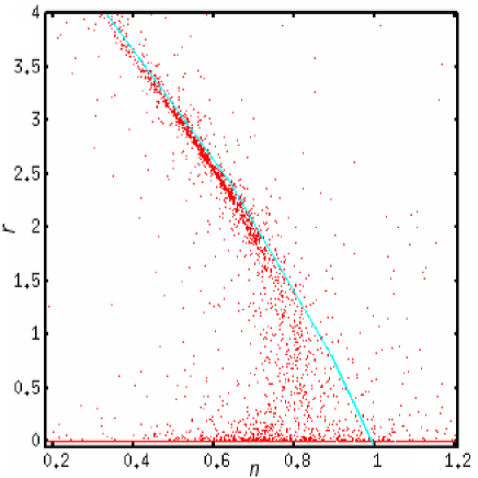
Equations (21), (22) and (23) define three prominent structures in the $(n_{s},r)$ plane where we expect points to cluster strongly. From the analysis of the previous section, we also know the relative density of these structures: Most points cluster at (23) (class A) , some at the power-law curve (21) (class B), and very few at (22) (class C). This behaviour is seen clearly in Figure 3, which shows a scatter plot from $125,000$ numerical solutions of the flow equations using the code and initial conditions described in the previous section.

Figure 3: Models in the $(n_{s},r)$ plane generated from the flow equations. The line $r=0$ is densely populated. The swathe of points traces the curve given by (21) (shown by the blue line). The distribution of points along this line is discussed in text.

In terms of the parameter $\xi$, we deduce that the swathe corresponding to equation (21) is made up almost entirely of models in which $\xi(55)>0$. The $r=0$ cluster should theoretically be made up of only those models with $\xi(55)\leq 0$, although in practice, the choice of $N_{\mbox{\scriptsize{critical}}}$ means that there are some points with $\xi(55)>0$ on this line as well.

Figure 4: Numerical simulations similar to those shown in Figure 3, but for different values of $N_{\mbox{\scriptsize{obs}}}$. As $N_{\mbox{\scriptsize{obs}}}$ increases, the swathe of points around equation (21) moves to lower values of $r$ as described in the text.

The swathe is not evenly populated along the curve (21). We have a simple explanation for this non-uniformity. Starting at the end of inflation with $\xi(0)>0$ and $\epsilon(0)=1$, the trajectory is traced 55 e-folds backward in time, at which point the trajectory must be near the line $\sigma=-2\epsilon$ in order to form the swathe in the $(n_{s},r)$ plane. From Table I, the $\epsilon$ coordinate of the power-law fixed point is

$$\epsilon_{*}=\sqrt{\xi}<1\phantom{t}.$$

From (18), to first order,

$$r\simeq 16\epsilon(55)\geq 16\epsilon_{*}=16\sqrt{\xi(55)}\phantom{t},$$

so that :

$$16\sqrt{\xi(55)}\phantom{t}\lesssim\phantom{t}r<16\phantom{t},$$ (24)

where $\xi(55)$ is given by equation (15). Only points within these bounds are expected to lie close to the line defined by equation (21). Intuitively, we should expect to see some sharp features in the swathe because trajectories that give rise to the swathe are suddenly terminated 55 e-fold by backward integration in order to calculate $r$. For example, in Figure 3, the lower bound in (24) is found to be 1.7 on average. For $r\lesssim 1.7$, the points show a large scatter in the $(n_{s},r)$ plane and no longer cluster tightly around the relation defined by equation (21).

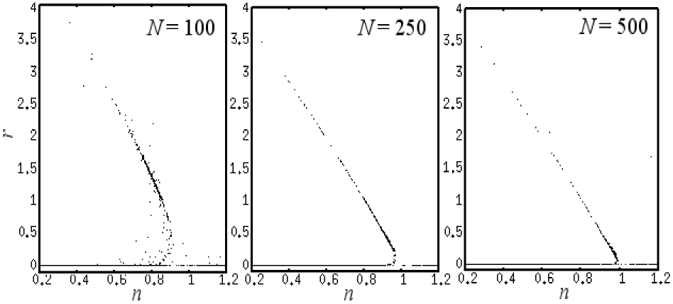
Finally, we comment on the sensitivity of the swathe to the e-fold limit $N_{\mbox{\scriptsize{obs}}}=55$ when observable perturbations are generated. As discussed earlier, the investigations of leach ; dod favour a range of $N_{\mbox{\scriptsize{obs}}}$ between 50 to $60$, but caution that some models with prolonged reheating may give $N_{\mbox{\scriptsize{obs}}}$ as high as 100. We investigate how such an increase affects the structures in the $(n_{s},r)$ plane.

An increase in $N_{\mbox{\scriptsize{obs}}}$ only affects slow-roll violating models. In the case where observable perturbations are produced along the line $\epsilon=0,\sigma<0$, extended backward integration gives rise to a larger spread along the line $n_{s}<1$ in the observable plane. On the other hand, for those trajectories approaching the power-law line $\sigma=-2\epsilon$, an increase in $N_{\mbox{\scriptsize{obs}}}$ means that $\xi$ exponentially decays towards zero for a longer time, concentrating the points to lower values of $r$. Furthermore, as $N_{\mbox{\scriptsize{obs}}}$ is increased, the analogous lower bound to (24) extends to lower values of $r$. Thus for large values of $N_{\mbox{\scriptsize{obs}}}$, points cluster tightly around equation (21) to values of $r$ close to zero. These effects are evident in Figure 4, which shows analogous plots to Figure 3, but for numerical simulations with $N_{\mbox{\scriptsize{obs}}}$ is the range $100$ to $500$.

IV Physical interpretations

In the slow-roll approximation, the potential shape is parametrized by its slope and curvature via the slow-roll parameters :

$$\epsilon_{V}={m_{\mbox{\scriptsize{Pl}}}^{2}\over 16\pi}\Big{(}{V^{\prime}\over V}\Big{)}^{2}\quad,\quad\eta_{V}={m_{\mbox{\scriptsize{Pl}}}^{2}\over 8\pi}\Big{(}{V^{\prime\prime}\over V}\Big{)}\phantom{t}.$$ (25)

We wish to see precisely how the flow parameters $\{\epsilon,\sigma,^{\ell}\lambda_{H}\}$ relate to this description of the potential shape.

As stated in the introduction, the flow parameters are related to $V(\phi)$ via the Hamilton-Jacobi equation (4). Dividing it by $H^{2}$ gives a useful form :

$$\epsilon-3=-{8\pi\over m_{\mbox{\scriptsize{Pl}}}^{2}}\Big{(}{V\over H^{2}}\Big{)}\phantom{t}.$$ (26)

By differentiating (4), we can derive two further relations:

$$\pm\sqrt{\epsilon}(\eta-3)=-2{\sqrt{\pi}\over m_{\mbox{\scriptsize{Pl}}}}\Big{(}{V^{\prime}\over H^{2}}\Big{)}\phantom{t},$$ (27)

$$\eta^{2}-3(\epsilon+\eta)+\xi=-{V^{\prime\prime}\over H^{2}}\phantom{t},$$ (28)

where the sign of $\sqrt{\epsilon}$ matches that of $H^{\prime}$. Equations (26) to (28) relate the amplitude, gradient, and curvature (in that order) of the potential $V$ to the flow parameters.

Now consider the first slow-roll condition $\epsilon_{V}\ll 1$. This condition states that the slope of the potential should be so small that (i) potential energy dominates kinetic energy of the field ($V\gg\dot{\phi}^{2}$) and (ii) rolling approaches ‘terminal’ speed so that $\ddot{\phi}\approx 0$. By dividing (27) by (26) we obtain these requirements exactly in terms of flow parameters:

$$\epsilon_{V}=\epsilon\Big{(}{\eta-3\over\epsilon-3}\Big{)}^{2}\ll 1\phantom{t}.$$ (29)

One way to maintain inflation is to ensure that the potential becomes increasingly flat, so that the inflaton continues approaching the minimum asymptotically. From (29), this can be achieved with a small $\epsilon$ regardless of how large $|\eta|$ is. In the $(\sigma,\epsilon)$ phase-space, this corresponds to those ‘hybrid’ type trajectories approaching $\epsilon=0$ regardless of large $\sigma$.

Next, the second slow-roll condition $|\eta_{V}|\ll 1$ can be obtained by differentiating $\epsilon_{V}$, and so it places a restriction on the potential curvature. By dividing (28) by (26), we can recast this condition as

$$|\eta_{V}|=\bigg{|}{3(\epsilon+\eta)-{\eta^{2}}-\xi\over 3-\epsilon}\bigg{|}\ll 1\phantom{t}.$$ (30)

(Note the role of parameter $\xi$ as a constraint on the curvature.) In particular, we see that a universe with sufficiently large negative $\eta$ will violate (30) even though the first slow-roll condition (29) is satisfied. This shows why potentials with sufficiently large negative curvature (such as those associated with spontaneous symmetry breaking or new inflation as ; linde ) are doomed to violate slow-roll. As the inflaton gains speed along a concave-down potential, its ‘image’ in the phase-space is a flow towards the line $\{\epsilon=1,\sigma\leq-2\}$ as shown in Table II.

In summary, one can understand the correspondence between inflaton motion along a potential and the flow in $\{\epsilon,\sigma,^{\ell}\lambda_{H}\}$ phase-space simply by using the flow parameters to characterize the gradient and curvature of the potential.

V conclusions

The inflationary flow equations have been used by a large number of authors to draw inferences about observable parameters. When solving the flow equations, one finds favoured regions of observable parameters due to dynamical attractors. The purpose of this paper has been to examine the dynamics of the flow equations analytically. In particular, we have shown that the Hubble ‘jerk’ parameter $\xi$ effectively discriminates the stability of fixed points in the flow parameter phase-space, while the dynamics of $\xi$ itself can be described simply in terms of exponential decay. Using this technique, we were able to explain complicated motions in the $\{\epsilon,\sigma,^{\ell}\lambda_{H}\}$ phase-space analytically. The distribution of points and stability of structures in the plane of observables can also be understood in terms of dynamics of $\xi$. Comparing our analytic work with numerical solutions of the flow equation, we found that they were in good agreement. Finally, we have given exact relations showing how the trajectories in the phase-space of flow variables correspond physically to motion of the inflaton along a potential.

The main features in the plane of observables are generally insensitive to the initial configuration (i.e. choice of values ${}^{\ell}\lambda_{H}\big{|}_{0}$) - although there is a dependence on the parameter $N_{\mbox{\scriptsize{critical}}}$ which can be understood dynamically. Thus we believe that we understand the main features of the solutions of the flow equations. Nevertheless, to interpret diagrams such as figures 3 and 4 in any statistical sense requires an understanding of the thorny issue of measures and how initial conditions for inflation might translate into distributions of initial configurations. We have not attempted to address these problems in this paper. For some speculations, see references vil ; tegmark .

Acknowledgements: SC acknowledges the Dorothy Hodgkin scholarship from PPARC. This work has been supported by grants from PPARC.

References

- (1) Lyth D.H. and Riotto A., Phys.Rept. 314, 1 (1999)
- (2) Quevedo F., Class.Quant.Grav. 19, 5721 (2002)
- (3) Hoffman M.B. and Turner M.S., Phys. Rev. D64, 023506 (2001)
- (4) Kinney W.H., Phys. Rev. D66, 083508 (2002)
- (5) Liddle A.R. and Lyth D.H., ‘Cosmological Inflation and Large-Scale Structure’, CUP (2000)
- (6) Liddle A.R., Phys. Rev. D68, 103504 (2003)
- (7) Easther R. and Kinney W.H., Phys. Rev. D67, 043511 (2003)
- (8) Liddle A.R. and Leach S.M., Phys. Rev. D68, 103503 (2003)
- (9) Dodelson S. and Hui L., Phys. Rev. Lett. 91, 131301 (2003)
- (10) Ramirez E. and Liddle A.R., Phys. Rev. D71, 123510 (2005)
- (11) Peiris H.V., et al. Ap.J. Suppl., 148, 213 (2003)
- (12) Efstathiou G., Mack K.J., JCAP 0505 008 (2005)
- (13) Liddle A.R., Parsons P. and Barrow J.D., Phys. Rev. D50, 7222 (1994)
- (14) Albrecht A. and Steinhardt, P.J., Phys. Rev. Lett. 48, 1220 (1982)
- (15) Linde A.D., Phys. Lett., B108, 389 (1982)
- (16) Garriga J. and Vilenkin A., Phys. Rev. D64, 023507, (2001)
- (17) Tegmark M., JCAP 0504 001 (2005)