Reduced Shear Power Spectrum

Abstract

Measurements of ellipticities of background galaxies are sensitive to the reduced shear, the cosmic shear divided by $(1-\kappa)$ where $\kappa$ is the projected density field. We compute the difference between shear and reduced shear both analytically and with simulations. The difference becomes more important on smaller scales, and will impact cosmological parameter estimation from upcoming experiments. A simple recipe is presented to carry out the required correction.

I Introduction

One of the most fascinating aspects of general relativity, and the first triumph for the theory, is that gravitational potentials can act as lenses for light from distant sources. The presence of large-scale structure and its associated potentials along the line-of-sight to distant galaxies implies that the images of most distant galaxies are slightly sheared compared to their intrinsic shapes. This shearing effect encodes information about cosmological distances and the evolution of large-scale structure. For this reason gravitational lensing of background galaxies by large scale structure (cosmic shear) offers an excellent way to study the distribution of matter in the universe Kaiser (1992); Mellier (1999); Bartelmann and Schneider (2001); Dodelson (2003). Measurements of the cosmic shear are already enabling us to constrain the dark matter abundance and clustering amplitude among other parameters Hoekstra et al. (2002); Van Waerbeke et al. (2004); Heymans et al. (2004); Jarvis et al. (2005). In the future, large surveys may well uncover properties of dark energy, such as its abundance and equation of state Benabed and Bernardeau (2001); Refregier et al. (2004); Takada and Jain (2004); Heavens (2003), and of neutrinos Hu and Tegmark (1999); Abazajian and Dodelson (2003). This program will be successful only if we can make very accurate theoretical predictions Huterer and Takada (2004).

As experiments begin to go deeper and cover more and more sky, theorists must make sure that predictions are accurate enough to extract cosmological information in an unbiased fashion. There is a quantitative way to phrase this directive: the systematic errors on cosmological parameters induced by theoretical uncertainties should be significantly smaller than the anticipated statistical errors. Since the latter hover near the percent level for the most ambitious experiments, theorists clearly have their work cut out for them.

Here we consider one correction to the standard theoretical predictions, the effect of reduced shear Schneider et al. (1998); Barber (2002); White (2005). The observed ellipticities of galaxies (with two components $g_{i}$ for each galaxy) are often used as estimates of the cosmic shear ($\gamma_{i}$), but in fact they are sensitive to the reduced shear:

$$g_{i}={\gamma_{i}\over 1-\kappa},\quad\left|\kappa\right|<1$$ (1)

where $\kappa$ is the convergence or roughly the projected density field. We analyze the difference between shear and reduced shear both analytically and with numerical simulations Vale and White (2003); White and Vale (2004), focusing on various two-point functions. Then we map out the region in experiment-space where the effects of reduced shear need to be included. Outside of this region, the canonical prediction – which neglects the $1-\kappa$ denominator – is sufficient.

Throughout we assume a flat, $\Lambda$CDM cosmology. Our base model has $\Omega_{m}=0.28$, $\Omega_{b}h^{2}=0.024$, $h=0.7$, $n=1$, and $\sigma_{8}=0.9$. We will let the galaxy density and sky coverage of surveys vary, but we limit ourselves to all background sources at $z=1$. Our quantitative results will change slightly for higher redshift sources, but our two major conclusions – that we can compute these corrections accurately and that we have to compute them if we want to extract cosmological parameters – are only strengthened (since the effect is larger) for higher redshift sources.

II Shear Two-Point Functions

Here we briefly review a variety of definitions relating to cosmic shear and its statistics. Cosmic shear can be represented by two numbers at any point in space, $\gamma_{1}$ and $\gamma_{2}$. Similarly, the ellipticity of a background galaxy can be described by $g_{1}$ and $g_{2}$. The latter are measurable, while the former are related in a straighforward way to the projected gravitational potential and therefore are simplest to compute given a cosmological theory. On average, all these components are zero; however their two-point functions contain information about cosmic fluctuations.

We focus here on four sets of two-point functions.

• Smoothed Variance Defining $\gamma\equiv\gamma_{1}+i\gamma_{2}$, make a map of $\gamma$ smoothed over a square pixel of side $\theta$. The variance of the smoothed shear field, $\bar{\gamma}$, is then

  $$\langle|\bar{\gamma}^{2}|\rangle(\theta)=\langle\bar{\gamma}_{1}^{2}\rangle(\theta)+\langle\bar{\gamma}_{2}^{2}\rangle(\theta)$$ (2)

  with a similar definition for the galaxy ellipticities, $g$. Note that “$\bar{\quad}$” denotes an average over a local square while angle brackets denote an average over the sky.

• Aperture Mass At any sky position $\theta_{0}$, this is a 2D integral over the tangential shear, $\gamma_{t}\equiv-\gamma_{1}\cos(2\phi)-\gamma_{2}\sin(2\phi)$, where $\phi$ is the angle between $\theta_{0}$ and a fixed $x$-axis. The weighting function in the integral depends on a smoothing scale $\theta$. Here we use the smoothing function defined in Schneider et al. (1998). The average value of $M_{\rm ap}$ is zero, but its variance as a function of smoothing scale contains information about the underlying fluctuations.

• Correlation Function Since there are two components of shear, there are in principle 3 separate correlation functions $\langle\gamma_{i}($$\theta_{0}$$)\gamma_{j}($$\theta_{0}$$+$$\theta$$)\rangle$ averaged over all positions $\theta_{0}$. These depend on the angular difference $\theta\equiv|$$\theta$$|$. Here we focus on the combination $\xi(\theta)\equiv\langle\gamma($$\theta_{0}$$)\gamma^{*}($$\theta_{0}$$+$$\theta$$)\rangle$.

• Angular Power Spectrum Write the $\gamma_{i}$ field as a sum of coefficients times spherical harmonics. In the small angle limit in which we will work, this is equivalent to a Fourier transform, $\tilde{\gamma}_{i}({\bf l})$. One linear combination of these Fourier coefficients (the so-called “B-mode”) vanishes if the underlying fluctuations are due to scalar perturbations; the other,

  $$\tilde{E}({\bf l})=\epsilon_{ij}T_{i}({\bf l})\tilde{\gamma}_{j}({\bf l}),$$ (3)

  is sensitive to the projected gravitational potential. Here $\epsilon_{ij}$ is the 2D anti-symmetric tensor $\epsilon_{12}=-\epsilon_{21}=1$; and the trigonometric weighting functions are

  $$T_{1}({\bf l}) \equiv -\sin(2\phi_{l})$$

  $$T_{2}({\bf l}) \equiv \cos(2\phi_{l})$$ (4)

  where $\phi_{l}$ is the angle of ${\bf l}$ with a fixed $x$-axis. The angular power spectrum is roughly the variance of these Fourier coefficents,

  $$\langle\tilde{E}({\bf l})\tilde{E}({\bf l}^{\prime})\rangle=(2\pi)^{2}\delta^{2}\left({\bf l}+{\bf l}^{\prime}\right)C_{l}.$$ (5)

Each of these two-point functions can be computed from a simulation using either shear or reduced shear. Thus, for example, we can measure in a simulation both $C_{l}^{\gamma}$ and $C_{l}^{g}$ and find the difference between the two. The simulations we use to compute these functions are described in Ref. White (2005). We can also compute the two-point functions semi-analytically. The two-point functions of $\gamma$ can be expressed in terms of integrals over the 3D matter power spectrum, which has been extremely well-studied Hamilton et al. (1991); Peacock and Dodds (1994, 1996); Bernardeau et al. (2002); Smith et al. (2003). The two-point functions of $g$ can be computed perturbatively by expanding the $1-\kappa$ denominator around $\kappa=0$. In §III, we write the shear two-point functions as integrals of the 3D matter power spectrum (these expressions are well-known Kaiser (1992); Dodelson (2003)) and the reduced shear corrections in terms of the 3D three-point function, the matter bispectrum.

III Perturbative Calculation

The simplest two point function to compute is the angular power spectrum. The Fourier transformed shear can be expressed in terms of the projected gravitational potential

$$\tilde{\gamma}_{i}({\bf l})=-\epsilon_{ij}T_{j}({\bf l}){l^{2}\over 2}\tilde{\psi}({\bf l})$$ (6)

with

$$\tilde{\psi}({\bf l})\equiv\int_{0}^{\infty}{d\chi\over\chi}W(\chi)\int{dk_{3}\over 2\pi}\tilde{\Phi}({\bf l}/\chi,k_{3};\chi).$$ (7)

Here $\chi$ is comoving distance; the lensing kernel $W=2\chi(1-\chi/\chi_{s})\Theta(\chi_{s}-\chi)$ with $\chi_{s}$ the distance to the source galaxy and $\Theta$ the Heaviside step function.

Inserting Eq. (6) into Eq. (3) to get $\tilde{E}({\bf l})$, multiplying $\tilde{E}({\bf l})$ by $\tilde{E}({\bf l}^{\prime})$, taking the expectation value, and then integrating over ${\bf l}^{\prime}$ in the Limber approximation leads to

$$C_{l}={l^{4}\over 4}\int{d\chi W^{2}(\chi)\over\chi^{6}}P_{\Phi}(l/\chi;\chi)$$ (8)

where $P_{\Phi}$ is the 3D power spectrum of the gravitational potential. The top panel of Fig. 1 shows the power spectrum computed in this fashion as compared with that measured in simulations. Agreement is excellent, confirming earlier work Jain et al. (2000); Hu and White (2001). The one aberrant point on small scales in the simulations is close to the Nyquist frequency, so power in the simulation is artifically suppressed.

Figure 1: Results from simulations (points with error bars) and the perturbative calculation (smooth curves) for the zero order power spectrum (top panel) and the fractional change due to reduced shear (bottom panel).

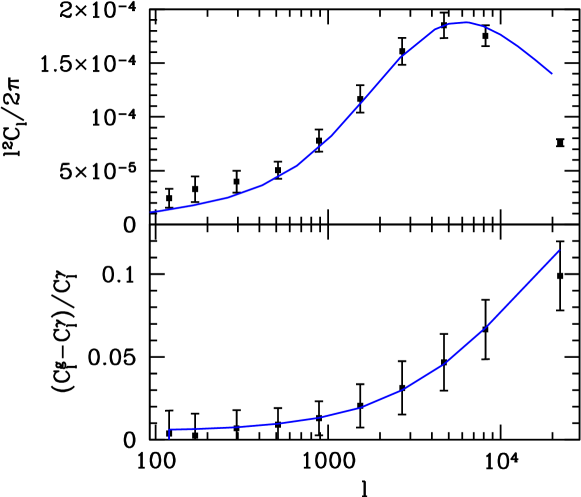
Eq. (8) is an expression for the power spectrum of cosmic shear, $C_{l}^{\gamma}$. To lowest order, when $\kappa\rightarrow 0$ in Eq. (1), the power spectrum of the observable reduced shear is equal to this. We can perturbatively compute the correction to the reduced shear: to leading order, $g^{(1)}=\gamma$ and to second order $g^{(2)}=\gamma\kappa$. Therefore, the correction to the two-point function due to reduced shear is

$$\delta\langle\tilde{E}({\bf l})\tilde{E}({\bf l}^{\prime})\rangle=\epsilon_{ij}\epsilon_{kl}T_{i}({\bf l})T_{k}({\bf l}^{\prime})\langle\tilde{g}_{j}^{(2)}({\bf l})\tilde{g}_{l}^{(1)}({\bf l}^{\prime})\rangle+\left({\bf l}\leftrightarrow{\bf l}^{\prime}\right)$$ (9)

Plugging in for $\tilde{E}$ and using $\epsilon_{ij}\epsilon_{jk}=-\delta_{ik}$, we have

$$\delta\langle\tilde{E}({\bf l})\tilde{E}({\bf l}^{\prime})\rangle={-l^{2}\over 8}T_{i}({\bf l})\int{d^{2}l_{1}\over(2\pi)^{2}}T_{i}({\bf l}_{1})l_{1}^{2}({\bf l}-{\bf l}_{1})^{2}\langle\tilde{\psi}({\bf l}_{1})\tilde{\psi}({\bf l}-{\bf l}_{1})\tilde{\psi}({\bf l}^{\prime})\rangle+\left({\bf l}\leftrightarrow{\bf l}^{\prime}\right)$$ (10)

Using Eqs. (19,20) and (22) in Ref. Dodelson and Zhang (2005), we can reduce this to

$$\delta C_{l}={2T_{i}(l)\over l^{4}}\int{d^{2}l_{1}\over(2\pi)^{2}}T_{i}({\bf l}_{1})l_{1}^{2}({\bf l}-{\bf l}_{1})^{2}B^{\kappa}({\bf l}_{1},{\bf l}-{\bf l}_{1},-{\bf l})$$ (11)

where $B^{\kappa}$ is the bispectrum of the convergence. Just as the power spectrum of the convergence can be written as an integral of the 3D power spectrum along the line-of-sight (Eq. (8)), the 2D bispectrum is an integral of the 3D bispectrum Castro (2003):

$$B^{\kappa}({\bf l}_{1},{\bf l}_{2},{\bf l}_{3})={-l^{6}\over 8}\int_{0}^{\infty}d\chi{W^{3}(\chi)\over\chi^{10}}B_{\Phi}({\bf l}_{1}/\chi,{\bf l}_{2}/\chi,{\bf l}_{3}/\chi).$$ (12)

The 3D bispectrum, $B_{\Phi}$, has been computed analytically on large scales and measured on a wide range of scales in simulations Bernardeau et al. (2002). An accurate fit to the N-body results was introduced in Ref. Scoccimarro and Couchman (2001); we use this fit to compute $\delta C_{l}$, the difference between cosmic shear and reduced shear power. The power spectrum, $P_{\Phi}$, which is needed to compute $B_{\Phi}$, was computed using the publicly available Halofit code Smith et al. (2003) which has also been calibrated by numerical simulations. Fig. 1 shows the results of this perturbative calculation and of a similar measurement from simulations. The perturbative results are in excellent agreement with the simulations. This is extremely encouraging because it offers an easy way to include reduced shear corrections without resorting to expensive simulations.

The conclusion that reduced shear differs from cosmic shear most significantly on small scales follows from perturbation theory. On large scales, fluctuations in $\gamma$ and $\kappa$ are small; since the difference between cosmic shear and reduced shear is higher order in these perturbations $(\propto\kappa\gamma)$, it is very small on large scales.

The angular two-point functions described in §II can all be expressed as integrals over the power spectrum. The smoothed variance is

$$\langle|\bar{\gamma}^{2}|\rangle(\theta)={1\over\pi^{2}}\int d^{2}l\tilde{j}_{0}(l_{1}\theta/2)j_{0}(l_{2}\theta/2)C_{l}.$$ (13)

This variance can be computed for either shear or reduced shear. The difference between the two is the same integral over $\delta C_{l}$ from Eq. (11). The other spatial functions are

$$\langle M_{\rm ap}^{2}\rangle(\theta)={288\over\pi\theta^{4}}\int_{0}^{\infty}dl{C_{l}J_{4}^{2}(l\theta)\over l^{3}}$$ (14)

and

$$\xi(\theta)={1\over 2\pi}\int_{0}^{\infty}dllJ_{0}(l\theta)C_{l}.$$ (15)

Figure 2: Angular two-point functions from simulations and perturbatively.

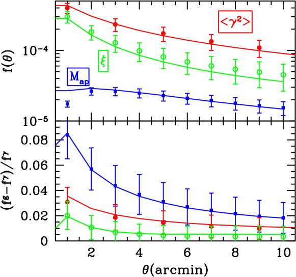
We have computed these three functions from simulations and perturbatively; the results are shown in Fig. 2. The simulations and perturbative calculations agree extremely well, as do the corrections.

IV Impact on Cosmological Parameters

When does one need to include the effects of reduced shear when comparing models with observations? Neglecting these effects results in an incorrect prediction for the power spectrum; we computed a correction, $\delta C_{l}$, above. This incorrect prediction propagates to an incorrect estimate of the cosmological parameters, $p_{i}$, or a bias. The bias on parameter $i$ is

$$b_{i}\equiv p_{i}^{\rm true}-p_{i}=F^{-1}_{ij}\sum_{l}w_{l}{\partial C_{l}\over\partial p_{j}}\delta C_{l}.$$ (16)

Here $w_{l}$ is the weight, the inverse variance of the measurement, and $F$ is the Fisher matrix

$$F_{ij}=\sum_{l}w_{l}{\partial C_{l}\over\partial p_{i}}{\partial C_{l}\over\partial p_{j}}.$$ (17)

The variance depends on experimental specifications: sky coverage and depth/resolution. Specifically,

$$w_{l}^{-1}={2\over(2l+1)f_{\rm sky}}\left(C_{l}+{\langle\gamma_{\rm int}^{2}\rangle\over n_{\rm eff}}\right).$$ (18)

The fraction of sky covered is $f_{\rm sky}$, while the rms of the intrinsic ellipticity of galaxies, $\langle\gamma_{\rm int}^{2}\rangle^{1/2}$, is set to $0.25$ Hoekstra et al. (1999); Refregier et al. (2004), and $n_{\rm eff}$ is the effective galaxy density which depends mainly on the depth and resolution of the experiment.

We can compute the bias induced by neglecting the difference between shear and cosmic shear for any experiment. For concreteness, we allow three cosmological parameters to vary: the normalization of the power spectrum, $\sigma_{8}$; the shape of the power spectrum, $\Gamma\simeq\Omega_{m}h$; and the matter density, $\Omega_{m}$. Figure 3 shows the bias induced in these parameters by neglected the cosmic shear corrections. This bias was computed including data out to $l=3000$. The cut-off is necessary because baryons affect the theoretical predictions on small scales White (2004); Zhan and Knox (2004), and it is very difficult to predict these effects accurately.

Figure 3: The bias due to neglecting reduced shear corrections as a function of galaxy density (per square arcminute for a 1-component rms shear of $0.25$) for the three cosmological parameters varied. The bias on $\sigma_{8}$ is negative.

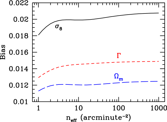
Since the reduced shear corrections on scales $l<3000$ are of order a few percent (Fig. 1), it is not surprising that the induced biases on the parameters are also of order a few percent. Note from Eq. (16) that the bias scales as $F^{-1}w_{l}$. Since $w_{l}\propto f_{\rm sky}^{-1}$, and $F^{-1}$ scales as $f_{\rm sky}$ the bias is nearly independent of sky coverage. Therefore, the bias depends only on the galaxy density. At very large density, the weight $w_{l}$ becomes independent of galaxy density, since shape noise due to intrinsic ellipticity is inversely proportional to galaxy density. In this limit, cosmic variance – the first term in parentheses in Eq. (18) – becomes the dominant source of noise. The largest bias is to the normalization parameter $\sigma_{8}$.

How important is a one to two percent level bias in the cosmological parameters? We must compare the bias to the anticipated statistical error in an experiment. If there were only one free parameter, this comparison would be straightforward. With several parameters, we must ask which statistical error should be used as a baseline: the error on $\sigma_{8}$ for example which accounts for the uncertainty in all other parameters (this is called the marginalized error) or the error expected if all other parameters are held fixed? We argue that the latter should be used. To understand why, consider the case with two parameters. The expected 1-$\sigma$ constraints trace out an ellipse in this plane. If the parameters are degenerate, this ellipse is very elongated, and the expected constraints on either of the parameters individually will be very weak. If these marginalized errors are used, then the ratio (bias/error) will be quite small. A bias much smaller than the marginalized statistical error, however, can easily induce an analyst to estimate the parameter as lying outside the allowed ellipse. If we instead use unmarginalized errors as the baseline, then bias/statistical error ratios smaller than one are more likely to keep the parameters within the allowed ellipse. Fig. 4 shows the ensuing ratio of bias to statistical error for the most severely affected cosmological parameter ($\sigma_{8}$) as a function of survey width ($f_{\rm sky}$) and galaxy density.

Figure 4: The ratio of the bias on $\sigma_{8}$ due to neglecting reduced shear to the statistical error on $\sigma_{8}$. The ratio depends on the width and galaxy density of the survey. Several current and future surveys are shown for orientiation: CTIO Lensing Survey Jarvis et al. (2005); Supernova Acceleration Probe (SNAP) Albert et al. (2005); Dark Energy Survey (DES) [http://www.darkenergysurvey.org]; Large Scale Synaptic Survey (LSST) Tyson et al. (2003). If the ratio is larger than one, neglecting reduced shear corrections biases the parameters by an amount greater than the unmarginalized statistical errors.

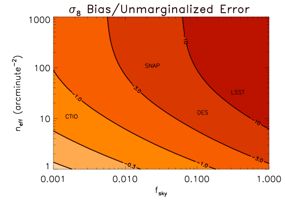
Alternatively, we can transform to a basis in parameter space where the Fisher matrix is diagonal and then rescale so that the errors on the parameters are unity. In this basis, magnitude of the bias is a simple measure of how far outside (or inside) the 1-sigma contours the bias leads. Again a bias greater than unity means the effect needs to be accounted for. Figure 5 shows the bias in this rotated/rescaled basis. For example, neglecting the bias in the dark energy survey leads to an incorrect estimate of parameters at the 3-sigma level.

Figure 5: The bias for rotated and rescaled parameters such that the anticipated errors are diagonal and unity. That is, the 1-sigma contours in the 3D parameter space map out a sphere of radius one in this basis. The amplitude of the bias is shown here as a function of galaxy density and sky coverage.

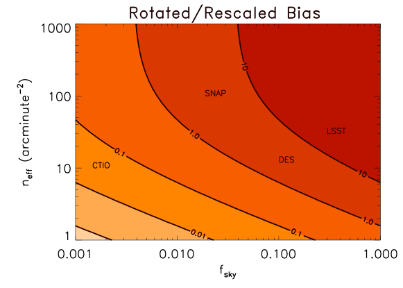
Both Figures 4 and 5 illustrate that the largest of current experiments are already entering a regime in which the effects of reduced shear must be considered and future experiments will certainly need to account for it. Relying on Fig. 5 to justify neglecting the effect for current experiments is a little dangerous since it does not account for priors, which can reduce errors while leaving the bias unaffected. So the most conservative approach is to use Fig. 4 as a guide to the impact of reduced shear. In that case, virtually all upcoming experiments will need to add in this correction when extracting information about cosmological parameters.

V Other Corrections

Reducing the shear is not the only correction that needs to be applied to weak lensing spectra Jain et al. (2000); Schneider et al. (1998); Vale and White (2003). For instance, Hu and Cooray Cooray and Hu (2002) have computed perturbative corrections to the power spectrum which account for the Born approximation and lens-lens coupling. These corrections are an order of magnitude smaller than the one considered here. To understand why, recall that $\delta C_{l}$ from Eq. (9) comes from considering the product of a second order perturbation with a first order perturbation, $g^{(1)}\times g^{(2)}$. We have considered the corresponding terms for the beyond Born and lens-lens corrections and found that they vanish. Therefore, the first non-vanishing corrections are the ones considered in Ref. Cooray and Hu (2002): those of order $g^{(1)}g^{(3)}$ or $g^{(2)}g^{(2)}$. We have also not considered the effects of source clustering Bernardeau (1998). There is some indication Hamana (2001); Schneider et al. (2002) that this may also induce percent level changes in the power spectrum on small scales. If so, these would need to be included as well. Accounting for this coupling in a simulation requires input from a real 3D galaxy catalogue.

VI Conclusions

Deflection of light rays by gravitational potentials along the line of sight introduces a mapping between the source and image plane. The Jacobian of this mapping defines the shear and convergence as a function of position on the sky. In the absence of size or magnification information neither the shear nor the convergence is observable, but only the combination $g=\gamma/(1-\kappa)$, known as the reduced shear. On small scales, where lensing surveys get much of their constraining power, this must be taken into account when predicting the observables.

We have studied the difference between cosmic shear and the reduced shear. Our main conlusions are:

• The perturbative calculation of reduced shear, Eq. (11), agrees well with numerical simulations. This is not too surprising, since the lensing is weak and we use many components themselves fit to N-body simulations, but it gives us confidence that we can use these calculations in making predictions or fitting to data.

• The effects of reduced shear are on the threshhold of becoming very relevant. As depicted in Figs. 4 and 5, upcoming surveys will need to account for reduced shear when extracting cosmological parameters.

SD was supported by the DOE and by NASA grant NAG5-10842. MJW was supported in part by NASA and the NSF. CAS was supported in part by the Kavli Institute for Cosmological Physics at the University of Chicago and by grant NSF PHY-011442. The simulations were performed on the IBM-SP at NERSC.

References

- Kaiser (1992) N. Kaiser, Astrophys. J. 388, 272 (1992).
- Mellier (1999) Y. Mellier, Ann. Rev. Astron. Astrophys. 37, 127 (1999), eprint astro-ph/9812172.
- Bartelmann and Schneider (2001) M. Bartelmann and P. Schneider, Phys. Rept. 340, 291 (2001), eprint astro-ph/9912508.
- Dodelson (2003) S. Dodelson, Modern Cosmology (Academic Press, San Diego, 2003).
- Hoekstra et al. (2002) H. Hoekstra, H. Yee, and M. Gladders, New Astron. Rev. 46, 767 (2002), eprint astro-ph/0205205.
- Van Waerbeke et al. (2004) L. Van Waerbeke, Y. Mellier, and H. Hoekstra (2004), eprint astro-ph/0406468.
- Heymans et al. (2004) C. Heymans et al. (2004), eprint astro-ph/0411324.
- Jarvis et al. (2005) M. Jarvis, B. Jain, G. Bernstein, and D. Dolney (2005), eprint astro-ph/0502243.
- Benabed and Bernardeau (2001) K. Benabed and F. Bernardeau, Phys. Rev. D64, 083501 (2001), eprint astro-ph/0104371.
- Refregier et al. (2004) A. Refregier et al., Astron. J. 127, 3102 (2004), eprint astro-ph/0304419.
- Takada and Jain (2004) M. Takada and B. Jain, Mon. Not. Roy. Astron. Soc. 348, 897 (2004), eprint astro-ph/0310125.
- Heavens (2003) A. Heavens, Mon. Not. Roy. Astron. Soc. 343, 1327 (2003), eprint astro-ph/0304151.
- Hu and Tegmark (1999) W. Hu and M. Tegmark, Astrophys. J. 514, L65 (1999), eprint astro-ph/9811168.
- Abazajian and Dodelson (2003) K. N. Abazajian and S. Dodelson, Phys. Rev. Lett. 91, 041301 (2003), eprint astro-ph/0212216.
- Huterer and Takada (2004) D. Huterer and M. Takada (2004), eprint astro-ph/0412142.
- Schneider et al. (1998) P. Schneider, L. van Waerbeke, B. Jain, and G. Kruse, Mon. Not. Roy. Astron. Soc. 296, 873 (1998), eprint astro-ph/9708143.
- Barber (2002) A. J. Barber, Mon. Not. Roy. Astron. Soc. 335, 909 (2002), eprint astro-ph/0108273.
- White (2005) M. White, Astropart. Phys. 23, 349 (2005), eprint astro-ph/0502003.
- Vale and White (2003) C. Vale and M. J. White, Astrophys. J. 592, 699 (2003), eprint astro-ph/0303555.
- White and Vale (2004) M. J. White and C. Vale, Astropart. Phys. 22, 19 (2004), eprint astro-ph/0312133.
- Hamilton et al. (1991) A. J. S. Hamilton, A. Matthews, P. Kumar, and E. Lu, Astrophys. J. 374, L1 (1991).
- Peacock and Dodds (1994) J. A. Peacock and S. J. Dodds, Mon. Not. Roy. Astron. Soc. 267, 1020 (1994), eprint astro-ph/9311057.
- Peacock and Dodds (1996) J. A. Peacock and S. J. Dodds, Mon. Not. Roy. Astron. Soc. 280, L19 (1996), eprint astro-ph/9603031.
- Bernardeau et al. (2002) F. Bernardeau, S. Colombi, E. Gaztanaga, and R. Scoccimarro, Phys. Rept. 367, 1 (2002), eprint astro-ph/0112551.
- Smith et al. (2003) R. E. Smith et al. (The Virgo Consortium), Mon. Not. Roy. Astron. Soc. 341, 1311 (2003), eprint astro-ph/0207664.
- Jain et al. (2000) B. Jain, U. Seljak, and S. D. M. White, Astrophys. J. 530, 547 (2000), eprint astro-ph/9901191.
- Hu and White (2001) W. Hu and M. J. White, Astrophys. J. 554, 67 (2001), eprint astro-ph/0010352.
- Dodelson and Zhang (2005) S. Dodelson and P. Zhang (2005), eprint astro-ph/0501063.
- Castro (2003) P. G. Castro, Phys. Rev. D67, 123001 (2003), eprint astro-ph/0212500.
- Scoccimarro and Couchman (2001) R. Scoccimarro and H. M. P. Couchman, Mon. Not. Roy. Astron. Soc. 325, 1312 (2001), eprint astro-ph/0009427.
- Hoekstra et al. (1999) H. Hoekstra, M. Franx, and K. Kuijken (1999), eprint astro-ph/9910487.
- White (2004) M. White, Astropart. Phys. 22, 211 (2004), eprint astro-ph/0405593.
- Zhan and Knox (2004) H. Zhan and L. Knox (2004), eprint astro-ph/0409198.
- Albert et al. (2005) J. Albert et al. (SNAP) (2005), eprint astro-ph/0507460.
- Tyson et al. (2003) J. A. Tyson, D. M. Wittman, J. F. Hennawi, and D. N. Spergel, Nucl. Phys. Proc. Suppl. 124, 21 (2003), eprint astro-ph/0209632.
- Cooray and Hu (2002) A. Cooray and W. Hu, Astrophys. J. 574, 19 (2002), eprint astro-ph/0202411.
- Bernardeau (1998) F. Bernardeau, Astron. Astrophys. 338, 375 (1998), eprint astro-ph/9712115.
- Hamana (2001) T. Hamana, Mon. Not. Roy. Astron. Soc. 326, 326 (2001), eprint astro-ph/0104244.
- Schneider et al. (2002) P. Schneider, L. van Waerbeke, and Y. Mellier, Astron. & Astrophys. 389, 729 (2002).