Structure and scaling of the entropy in nearby galaxy clusters

Using XMM-Newton observations, we investigate the scaling and structural properties of the ICM entropy in a sample of 10 nearby ($z<0.2$) relaxed galaxy clusters in the temperature range 2-9 keV. We derive the local entropy-temperature ($S$–$T$) relation at $R=0.1,0.2,0.3$ and $0.5R_{200}$. The logarithmic slope of the relation is the same within the $1\sigma$ error at all scaled radii. However, the intrinsic dispersion about the best fitting relation is significantly higher at $0.1R_{200}$. The slope is $0.64\pm 0.11$ at $0.3\,R_{200}$, in excellent agreement with previous work. We also investigate the entropy-mass relation at density contrasts $\delta=5000,2500$ and 1000. We find a shallower slope than that expected in simple self-similar models, which is in agreement with the observed empirically-determined entropy-temperature and mass-temperature scaling. The dispersion is smaller than for the $S$–$T$ relation. Once scaled appropriately, the entropy profiles appear similar beyond $\sim 0.1R_{200}$, with an intrinsic dispersion of $\sim 15$ per cent and a shape consistent with gravitational heating ($S(r)\lower 3.0pt\hbox{$\,\buildrel\textstyle\propto\over{\textstyle\sim}\,$}r^{1.1}$). However, the scatter in scaled entropy profiles increases with smaller scaled radius, to more than $60$ per cent at $R\lesssim 0.05R_{200}$. Our results are in qualitative agreement with models which boost entropy production at the accretion shock. However, localised entropy modification may be needed to explain the dispersion in the inner regions.

1 Introduction

X-ray observations of the hot, gaseous intracluster medium (ICM) have been telling us for well over a decade that physical processes other than gravity are acting to modify the properties of the cluster population. An understanding of the source(s) of this modification is of great importance for our understanding of cluster formation and evolution, and is essential for the use of clusters as precision cosmological probes.

Entropy is important because, together with the shape of the potential well, it is the quantity which dictates the observed X-ray properties of the ICM in galaxy clusters (Voit, 2005). The intracluster entropy is generated in shocks as gas is drawn into the gravitational potential of the cluster halo (Tozzi & Norman, 2001; Borgani et al., 2001; Voit et al., 2002, 2003; Voit, 2005; Borgani et al., 2005), thus it reflects the accretion history of the ICM. However, the entropy distribution also preserves key information regarding the influence of non-gravitational processes.

X-ray measurements of the entropy at $0.1R_{200}$ (hereafter $S_{0.1}$) showed that the entropy of the coolest systems is considerably higher than that available from gravitational collapse (Ponman et al., 1999; Lloyd-Davies et al., 2000), and that the entropy-temperature ($S$–$T$) relation is shallower than expected (Ponman et al., 2003). More recent spatially resolved entropy profiles indicate that the entropy is higher throughout the ICM, and that, outside the core regions, entropy profiles are structurally similar (Ponman et al., 2003; Voit & Ponman, 2003; Pratt & Arnaud, 2003, 2005; Piffareti et al., 2005). At the same time the scatter in $S_{0.1}$ at a given temperature can be up to a factor of three (Ponman et al., 2003).

Possible entropy modification mechanisms have historically included preheating, where the gas has been heated before being accreted into the potential well, by early supernovae and/or AGN activity (e.g., Kaiser, 1991; Evrard & Henry, 1991; Valageas & Silk, 1999), internal heating after accretion (e.g., Metzler & Evrard, 1994), and cooling (e.g., Pearce et al., 2000). The lack of isentropic core entropy profiles in groups and poor clusters has shown that simple preheating is unlikely to be the sole explanation of the observations (Ponman et al., 2003; Pratt & Arnaud, 2003, 2005). Since cooling-only models generally predict a higher stellar mass fraction than observed (e.g., Muanwong et al., 2002), attention is now focussing on the interplay between cooling and feedback. Further high quality observations are needed in order to distinguish between these different entropy modification mechanisms.

Figure 1: Cluster entropy profiles obtained from the deprojected, PSF corrected temperature profiles and the best fitting analytical model for the gas density. Solid lines, included to improve visibility, are entropy profiles obtained from analytic model fits to the temperature and density information. On the left, the profiles are plotted in physical units ($h_{70}^{-1}$ kpc); on the right, they are plotted in units of $R_{200}$.

The present paper is the third in a series based on XMM-Newton observations of ten clusters in the temperature range from 2 keV to 9 keV. In Pointecouteau, Arnaud & Pratt (2005, hereafter Paper I), we investigated the shape and scaling properties of the dark matter distribution, and in Arnaud, Pointecouteau & Pratt (2005, hereafter Paper II) we examined the relation between the total mass and the X-ray temperature. In the present paper we extend the work of Pratt & Arnaud (2005) by exploring the entropy scaling properties over a larger temperature/mass range.

All results given below were calculated assuming a $\Lambda$CDM cosmology with $\Omega_{m}=0.3$ and $\Omega_{\Lambda}=0.7$ and $H_{0}=70$ km s^-1 Mpc^-1. Unless otherwise stated, errors are given at the $68$ per cent confidence level.

2 Sample and analysis

Table 1: Basic cluster data.

Cluster	z	T
		(keV)
A1983	0.0442	$2.18\pm 0.09$
A2717	0.0498	$2.56\pm 0.06$
MKW9	0.0382	$2.43\pm 0.24$
A1991	0.0586	$2.71\pm 0.07$
A2597	0.0852	$3.67\pm 0.09$
A1068	0.1375	$4.67\pm 0.11$
A1413	0.1427	$6.62\pm 0.14$
A478	0.0881	$7.05\pm 0.12$
PKS0745	0.1028	$7.97\pm 0.28$
A2204	0.1523	$8.26\pm 0.22$

The sample (Table 1) comprises 10 systems ranging in temperature from 2 keV to $\sim 8.5$ keV. In Paper I, spatially resolved temperature and density data were used to calculate gravitating mass profiles. These were which then fitted with an NFW model, yielding values for $M_{\rm 200}$ and $R_{200}$ (’virial’ mass and radius corresponding to a density contrast of 200). The mean temperature of each system, $T_{\rm spec}$, needed to investigate the scaling properties of the profiles, was estimated from fits to a spectrum built from all events in the region $0.1R_{200}\,\leq r\leq\,0.5R_{200}$ (see the discussion in Paper II). The data reduction steps are described in detail in Paper I.

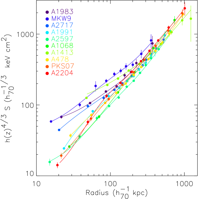
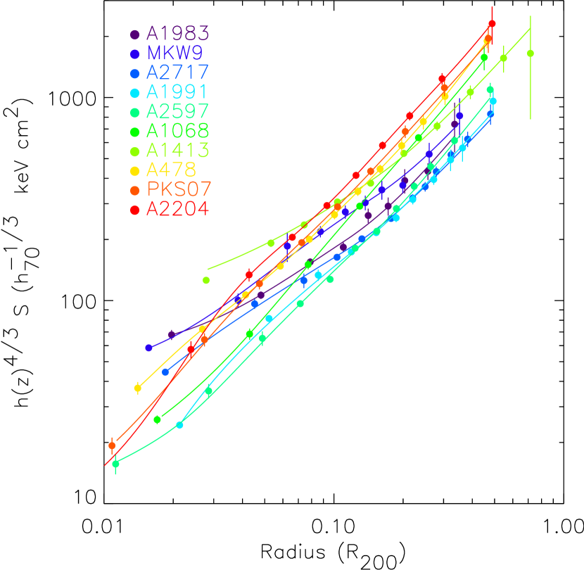
We calculated the entropy profile of each system using the deprojected, PSF corrected temperature profile and an analytical model for the gas density derived in Paper I. Analytic gas density model parameters are listed in Appendix A. In Fig 1, the raw entropy profiles are shown in physical units ($\rm h_{70}^{-1}$ kpc), and in terms of the measured virial radius, $R_{200}$. All profiles increase monotonically with radius and, while the slope of the profile becomes shallower towards the centre in some of the clusters, none shows an isentropic core.

3 Entropy scaling properties

3.1 Introduction

In a self-similar cluster population expected from simple gravitational collapse, the scaled profiles of any physical quantity coincide, and thus measures of these quantities at any scaled radius should correlate with global quantities such as the mean temperature, or the virial mass. In this standard model, the entropy is expected to scale as $S\propto h(z)^{-4/3}T$ or $S\propto h(z)^{-2/3}M^{2/3}$.

In purely theoretical terms, the most fundamental characteristic of a cluster is its mass. Previous investigations of the entropy scaling relations were hampered in this respect because they did not have accurate mass information. The present observations, which have excellent mass data (Papers I and II), thus represent an ideal opportunity to examine the entropy-mass relation. In addition, the spatial resolution and radial coverage in the entropy profiles are significantly improved, as compared with previous ROSAT/ASCA studies (Ponman et al., 2003). In this Section, we investigate both the entropy-temperature ($h(z)^{4/3}S$–$T_{\rm spec}$) and the entropy-mass ($h(z)^{2/3}S$–$M_{\rm 200}$) relations. We derive the slope and normalisation of each relation, at various scaled radius/density contrasts. We also estimate the raw, statistical and intrinsic scatter about the relations.

Table 2: The $S$–$T$ relation. Data were fitted with a power-law of the form $h(z)^{4/3}\leavevmode\nobreak\ S=A\times({\rm k}T/{\rm 5keV})^{\alpha}$, where ${\rm k}T$ is the overall spectroscopic temperature in the $0.1-0.5\leavevmode\nobreak\ R_{200}$ region. Errors in entropy and temperature are taken into account. Results are given for the WLS, BCES, and WLSS regression methods (see text). Raw, statistical and intrinsic scatter about the best fitting relation in the log-log plane are given in the last columns; the numbers in parentheses indicate the percentage intrinsic scatter.

Radius	$A$	$\alpha$	$\sigma_{log}$
$R_{200}$	keV cm-2		raw	stat	int
WLS
0.1	$227\pm 5$	$0.58\pm 0.05$	0.079	0.030	0.073
0.2	$478\pm 12$	$0.73\pm 0.06$	0.058	0.035	0.047
0.3	$770\pm 24$	$0.71\pm 0.07$	0.074	0.043	0.060
0.5	$1510\pm 90$	$0.68\pm 0.12$	0.070	0.078	-
BCES
0.1	$230\pm 17$	$0.49\pm 0.15$	0.082	0.030	0.076 $\scriptstyle(19\%)$
0.2	$485\pm 22$	$0.62\pm 0.11$	0.063	0.034	0.052 $\scriptstyle(13\%)$
0.3	$798\pm 44$	$0.64\pm 0.11$	0.078	0.043	0.065 $\scriptstyle(16\%)$
0.5	$1560\pm 83$	$0.62\pm 0.08$	0.074	0.078	-
WLSS
0.1	$229\pm 16$	$0.47\pm 0.14$	0.083	0.030	0.077
0.2	$480\pm 23$	$0.67\pm 0.10$	0.059	0.035	0.048
0.3	$786\pm 43$	$0.69\pm 0.12$	0.075	0.043	0.061
0.5	$1510\pm 90$	$0.68\pm 0.12$	0.070	0.078	-

Figure 2: The $S$-$T$ relation measured from a sample of 10 clusters covering a temperature range from 2 to 9 keV. The $S$-$T$ relation is shown for different fractions of $R_{200}$. Measurements are plotted with error bars. At each radius, the best-fitting power-law relation, derived taking account the errors in entropy and temperature, is overplotted. Solid line: BCES regression method; dashed line: WLS method; slopes and intercepts are given in Table 2.

3.2 Method

The entropy estimates at a given scaled radius ($x=r/R_{200}$) or density contrast ($\delta$) have to be calculated taking into account the uncertainties on the temperature, the analytical gas density model, and the measurement of the scaled radius/density contrast itself. We thus estimated the entropy at a given $x$ or $\delta$, and the associated errors, using a Monte Carlo method. The scaled radius $r(x)$/$R_{\delta}$ values and corresponding uncertainties were estimated from NFW-type modelling of the mass profile (see Papers I and II for details), and subsequently randomised assuming a Gaussian distribution with sigma equal to the $1\sigma$ error. The temperature profile was then similarly randomised taking into account the observed uncertainties, and the temperature estimated at the relevant (randomised) $r(x)$/$R_{\delta}$ using spline interpolation. The entropy was then calculated in the usual manner, $S={\rm k}T/n_{e}^{2/3}$, including an additional $5$ per cent systematic error on $n_{e}$ (corresponding to the uncertainties in the surface brightness profile modelling; see Paper I). This procedure was undertaken 1000 times for each cluster; the final entropy value at each $x$/ $\delta$ was calculated from the mean and standard deviation of the randomised values at that radius.

The temperature profiles of all systems except A1983 and MKW9 are detected up to $\sim 0.5\,R_{200}$ (the scaled radius/density contrast of maximum detection of A1983 and MKW9 are $0.38R_{200}$/1455$\delta$ and $0.41R_{200}/1401\delta$, respectively). The temperature profiles of these clusters had thus to be extrapolated to $0.5R_{200}$/$1000\delta$. To avoid spuriously high/low temperatures, we only allowed extrapolations within $\pm 1.5$ times the mean temperature of the cluster (well within the range of temperature gradients observed to date, e.g., Arnaud et al. 2005; Vikhlinin et al. 2005).

3.3 The $S$–$T$ relation

Our data have the required temperature coverage to investigate the entropy-temperature relation. For easier comparison with previous work, we first investigated the $S$–$T$ relation at different fractions of the virial radius, viz., 0.1, 0.2, 0.3, and $0.5\leavevmode\nobreak\ R_{200}$. We fitted a power law model of the form

$$h(z)^{4/3}\leavevmode\nobreak\ S_{\rm x}=A[T_{\rm spec}/{\rm 5\leavevmode\nobreak\ keV}]^{\alpha}$$ (1)

to the data, $T_{\rm spec}$ being defined as in Sect. 2. We chose a pivot point of 5 keV for consistency with the $M$–$T$ relation of Arnaud et al. (2005). The fit was performed using linear regression in the log-log plane, taking into account the errors on both variables. We have also computed the raw and intrinsic scatter about the best fitting relations in the log-log plane. To estimate the raw scatter, we used the vertical distances to the regression line, weighted by the error. The intrinsic scatter was computed from the quadratic difference between the raw scatter and the scatter expected from the statistical errors. The resulting values are given in Table 2.

In undertaking the fits, we first used the classical weighted least square method, WLS ($\chi^{2}$ estimator) implemented in the the routine FITEXY from numerical recipes (Press et al., 1992). This regression method is strictly valid only if the intrinsic scatter is negligible as compared to the statistical scatter. This is generally not the case (see Table 2). We thus also considered the orthogonal BCES method (Akritas & Bershady, 1996), with bootstrap resampling. This is the least-biased regression method when both measurement errors and intrinsic scatter are present. However, no error weighting is performed on individual data points. We thus also considered a variation of the WLS method, where a constant term, corresponding to the intrinsic scatter, is added quadratically to the $\log(S)$ error (WLSS method). The best fit is determined such that the reduced $\chi^{2}$, after minimization over $A$ and $\alpha$, is $\chi^{2}_{\rm red}=1$.

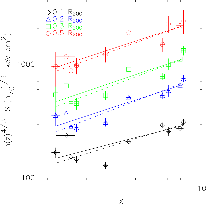
The best fitting slopes and intercepts for the different methods are listed in Table 2. Figure 2 shows the data and the best-fitting power law relation for each radius under consideration, obtained using the standard WLS and BCES methods. The three methods give best fitting parameters consistent within the $1\sigma$ errors. However, the errors are underestimated with the WLS method, especially at low radii. This is a consequence of the high $\chi^{2}$ value obtained, reflecting the high intrinsic scatter at small scaled radius (e.g. $\chi^{2}=54$ for 8 d.o.f at $0.1\leavevmode\nobreak\ R_{200}$). In this case the standard $\Delta\chi^{2}=1$ criteria to derive parameter errors is not valid. The BCES and WLSS give results in excellent agreement with each other, both in terms of best-fitting values and associated uncertainties. In the following, for easier comparison with previous work, we will refer to results obtained using the commonly used BCES method.

The slope of the entropy-temperature relation is incompatible with the standard self-similar prediction at all radii at which we have measured it, confirming the results of Ponman et al. (2003). Our best-fitting $S_{0.1}$–$T$ slope ($\alpha=0.49\pm 0.15$) is slightly shallower than that found by Ponman et al. from unweighted orthogonal regression on individual data points ($\alpha=0.65\pm 0.05$). A better agreement is observed with the slope derived by these authors from data grouped in temperature bins ($\alpha=0.57\pm 0.04$). However, the slopes are consistent once uncertainties are taken into account.

Beyond $r\geq 0.2\,R_{200}$, the slope remains remarkably stable. At $0.3R_{200}$, our gas density and temperature measurements are well constrained, and do not suffer potential systematic problems connected to the correction for PSF and projection effects. At this radius, we are well outside the strong cooling cores found in the majority of the objects in our sample. In addition, we note that there are no significant temperature gradients at this radius in the high resolution temperature profiles produced by Vikhlinin et al. (2005) from Chandra observations. For this reason we consider the measurements at $0.3R_{200}$ to be the most reliable. The slope of the $S_{0.3}$-$T$ relation, obtained using the BCES method, is $S_{0.3}\propto T^{0.64\pm 0.11}$, in excellent agreement with that found by Ponman et al. (2003).

Figure 2 shows that there is noticeable scatter about the $S_{0.1}$–$T$ relation. Table 2 makes clear that the scatter is reduced at larger scaled radius. The intrinsic scatter remains the dominant contributor to the dispersion in all relations, except at $0.5\leavevmode\nobreak\ R_{200}$.

3.4 The $S$–$M$ relation

Table 3: The $S$–$M$ relation. Data were fitted with a power-law model of the form $h(z)^{2/3}\leavevmode\nobreak\ S_{\delta}=B_{\delta}\times(M_{200}/5.3\times 10^{14}M_{\odot})^{\beta}$, where $M_{200}$ is the total mass obtained from NFW model fits to the measured mass profiles. Best-fitting relations are given for the BCES estimator, taking into account errors in mass and entropy. Results are given for the full sample, and for the sample excluding MKW9, which is a significant outlier. The numbers in parenthesis indicate the percentage intrinsic scatter.

$\delta$	$B$	$\beta$	$\sigma_{log}$
	keV cm-2		raw	stat	int
Full
sample
5000	$471\pm 18$	$0.36\pm 0.10$	0.058	0.034	0.046 $\scriptstyle(11\%)$
2500	$765\pm 30$	$0.37\pm 0.10$	0.059	0.041	0.043 $\scriptstyle(10\%)$
1000	$1460\pm 47$	$0.36\pm 0.06$	0.059	0.065	-
Excl.
MKW9
5000	$459\pm 37$	$0.43\pm 0.10$	0.039	0.035	0.017 $\scriptstyle(4\%)$
2500	$741\pm 43$	$0.44\pm 0.08$	0.035	0.041	-
1000	$1430\pm 46$	$0.41\pm 0.04$	0.042	0.063	-

Figure 3: The $S$–$M$ relation measured at various density contrasts. $M_{200}$ values were measured from NFW model fits to the measured mass profiles (Papers I and II). Symbols with error bars represent the measurements. Lines show the best-fitting power-law $S$–$M$ relation: solid: full sample; dashed: excluding MKW9. Slopes and intercepts are given in Table 3.

In investigating the $S$–$M$ relation, it is more logical to work in terms of density contrast $\delta$. We used $\delta=5000$, 2500, and 1000, which correspond to average fractions of $0.20\pm 0.01\leavevmode\nobreak\ R_{200}$, $0.29\pm 0.02\leavevmode\nobreak\ R_{200}$ and $0.47\pm 0.02\leavevmode\nobreak\ R_{200}$ for the present sample, and fitted a power law of the form

$$h(z)^{2/3}S_{\delta}=B_{\delta}[M_{200}/5.3\times 10^{14}M_{\odot}]^{\beta}$$ (2)

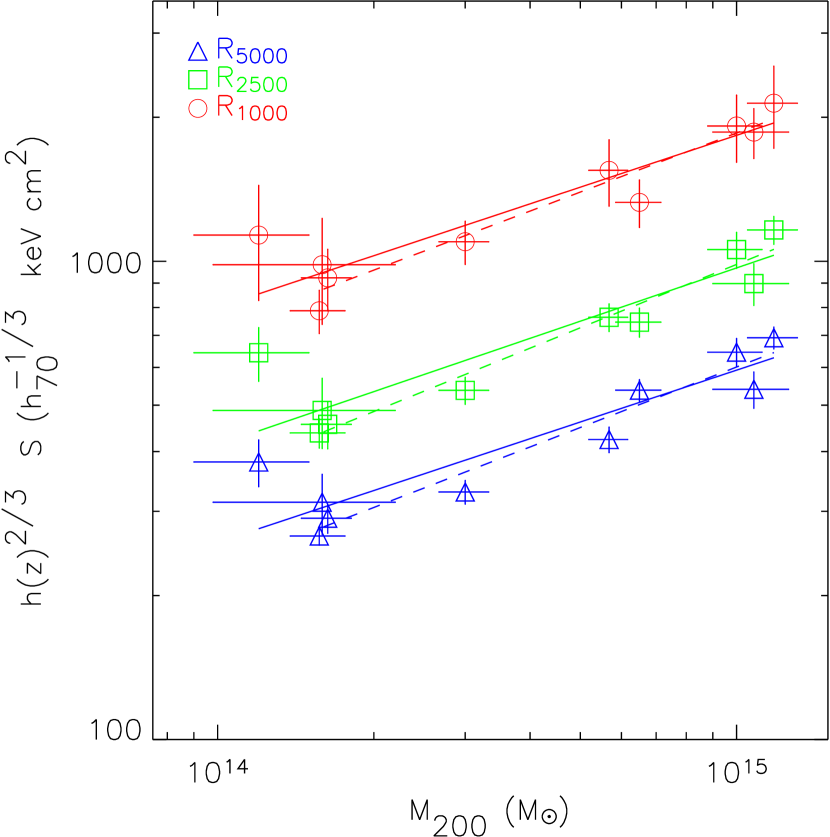
to the data. The pivot point of $5.3\times 10^{14}M_{\odot}$ corresponds to a temperature of 5 keV using the best-fitting $M$–$T$ relation of Arnaud et al. (2005). In Fig 3 we show the data and the best-fitting power law relation for each density contrast under consideration. Since MKW9 appears to be a clear outlier, we also fitted the relation excluding this cluster. The best fitting slopes and intercepts for the $S$–$M$ relation, with and without MKW9, are listed in Table 3.

The best-fitting $S$–$M$ relation is shallower than the prediction from standard self-similar models. The results for the full sample are entirely consistent with the observed $S$–$T$ and $M$–$T$ relations (Sect. 3.3 and Paper II). Excluding MKW9, the slope is slightly, although not significantly, steeper.

As can clearly be seen in Fig. 3, and as quantified in Table 3, the intrinsic dispersion about the $S$–$M$ relations is less than that for the $S$–$T$ relations. This is particularly true for the sample excluding MKW9. This is not an artifact of the larger statistical mass errors compared to those on the temperature: the dispersion is similarly smaller for the raw scatter. Table 3 also indicates that, excluding MKW9, the dispersion is now dominated by the statistical scatter at all density contrasts.

4 Scaled entropy profiles

We have confirmed that the $S$–$T$ relation is shallower than expected in the standard self-similar model, and we have shown that this is also true for the $S$–$M$ relation. In this Section, we examine the structural properties of the entropy profiles. We do this by looking at the entropy profiles once scaled by the best fitting relations.

4.1 Scaled entropy versus $r/R_{200}$

In Fig. 4 we show the profiles scaled using the relation $S\propto h(z)^{-4/3}\,T_{10}^{0.65}$, where $T_{10}$ is the global temperature measured in units of 10 keV. This relation is consistent with our data (Table 2), and allows us to compare our results with previous work. As an initial measure of the scatter in scaled entropy profiles, we estimated the dispersion at various radii in the range $0.02$–$0.45\,R_{200}$. The shaded area in Fig 4 shows the region enclosed by the mean plus/minus the $1\sigma$ standard deviation. Figure 4 shows that, outside the core regions, the entropy profiles present a high degree of self-similarity. The relative dispersion in scaled profiles remains approximately constant at $\lesssim 20$ per cent for $r\gtrsim 0.1\,R_{200}$, in excellent agreement with the dispersion found in a smaller subsample by Pratt & Arnaud (2005). In the core regions, however, the dispersion increases with decreasing radius to reach $\gtrsim 60$ per cent at $\sim 0.02\leavevmode\nobreak\ R_{200}$.

Figure 4: Scaled entropy profiles. The radius is scaled to $R_{200}$ measured from the best-fitting mass models (Papers I and II). The entropy is scaled using the empirical entropy scaling $S\propto h(z)^{-4/3}T_{10}^{0.65}$, using the global temperature, $T$, as listed in Table 1, in units of 10 keV. The shaded grey area corresponds to the region enclosed by the mean plus/minus the $1\sigma$ standard deviation. The dashed line denotes $S\propto R^{1.08}$.

Figure 5: Scaled entropy profiles. The radius is expressed as a function of density contrast, $\delta$. The entropy has been scaled with the best-fitting entropy-mass scaling $S_{2500}\propto h(z)^{-2/3}M_{15}^{0.44}$, using the measured total mass, $M_{200}$, in units of $10^{15}$ M_⊙. The shaded grey area corresponds to the region enclosed by the mean plus/minus the $1\sigma$ standard deviation (including MKW9). The solid line shows the power law relation, $S\propto\delta^{-0.66}$, obtained from fitting points with $\delta<15000$ excluding MKW9. The dashed line is an extrapolation of this best fit.

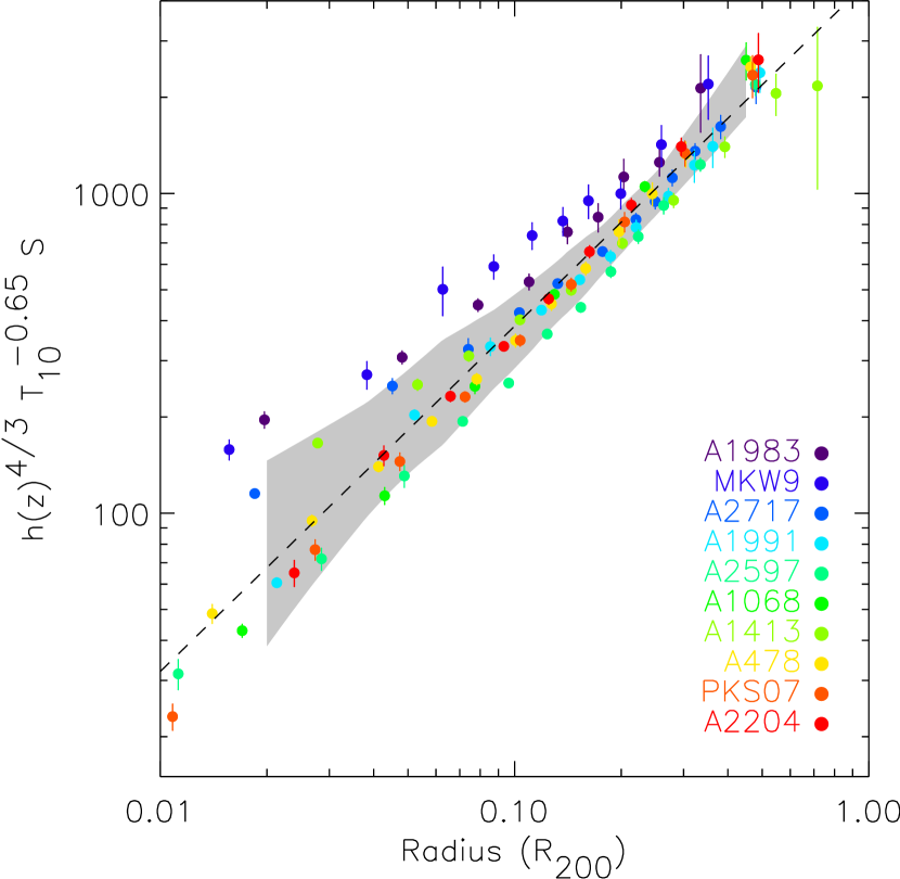
We next fitted the scaled profiles with a power law using the BCES method. The fit was performed in the log-log plane taking into account the errors on both variables. Fitting the data in the radial range $r\geq 0.01\,R_{200}$ we find a slope of $1.08\pm 0.04$, with a dispersion of $\sim 30$ per cent about the best fitting line. The slope is not significantly changed ($1.14\pm 0.06$) if the data are fitted in the radial range $r\geq 0.1\,R_{200}$, but the intrinsic dispersion is two times smaller ($14$ per cent).

For comparison, Pratt & Arnaud (2005), using a subsample of the current data (A1983, MKW9, A2717, A1991 and A1413), found a slope of $0.94\pm 0.14$, while Piffareti et al. (2005), using the same scaling, find a slope of $0.95\pm 0.02$ for their sample of 13 cool core clusters. In contrast, broken power-law behaviour has been found by Mahdavi et al. (2005) for a sample of groups (${\rm k}T\lesssim 2$ keV). Our slightly higher slope, compared to that of Piffareti et al. (2005), can be explained by a slight difference in the temperature profile shape. We note simply that the samples are not equivalent and that a detailed investigation of the slope of the entropy profile will require a carefully controlled, unbiased sample spanning the mass range from groups to massive clusters. Irrespective of the exact slope, that we find $S\lower 3.0pt\hbox{$\,\buildrel\textstyle\propto\over{\textstyle\sim}\,$}r^{1.1}$ is interesting considering that this value is expected for shock heating in spherical collapse (e.g., Tozzi & Norman, 2001). This is further discussed in Sec. 5.

4.2 Scaled entropy versus $\delta$

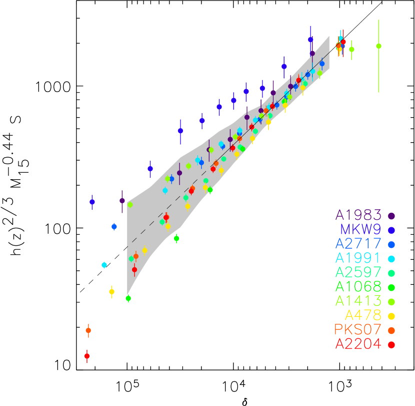
In Figure 5, we show the entropy profiles scaled using the relation $S_{2500}\propto h(z)^{-2/3}\,M_{15}^{0.44}$, where $M_{15}$ is the total mass $M_{200}$ in units of $10^{15}$ M_⊙. Radii are plotted in terms of the density contrast, $\delta$. The shaded area in Fig. 5 shows the region enclosed by the mean plus/minus the $1\leavevmode\nobreak\ \sigma$ standard deviation.

Again, while we observe similarity in the entropy profiles outside the core regions ($\delta\lesssim 15000$), there is a significant increase in the dispersion at higher density contrast. It is also clear that MKW9 is a distinct outlier. This may indicate that the mass of this cluster is underestimated, or its temperature is overestimated. Excluding MKW9 and fitting the scaled entropy profiles with a power law using the BCES method, the slope varies from $-0.76\pm 0.03$ when fitting $\delta<3\times 10^{5}$ ($\sim 0.01\,R_{200}$), to $-0.66\pm 0.03$, when fitting $\delta<15000$ ($\sim 0.1\,R_{200}$). Thus the entropy does not strictly behave as a power-law in density contrast. The intrinsic dispersion drops from $30$ per cent to $10$ per cent depending on the range of density contrast fitted. Outside the core regions, the intrinsic dispersion is smaller than for temperature-scaled profiles, in agreement with the lower dispersion observed for the $S$–$M$ relation compared to that of the $S$–$T$ relation.

5 Discussion

Figure 6: A comparison of our observed entropy profiles with the prediction from the adiabatic numerical simulations of Voit (2005). Left panel: The observed entropy profiles have been scaled to $S_{200}$ using Equation 4. The solid line represents the best-fitting power law relation found by Voit (2005) from fitting adiabatic numerical simulations of 30 clusters in the radial range $0.1<R_{200}<1.0$. Right panel: Ratio between the observed profiles and the best-fitting power law relation found by Voit (2005). The dashed line shows the same relation multiplied by 1.2 to take into account the difference of 30 percent between the observed normalistion of the $M$–$T$ relation and that found in adiabatic simulations.

Our results put into evidence two main departures from the standard self-similar model of cluster formation. First, beyond the core region ($r\gtrsim 0.1\,R_{200}$) the entropy profiles obey self-similarity, having a shape consistent with expectations, but with a modified temperature (or mass) scaling. The scaling relations are shallower than expected. Second, there is a break of similarity in the core region: the dispersion in scaled profiles increases with decreasing radius. In this section, we will discuss in turn both characteristics.

5.1 Entropy normalisation

The modified entropy scaling indicates that there is an excess of entropy, in low mass objects relative to more massive systems, as compared to the expectation from pure shock heating. A comparison with adiabatic numerical simulations allows us to quantify the absolute value of the excess and to examine whether an entropy excess is also present for the most massive systems.

Voit (2005) shows the results of adiabatic numerical simulations of 30 clusters spanning a mass range of more than a factor of ten. Once scaled by the characteristic entropy of the halo,

$$S_{200}=\frac{1}{2}\left[\frac{2\pi}{15}\frac{G^{2}M_{200}}{f_{b}H(z)}\right]^{2/3},$$ (3)

where $f_{b}$ is the baryon fraction, the simulated profiles are closely self-similar, and can be well fitted in the radial range $\sim 0.1-1.0\leavevmode\nobreak\ R_{200}$ by the power-law relation $S/S_{200}=1.26(R/R_{200})^{1.1}$. Assuming $f_{b}=0.14$ ($\Omega_{b}h^{2}=0.02$ and $\Omega_{m}=0.3$) and typical elemental abundances, we can scale our observed entropy values to $S_{200}$ using the expression

$$S/S_{200}=\left(\frac{S}{2471\leavevmode\nobreak\ {\rm keVcm}^{2}}\right)\left(\frac{M_{200}}{1\times 15M_{\odot}}\right)^{-2/3}h(z)^{2/3}.$$ (4)

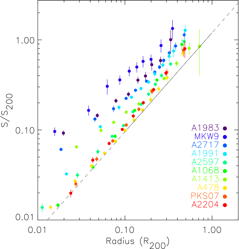
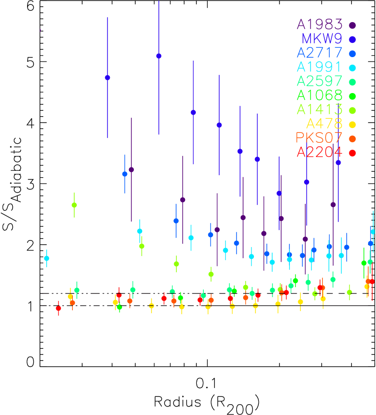
Further scaling the radius by the measured value of $R_{200}$ allows us to compare our results directly with the adiabatic simulations. In the left hand panel of Figure 6, our observed entropy profiles are compared with the prediction of Voit (2005). The right hand panel shows the ratio between the best-fitting adiabatic power-law relation and the observed data.

It can be seen that the richer systems all have entropies which are in good agreement (both in slope and normalisation) with the adiabatic prediction, denoted by the solid line in Fig. 6. On average, their entropy is only slightly higher than predicted (by $\sim 20$ per cent), although the effect is not very significant. We recall that there is also a $\sim 30$ per cent difference in normalisation between the observed $M$–$T$ relation and that predicted by adiabatic simulations (Arnaud et al., 2005). Interestingly, this corresponds to a $\sim 20$ per cent entropy excess at a given mass for $T\propto M^{2/3}$. The (slight) excess of entropy in massive systems is thus consistent with a simple increase of the mean temperature, i.e., of the internal energy of the ICM. However, Fig. 6 shows explicitly that the poorer systems have a systematically higher entropy normalisation than the richer systems. There is approximately 2.5 times more entropy at $0.2\,R_{200}$ in the ICM of A1983, the poorest cluster in our sample, than that predicted by gravitational heating. This excess shows that the density of the ICM is also affected at lower mass.

Voit et al. (2003) and Ponman et al. (2003) independently noted that the ICM entropy is highly sensitive to the density of the incoming gas and suggested that a smoothing of the gas density due to pre-heating in filaments and/or infalling groups would boost the entropy production at the accretion shock. The entropy amplification is more efficient in low mass systems, because they accrete smaller halos more affected by smoothing due to pre-heating. In this interpretation, no substantial isentropic core will develop because the amount of initial preheating needed is substantially less than the characteristic entropy of the final halo. Clusters will thus be self-similar down to low mass but with a modified normalisation scaling as discussed above. This is in agreement with our results outside the core region ($r\gtrsim 0.1R_{200}$).

Recent numerical simulations which mimic preheating by imposing a minimum entropy floor at high $z$ have confirmed the entropy amplification effect due to smooth accretion (Borgani et al., 2005). However, the effect seems to be substantially reduced when cooling is also taken into account. Furthermore, the physical origin of the preheating is still unclear. Heating by SNe seems to be too localised to have a significant effect in smoothing the accreting gas (Borgani et al., 2005). While AGN might be better candidates to produce the extra heating, the observed normalisations require that the AGN affects the entropy distribution at least up to $r_{1000}$. Some recent theoretical investigations suggest that this may be possible (Roychowdhury et al., 2005; Voit & Donahue, 2005).

5.2 Localised modification

While filamentary pre-heating may explain the increased normalisation of poor systems relative to hotter systems, it does not explain the increasing scatter towards the central regions in scaled profiles (Figs. 4,  5 and 6). The adiabatic numerical simulations of Voit (2005) show both a flattening of the slope and an increase in the dispersion of the scaled entropy profiles in the central regions ($<0.1\leavevmode\nobreak\ R_{200}$). However, the dispersion in our observed profiles ($\sim 60$ per cent) greatly exceeds that of the simulations ($\sim 30$ per cent, cf Fig. 6 and Fig. 11 of Voit 2005). Six clusters out of our total sample of ten (A1991, A2597, A1068, A478, PKS0745 and A2204) have remarkably similar scaled entropy profiles, displaying power-law behaviour down to the smallest radii measured. Fitting these scaled profiles in the radial range $0.01-0.1\,R_{200}$ with power-law using the BCES method, we find a slope of $1.13\pm 0.05$, with a dispersion of only 13 per cent. This slope is very similar to that found by fitting the $r>0.1\,R_{200}$ range. These six clusters all appear to host a bona fide cooling core, each having a central temperature decrement of a factor $\sim 2$ (cf Kaastra et al., 2004). Similar power-law profiles were found by in a sample of 13 cooling core clusters by Piffareti et al. (2005). Strong radiative cooling thus appears to generate entropy profiles which display power-law behaviour down to very small radii (Fig. 6). This is similar to the quasi-steady-state entropy profile in the models of McCarthy et al. (2004), which include radiative cooling.

The other four clusters in our sample are characterised by a smaller central temperature decrement, larger cooling times and shallower entropy profiles. Clearly, some mechanism has modified the cooling history of these clusters. Energy input from AGN is regularly invoked as a way of moderating cooling at the centres of galaxy clusters (e.g., Churazov et al., 2001, and references therein). Our sample contains four clusters which have X-ray evidence for interactions between radio and X-ray plasma (A478, A2204, A2597, and PKS0745), and yet the entropy profiles of all of these clusters increase monotonically outward in the canonical fashion. However, we note that Chandra observations of clusters with moderate to strong radio sources (including A478), show some evidence for a slightly shallower slope ($\sim 0.8-0.9$) but only in the very inner regions ($R\lesssim 0.05\leavevmode\nobreak\ R_{200}$; see e.g., Belsole, Birkinshaw & Worrall, 2005; Johnstone et al., 2005; Sanderson, Finoguenov & Mohr, 2004). The effect of AGN activity on the entropy profile will depend on whether the energy input is catastrophic (i.e., occurring in strong bursts) or distributed (more moderated input). It is clear that if the heating is catastrophic in nature, no cluster has yet been found in which this is evident at least from the point of view of the entropy (although see McNamara et al. 2005; Nulsen et al. 2005). The heating is likely more distributed, via e.g., weak shocks (Fabian et al., 2003), thus preserving the generally increasing form of the entropy profile.

Merging events can result in substantial mixing of high and low entropy gas (e.g. Ricker & Sarazin, 2001). Relatively little attention has been given to this possibility in the literature (see, however, Fig. 5 of Voit et al. 2003, Fig. 12 of Belsole et al. 2004 and Fig. 6 of Pratt, Böhringer & Finoguenov 2005). Such redistribution of entropy will depend on the scale of the merger, whether the merger has disrupted the structure of the cool core, and the timescale for re-establishment of the cool core if disrupted. In the current sample MKW9, A2717, A1413 and A1983 all have flatter core entropy profiles. We note that the morphological information for the present sample would argue against recent merger activity in these clusters (Pratt & Arnaud 2005; Papers I and II). However, this does not rule out entropy modification due to a more ancient merger, particularly if the relaxation time is less than the cooling time (see also Belsole et al., 2004).

Table 4: Columns: (1) Cluster name; (2) Parametric model; (3) Central density of principal $\beta$ model ($\times 10^{-2}$ $h_{70}^{1/2}$ cm^-3); (4,5) Central density of second and third $\beta$ model components ($\times 10^{-2}$ $h_{70}^{1/2}$ cm^-3) (6) Core radius of inner $\beta$-model (arcmin); (7) Core radius of principal $\beta$-model (arcmin); (8,9) Core radius of second and third $\beta$ model components (arcmin); (10) $\beta$ parameter; (11) Radius of boundary between $\beta$ model components; (12) $\xi$ parameter; (13) $\chi^{2}$/d.o.f.

Cluster	Model	$n_{e_{1}}$	$n_{e_{2}}$	$n_{e_{3}}$	$r_{c,{\rm in}}$	$r_{c_{1}}$	$r_{c_{2}}$	$r_{c_{3}}$	$\beta$	$r_{\rm cut}$	$\xi$	$\chi^{2}$/d.o.f.
A1983	BB	0.64	–	–	0.49	2.65	–	–	0.76	2.40	1.	71/64
MKW9	BB	0.79	–	–	0.35	3.36	–	–	0.70	3.40	1.	181/133
A2717	BB	1.23	–	-	0.31	1.96	–	–	0.63	2.08	1.	339/206
A1991	BB	5.61	–	-	0.16	1.42	–	–	0.65	2.08	1.	197/160
A2597	KBB	4.30	–	-	0.32	1.21	–	–	0.73	1.92	2.30	158/125
A1068	KBB	40.31	–	-	0.58	3.20	–	–	1.01	4.53	0.25	58/42
A1413	KBB	3.66	–	–	0.41	1.34	–	–	0.71	1.69	0.50	65/47
A478	3B	9.74	2.33	0.36	–	0.25	1.12	3.30	0.84	–	–	50/56
PKS0745	KBB	18.26	–	–	0.19	0.81	–	–	0.64	1.34	0.55	260/214
A2204	3B	15.18	1.42	0.13	–	0.20	1.09	3.87	0.91	–	–	38/44

6 Conclusions

The present sample of ten relaxed clusters constitutes the first with precise mass data and wide temperature coverage, allowing the detailed study of the scaling of ICM entropy with both temperature and mass. The entropy profiles are sampled with good spatial resolution up to $\sim 0.5\,R_{200}$, allowing us to examine structural properties avoiding the stacking analysis and extrapolation on which previous ROSAT/ASCA works relied.

We have found that the entropy profiles of the present cluster sample are self-similar beyond $\sim 0.1\,R_{200}$, with a shape not significantly different from that expected from shock heating. The entropy scaling relations are shallower than expected from standard self-similar models and adiabatic numerical simulations. The slopes of the entropy scaling relations are independent of radius, reflecting the structural self-similarity. The entropy-mass ($S$–$M$) relation is consistent with the observed entropy-temperature ($S$–$T$) and mass-temperature ($M$–$T$) relations. The dispersion is smaller about the $S$–$M$ relation, reflecting the fact that the mass of a cluster is its most fundamental characteristic. These results confirm the trends seen in smaller samples (Pratt & Arnaud, 2005), and in stacking analysis of $\it ROSAT/ASCA$ data (Ponman et al., 2003).

Comparison of our observed profiles with adiabatic numerical simulations has allowed us to quantify the entropy excess relative to that expected in pure gravitational collapse. The excess is only $\sim 20$ per cent in our highest-mass systems. This is in line with a simple increase in the mean temperature consistent with the observed difference in normalisation between the observed $M$–$T$ relation and that predicted by adiabatic simulations. However, the excess in low mass systems can be of more than a factor of 2.5, indicating that the density of the ICM is also affected in these systems. These characteristics are in qualitative agreement with a scenario in which entropy production is boosted at the accretion shock. A plausible candidate mechanism is smoothing of the accreted gas due to preheating (Voit et al., 2003; Ponman et al., 2003).

We have found new and compelling evidence for an increase in the entropy dispersion in the core regions $\sim 60$ per cent at $0.02\,R_{200}$. However the five cooling core clusters in our sample have remarkably self-similar power-law profiles with a dispersion of only 13 per cent between 0.01 and $0.1\,R_{200}$. The observed increase in dispersion towards the central regions argues for localised entropy modification mechanisms. We conclude that AGN activity and/or transient entropy modification due to merging events are good candidates for the modification of cooling in these clusters.

These will be interesting questions to address with numerical simulations. On the observational side, a larger, unbiased, sample of clusters will undoubtedly provide greater insights.

Appendix A Surface brightness profile fit results

The co-added EPIC azimuthally averaged, vignetting corrected, background subtracted surface brightness profile was computed in the [0.3-3.] keV band for each cluster. The profile was corrected for radial variations in the emissivity due to abundance or temperature gradients as described in Pratt & Arnaud (2003). The gas density profile was obtained from fitting parametric analytic models, convolved with the EPIC PSF, to the corrected profile. As discussed in Paper I, we tried various models and empirically chose the best fitting model using the $\chi^{2}$ statistic as a measure of the goodness of fit. The models used were: (i) the double $\beta$ (BB) density model (Pratt & Arnaud, 2002, Eq. 3–5); (ii) the modified double $\beta$ (KBB) model, allowing a more concentrated gas density distribution towards the centre (Pratt & Arnaud, 2002, Eq. 6–8), and (iii) the sum of three $\beta$ (3B) models for the emission measure, in which a common value of $\beta$ is used to ensure smooth behaviour at large radii (Pointecouteau et al., 2004, Eq. 2–3).

The BB and KBB models can be written:

$$\begin{array}[]{lllll}r<r_{\rm cut}&n_{e}(r)&=&n_{e_{1}}&\left[1+\left(\frac{r}{r_{\rm c,in}}\right)^{2\xi}\right]^{-\frac{3\beta_{\rm in}}{2\xi}}\\ r>r_{\rm cut}&n_{e}(r)&=&N&\left[1+\left(\frac{r}{r_{\rm c}}\right)^{2}\right]^{-\frac{3\beta}{2}},\\ \end{array}$$ (5)

where $\xi=1$ for the BB model and $\xi<1$ for the KBB model, and

$$N=n_{e_{1}}\frac{\left[1+\left(\frac{r_{\rm cut}}{r_{\rm c,in}}\right)^{2\xi}\right]^{\frac{-3\beta_{\rm in}}{2\xi}}}{\left[1+\left(\frac{r_{\rm cut}}{r_{\rm c}}\right)^{2}\right]^{-\frac{3\beta}{2}}}$$ (6)

with

$$\beta_{\rm in}=\beta\leavevmode\nobreak\ \frac{1+\left(\frac{r_{\rm c,in}}{r_{\rm cut}}\right)^{2\xi}}{1+\left(\frac{r_{\rm c}}{r_{\rm cut}}\right)^{2}}.$$ (7)

The density profile of the BBB model can be written:

$$n_{e}(r)=\sqrt{n_{e_{1}}^{2}(r)+n_{e_{2}}^{2}(r)+n_{e_{3}}^{2}(r)},$$ (8)

with

$$n_{e_{i}}(r)=n_{e_{i}}\left[1+\left(\frac{r}{r_{c_{i}}}\right)^{2}\right]^{-\frac{3\beta}{2}}.$$ (9)

The best-fitting models, and model parameters, are listed in Table 4.

References

- Akritas & Bershady (1996) Akritas M.G. & Bershady M.A 1996, ApJ, 470, 706
- Arnaud et al. (2005) Arnaud, M., Pointecouteau, E., Pratt, G.W., 2005, A&A, in press (Paper II; astro-ph/0502210)
- Belsole et al. (2004) Belsole, E., Pratt, G.W., Sauvageot, J.-L., Bourdin, H., 2004, A&A, 415, 821
- Belsole et al. (2005) Belsole, E., Birkinshaw, M., Worrall, D.M., 2005, MNRAS, 358, 120
- Borgani et al. (2001) Borgani, S., Governato, F., Wadsley, J., Menci, N., Tozzi, P., Lake, G., Quinn, T., Stadel, J., 2001, ApJ, 559, L71
- Borgani et al. (2005) Borgani, S., Finoguenov, A., Kay, S.T., Ponman, T.J., Springel, V., Tozzi, P., Voit, G.M., 2005, MNRAS, in press (astro-ph/0504265)
- Churazov et al. (2001) Churazov, E., Brüggen, M., Kaiser, C.R., Böhringer, H., Forman, W.R., 2001, ApJ, 554, 261
- Evrard & Henry (1991) Evrard A.E., Henry J.P, 1991, ApJ, 383, 95
- Fabian et al. (2003) Fabian, A.C., Sanders, J.S., Allen, S.W., Crawford, C.S., Iwasawa, K., Johnstone, R.M., Schmidt, R.W., Taylor, G.B., 2003, MNRAS, 344, L43
- Johnstone et al. (2005) Johnstone, R.M., Fabian, A.C., Morris, R.G., Taylor, G.B., 2005, MNRAS, 356, 237
- Kaastra et al. (2004) Kaastra, J., Tamura, T., Peterson, J.R., et al., 2004, A&A, 413, 415
- Kaiser (1991) Kaiser, N. 1991, ApJ, 383, 104
- Kay (2004) Kay, S.T., 2004, MNRAS, 347, L13
- Lloyd-Davies et al. (2000) Lloyd-Davies E.J., Ponman, T.J., Cannon, D.B., 2000, MNRAS, 315, 689
- Mahdavi et al. (2005) Mahdavi, A., Finoguenov, A. B öhringer, H., Geller, M.J., Henry, J.P., 2005, ApJ, 622, 187
- McCarthy et al. (2004) McCarthy, I.G., Balogh, M.L., Babul, A., Poole, G.B., Horner, D.J., 2004, ApJ, 613, 811
- McNamara et al. (2005) McNamara, B.R., Nulsen, P.E.J., Wise, M.W., Rafferty, D.A., Carilli, C., Sarazin, C.L., Blanton, E.L., 2005, Nature, 433, 45
- Metzler & Evrard (1994) Metzler, C.A., Evrard, A.E., 1994, ApJ, 437, 564
- Muanwong et al. (2002) Muanwong, O., Thomas, P.A., Kay, S.T., & Pearce, F.R. 2002, MNRAS, 336, 527
- Nulsen et al. (2005) Nulsen, P.E.J., McNamara, B.R., Wise, M.W., David, L.P., ApJ, in press (astro-ph/0408315)
- Piffareti et al. (2005) Piffaretti, R., Jetzer, P., Kaastra, J.S., Tamura, T., 2005, A&A, 433, 101
- Pearce et al. (2000) Pearce, F.R., Thomas, P.A., Couchman, H.M.P., Edge, A.C., 2000, MNRAS, 317, 1029
- Pointecouteau et al. (2004) Pointecouteau, E., Arnaud, M., Kaastra, J., de Plaa, J., 2004, A&A, 423, 33
- Pointecouteau et al. (2005) Pointecouteau, E., Arnaud, M., Pratt, G.W., 2005, A&A, 435, 1 (Paper I)
- Ponman et al. (1999) Ponman, T.J., Cannon, D.B., Navarro, J.F., 1999, Nature, 397, 135
- Ponman et al. (2003) Ponman, T.J., Sanderson, A.J.R., Finoguenov, A., 2003, MNRAS, 343, 331
- Pratt & Arnaud (2002) Pratt, G.W. & Arnaud, M., 2002, A&A, 394, 375
- Pratt & Arnaud (2003) Pratt, G.W., Arnaud, M., 2003, A&A, 408, 1
- Pratt & Arnaud (2005) Pratt, G.W., Arnaud, M., 2005, A&A, 429, 791
- Pratt et al. (2005) Pratt, G.W., Böhringer, H., Finoguenov, A., 2005, A&A, 433, 777
- Press et al. (1992) Press, W.H., Teukolsky, S.A., Vetterling, S.A. & Flannery B.P., 1992, Numerical Recipes in Fortran 77, Second Edition, p.660
- Ricker & Sarazin (2001) Ricker, P.M., Sarazin, C.L., 2001, ApJ, 561, 621
- Roychowdhury et al. (2005) Roychowdhury, S., Ruszkowski, M & Nath, B.B. 2005, ApJ, in press (astro-ph/0508120)
- Sanderson et al. (2004) Sanderson, A.J.R., Finoguenov, A., Mohr, J.J., 2004, ApJ, submitted (astro-ph/0412316)
- Tozzi & Norman (2001) Tozzi, P., & Norman, C., 2001, ApJ, 546, 63
- Valageas & Silk (1999) Valageas, P., & Silk, J. 1999, A&A 347,1
- Vikhlinin et al. (2005) Vikhlinin, A., Markevitch, M., Murray, S.S., Jones, C., Forman, W., van Speybroeck, L., 2005, ApJ, 628, 655
- Voit et al. (2002) Voit, G.M., Bryan, G.L., Balogh, M.L., & Bower, R.G. 2002, ApJ, 576, 601
- Voit et al. (2003) Voit, G.M., Balogh, M.L., Bower, R.G., Lacey, C.G., Bryan, G.L., 2003, ApJ, 593, 272
- Voit & Ponman (2003) Voit, G.M., Ponman, T.J., 2003, ApJ, 594, L75
- Voit (2005) Voit, G.M. 2005, Rev. Mod. Phys., 77, 207
- Voit & Donahue (2005) Voit, G.M., & Donahue, M. 2005, ApJ, in press (astro-ph/0509176)