Globular Cluster Systems in Brightest Cluster Galaxies: Bimodal Metallicity Distributions and the Nature of the High-Luminosity Clusters

Abstract

We present new $(B,I)$ photometry for the globular cluster systems in eight Brightest Cluster Galaxies (BCGs), obtained with the ACS/WFC camera on the Hubble Space Telescope. In the very rich cluster systems that reside within these giant galaxies, we find that all have strongly bimodal color distributions that are clearly resolved by the metallicity-sensitive $(B-I)$ index. Furthermore, the mean colors and internal color range of the blue subpopulation are remarkably similar from one galaxy to the next, to well within the $\pm 0.02-0.03$-mag uncertainties in the foreground reddenings and photometric zeropoints. By contrast, the mean color and internal color range for the red subpopulation differ from one galaxy to the next by twice as much as the blue population. All the BCGs show population gradients, with much higher relative numbers of red clusters within 5 kpc of their centers, consistent with their having formed at later times than the blue, metal-poor population. A striking new feature of the color distributions emerging from our data is that for the brightest clusters ($M_{I}<-10.5$) the color distribution becomes broad and less obviously bimodal. This effect was first noticed by Ostrov et al. (1998) and Dirsch et al. (2003) for the Fornax giant NGC 1399; our data suggest that it may be a characteristic of many BCGs and perhaps other large galaxies. Our data indicate that the blue (metal-poor) clusters brighter than $M_{I}\simeq-10$ become progressively redder with increasing luminosity, following a mass/metallicity scaling relation $Z\sim M^{0.55}$. A basically similar relation has been found for M87 by Strader et al. (2005). We argue that these GCS characteristics are consistent with a hierarchical-merging galaxy formation picture in which the metal-poor clusters formed in protogalactic clouds or dense starburst complexes with gas masses in the range $10^{7}-10^{10}M_{\odot}$, but where the more massive clusters on average formed in bigger clouds with deeper potential wells where more pre-enrichment could occur.

1 Introduction

Half a century ago, Baum (1955) first explored photometrically the remarkably large population of globular clusters in the giant elliptical galaxy M87. Since then, it has become increasingly clear that giant E galaxies exhibit by far the greatest variety of globular cluster system (GCS) properties, particularly in their metallicity distribution and specific frequency (e.g. Harris, 2001). These systems thus have the potential to exert a wide range of constraints on galaxy formation models. During the past several years, multicolor photometric studies of GCSs, especially with HST (for example, Whitmore et al., 1995; Neilsen & Tsvetanov, 1999; Gebhardt & Kissler-Patig, 1999; Grillmair et al., 1999; Kundu et al., 1999; Kundu & Whitmore, 2001; Larsen et al., 2001) and with wide-field ground-based cameras (Geisler et al., 1996; Harris, Harris, & Geisler, 2004; Dirsch et al., 2003, 2005; Rhode & Zepf, 2004, among others), have generated an enormous increase in the observational data for this subject.

Much of this recent work has concentrated on the metallicity distribution function (MDF) of the globular clusters. Because the broadband colors of old star clusters are, fortunately, sensitive to their mean heavy-element abundance, useful MDFs can be constructed efficiently with large statistical samples of clusters gained from deep imaging studies. These investigations have made it increasingly evident that the classic, old globular clusters can be divided into two predominant sub-populations in most large galaxies, differing by an order of magnitude (1 dex) in their heavy-element enrichment. This “bimodality paradigm” was clearly suggested a decade ago (Zepf & Ashman, 1993) and has steadily been reinforced as the quality and size of the databases have increased.

The largest GCS populations of all are found in the Brightest Cluster Galaxies (BCGs) at the centers of rich clusters, many of which are high-specific-frequency systems (Harris, 2001; Harris et al., 1995; Blakeslee, 1999). Because BCGs are rare, GCS photometry of high enough quality to investigate the MDF in detail has been produced for only the few nearest ones, such as M87 (Whitmore et al., 1995; Kundu et al., 1999), NGC 1399 (Dirsch et al., 2003), and NGC 5128 (Harris, Harris, & Geisler, 2004). But many other BCGs lie within reach of the HST cameras, and they constitute a rich and relatively untapped resource for GCS studies.

A major problem in the previous photometry with HST – driven in turn by the low blue sensitivity of the WFPC2 camera – is that much of it used the $(V-I)$ color index, which is relatively insensitive to cluster metallicity. Since the metal-poor clusters have mean colors $(V-I)_{0}\simeq 0.9$ and the metal-rich ones have $(V-I)_{0}\simeq 1.1$, typical random measurement uncertainties of $\pm 0.1$ mag may easily obscure the differences between the two modes, making them difficult to extract from the observed color histograms. It is even more difficult to accurately extract the intrinsic metallicity dispersions within the blue and red modes when these dispersions are comparable with, or less than, the photometric measurement scatter. In addition, the relatively small WFPC2 field size did not allow large cluster samples to be measured for most nearby galaxies, thus hampering the statistical quality with which the MDF could be defined (see, e.g. the many examples in Gebhardt & Kissler-Patig, 1999; Kundu & Whitmore, 2001; Larsen et al., 2001). Many of the ground-based studies (e.g. Harris et al., 1992; Zepf et al., 1995; Geisler et al., 1996; Dirsch et al., 2003; Harris, Harris, & Geisler, 2004) have circumvented these problems by using wide-field mosaic cameras and by employing much more sensitive color indices, particular the Washington $(C-T_{1})$ index.

The Advanced Camera for Surveys (ACS) on HST provides a gain in technical capability of nearly an order of magnitude over WFPC2 for programs of this type: it has a higher overall sensitivity, its Wide Field Channel mode has a field of view three times larger in area, and it has an increased blue sensitivity which allows use of color indices such as $(B-I)$ or $(g^{\prime}-z^{\prime})$ that are intrinsically twice as sensitive to metallicity as $(V-I)$. All of these factors bring many more galaxies within reach for GCS studies and allow us to define their systemic properties at a completely new level of confidence.

Throughout this paper, we use a distance scale $H_{0}=70$ km s^-1 Mpc^-1 to convert redshifts and angular diameters to true distances.

2 Observations and Data Reduction

In this paper we present the color distributions and MDFs for eight BCGs that we have observed as part of HST program GO 9427. The targets are listed in Table 1, presented in approximate order of increasing distance. All of them are giant ellipticals at the centers of moderately nearby clusters, with redshifts ranging from $\sim 1800$ to 3200 km s^-1. Some (NGC 1407, 5322, 7049) are in relatively sparse clusters, others (NGC 3258, 3268, 4696) in quite rich ones. Some have evidence for recent merger or accretion activity, such as dust lanes or other complex, small-scale features in the innermost $\sim 1$ kpc around the nucleus, but in all cases the halo and bulge regions well beyond the nucleus are clear and uncrowded, permitting easy measurement of the globular cluster populations.

Table 1 lists in successive columns (1) the target NGC number, (2) the galaxy group or cluster in which it is the centrally dominant gE (NGC 3258 and 3268 are a rare example of a co-dominant central pair), (3) the redshift $cz$ of the galaxy, corrected where possible to the CMB reference frame (Tonry et al., 2001), (4) the galaxy luminosity $M_{V}^{T}$ as listed in the NASA Extragalactic Database (NED), (5) the foreground reddening, from Schlegel et al. (1998), (6) the apparent distance modulus in $I$, calculated from $cz$, $H_{0}=70$, and the adopted reddening, and (7,8) the exposure times in the $F435W$ and $F814W$ filters, in seconds. For NGC 4696 in particular, the foreground reddening is somewhat uncertainly known: following Burstein (2003) and Blakeslee et al. (2001), we adopt $E_{B-I}=0.24$ instead of the Schlegel et al. value of 0.28. For its distance, we also use the more recent value $(m-M)_{0}=33.11$ from Mieske & Hilker (2003), slightly lower than the Tonry et al. compilation.

For each target we obtained exposures with the ACS Wide Field Camera in filters $F435W$ and $F814W$ (broadband $B$ and $I$). Each galaxy target was centered either near the middle of one of the ACS/WFC CCDs, or near the geometric center of the whole array. The exposure times were designed to be deep enough to reach past the turnover (peak frequency) of the globular cluster luminosity function (GCLF) at $M_{V,to}\simeq-7.4$ (Harris, 2001) at high detection completeness. This luminosity is equivalent to $M_{I,to}\simeq-8.4$ for a mean cluster color of $(V-I)_{0}\simeq 1.0$.

In the present paper, we present the two-color data and some intriguing new findings about the metallicity distributions.

2.1 Photometry of the ACS/WFC Images

For the data reductions we started with the Multidrizzled frames provided by the HST pipeline preprocessing and extracted from the HST Archive. These images are corrected for the geometric distortion of the camera, reoriented to the cardinal directions on the sky, and are cleaned of cosmic rays as far as allowed by the small number of exposures in each orbit as listed in Table 1. These images have a renormalized scale of $0\farcs 05$ per pixel. In all cases the $B$ and $I$ images were well registered with each other, requiring only simple $xy$ shifts of 1 pixel or less to match up their internal coordinates.

For the photometry we used the standalone DAOPHOT suite of codes (Stetson, 1994) in its most recent version daophot-4. The reductions followed the normal find/phot/psf/allstar sequence to find objects above the adopted detection threshold (3.5 to 4.0 times the standard deviation of the sky background), carry out small-aperture photometry, define the point spread function, and fit the PSF to all the objects in the detection list. For galaxies at these distances, the globular clusters we are trying to find are nearly starlike: a typical GC half-light diameter $r_{h}\simeq 5$ pc (Figure 1) will subtend $0\farcs 035$ (less than 1 pixel) at the $\sim 30$ Mpc distance typical of our target galaxies, whereas the stellar FWHM on the multidrizzled images is $2.0-2.5$ pixels. An average GC profile convolved with the stellar PSF would then increase the FWHM by 10% or less. Thus we have found it readily possible for our present purposes to carry out PSF-based photometry on our images. This approach works particularly since the majority of bright, “starlike” objects in the frames are actually globular clusters scattered around their galaxies (see below), and we use these to define the mean PSF for each frame. Thus, to a large extent we use the clusters themselves to define the mean PSF profile. In the later discussion we will, however, describe an additional check on the PSF-based photometry through aperture photometry.

Most of the objects on our images are uncrowded (the typical nearest-neighbor separation even near the galaxy centers where the clusters are most numerous) is $\sim 2^{\prime\prime}-3^{\prime\prime}$ (40 – 60 pixels), yielding a very high detection completeness through a single pass of daophot/find with appropriate choices of detection threshold.

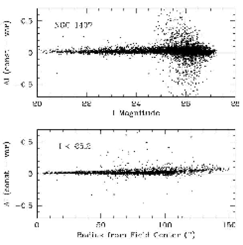
Figure 2: (Upper panel:) Comparison of photometry for a constant PSF versus a PSF with quadratic dependence on field location $x,y$. For the NGC 1407 $I-$band image, the difference between the two measurements is plotted against $I$ magnitude. The enhanced scatter near $I\sim 26$ is due mainly to very faint objects near the galaxy center where the background light is high. (Lower panel:) Difference plotted versus radius from the center of the ACS/WFC field, in arcseconds. Most of the stars follow a trend of gradually increasing $\Delta I$ with radius; a more thinly populated “second sequence” sitting at higher $\Delta I$ belongs to stars located along one particular radial direction (detector corner).

We defined the point spread function empirically for each frame, using anywhere from 50 to 80 “stars” distributed across the frame (as noted above, many of these are bright globular clusters, with measured FWHMs of $2.1-2.5$ px, a range similar to that generated by the field dependence of the PSF). The candidates were manually selected to be bright and uncrowded. Initially we ran trials for (a) a constant PSF (i.e. the same everywhere on the frame), (b) a PSF linearly variable in $x$ and $y$, and (c) a PSF quadratically variable in $x$ and $y$. The quality of fit across the images was marginally but noticeably best with the quadratically variable PSF, though it produced very little difference in the measured magnitudes of the objects anywhere in the field. A sample of these tests is shown in Figure 2. No trend with magnitude between the two types of PSFs is apparent, and only a slight trend with field location, reaching a center-to-edge amplitude $\simeq 0.05$ mag at the corners of the frames. (The very slight zeropoint offset between the two PSF scales is not significant, since it is routinely removed during the aperture-correction stage).

For each galaxy, we constructed a master finding list of objects by reregistering and stacking all the available multidrizzled frames in both colors, and running daophot on the summed frame. Then, we carried out allstar with the master candidate list on each of the $B$ and $I$ frames, keeping only objects that appeared on all frames; this step rejected virtually all remaining cosmic rays and other artifacts that might have crept through the Multidrizzle preprocessing, as well as any objects with extreme colors.

Lastly, we have avoided any objects located within $5^{\prime\prime}$ of the galaxy nuclei, because of the bright background light there. This region corresponds typically to a linear radius less than 1 kpc for our target galaxies, and has little effect on any of the following discussion.

2.2 Calibration Steps

Following the prescriptions in Sirianni et al. (2005), we used bright starlike objects (essentially, the bright clusters used to define the PSF) on each frame to determine the mean “aperture correction”, which is the difference $(m_{psf}-m_{10})$ between the psf-fitted magnitude and the magnitude measured through a 10-pixel-radius ($0\farcs 5$) aperture. We then extrapolated from $0\farcs 5$ to “infinite” radius subtracting the values recommended by Sirianni et al. ($\Delta B=0.107,\Delta I=0.087$ mag). In summary, the measured magnitudes on the natural VEGAMAG filter systems are then

$$F435W=b_{psf}+\Delta B_{ap}-0.107$$ (1)

$$F814W=i_{psf}+\Delta I_{ap}-0.087$$ (2)

where $b,i_{psf}$ are the magnitudes measured by daophot/allstar, normalized to an exposure time of 1 second, and $\Delta B,I$ are the corrections to an aperture magnitude of radius 10 pixels.

The last step is to convert the instrumental magnitudes to standard $B$ and $I$. We have adopted the synthetic model prescriptions from Sirianni et al. (2005) for objects in the color range $(B-I)>1$, which we repeat here:

$$F435W=B-25.749-0.008~{}(B-I)+0.005~{}(B-I)^{2}$$ (3)

$$F814W=I-25.495+0.010~{}(B-I)-0.006~{}(B-I)^{2}$$ (4)

Iteration of these relations quickly converges to a final pair of $B,I$ magnitudes, since the color terms in the transformations are very small.

We have not applied any CTE (charge transfer efficiency) corrections to the raw photometry. Because these images are relatively long exposures with broadband filters, and are located in the outskirts of bright giant galaxies, the ambient sky background is high enough that CTE corrections are expected to be 0.02 mag or less for all our data (Riess &Mack, 2004).

Combining all the calibration steps, we believe our $B$ and $I$ zeropoints are likely to be uncertain from one galaxy to another by $\pm 0.02-0.03$ mag each. The dominant sources of error are the aperture corrections ($\Delta B,\Delta I$), the extrapolations to infinite aperture radius, and the zeropoints in the final transformation equations, each of which appear to have potential systematic uncertainties of $\pm 0.01-0.02$ mag. In addition to these calibration uncertainties, the external uncertainties in the foreground reddenings of the galaxies in our survey are at the level of $\Delta(B-I)\sim\pm 0.02$ mag. These small potential shifts are what place ultimate limits on the degree to which we can intercompare the $(B-I)$ distributions even within one strictly homogeneous dataset.

2.3 Aperture vs. PSF Photometry

To test the robustness of the color-magnitude data to the details of the photometric procedures, we have extensively compared the allstar PSF-fitted data with magnitudes measured directly from small-aperture photometry. The main advantage of aperture photometry is that it provides a simple measure of the total light within a fixed radius and is less affected by small object-to-object differences in the actual profile shape. The compensating advantage of PSF fitting is that it is less affected by crowding. For the very faintest objects, PSF fitting through allstar is also less subject to the occasional “wild” excursions in measured magnitude that can affect aperture photometry due to combinations of noise in both the star and sky annuli, crowding, and centering uncertainties. For this comparison, we used a 3-pixel aperture radius (similar to the PSF fitting radius) and calibrated it to the absolute $B$ and $I$ magnitude scales with the same techniques described above.

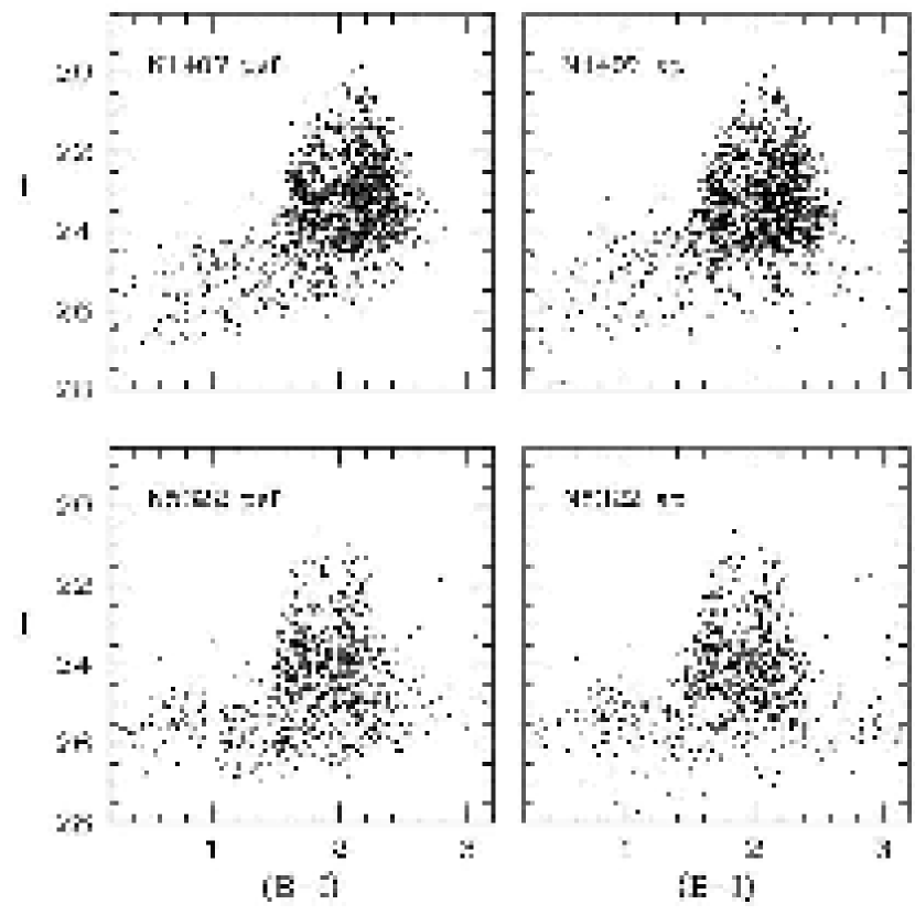
Figure 3: Color-magnitude plots for the measured objects around NGC 1407 (top) and NGC 5322 (bottom). In each pair of plots the left panel shows the photometry measured via allstar PSF profile fitting, while the right panel shows the same objects measured through fixed-aperture photometry of 3 pixels radius. No corrections for reddening have been applied to the data. The objects in the approximate color range $1.4<(B-I)<2.6$ are in the expected range for old globular clusters.

In Figures 3 to 6, we show the color-magnitude plots in $(I,B-I)$ for all eight of our BCGs, with both PSF-based allstar photometry and with small-aperture photometry. In each pair of graphs the PSF photometry is shown on the left, and the aperture photometry of exactly the same set of objects on the right.

The main point we draw from this comparison is that the two methods give extremely similar color-magnitude distributions, essentially because of the fundamental advantage that crowding is not a major problem in any of these fields. In each galaxy field, the brighter part of the color-magnitude array is populated by a pair of near-vertical sequences in the color range $1.4<(B-I)<2.6$ that are the red and blue globular cluster populations. The detailed characteristics of these sequences will be discussed in later sections. In all the diagrams the main contribution from field contamination comes in at faint, blue levels ($I>25,(B-I)<1.5$); although contamination from similarly faint red objects must exist, these objects are mostly cut off by the faint-end incompleteness in the $B$ images and thus do not appear in the diagrams.

We find no systematic differences in magnitude or color between the two methods larger than the $\pm 0.02-$mag calibration uncertainties discussed above. As expected, the aperture-based photometry tends to show (a) a few more “outliers” at very red or blue colors produced by occasional crowding; and (b) a very slightly larger color spread in the red and blue cluster sequences. For these reasons, we prefer to use the PSF-based photometry in the rest of our discussion.

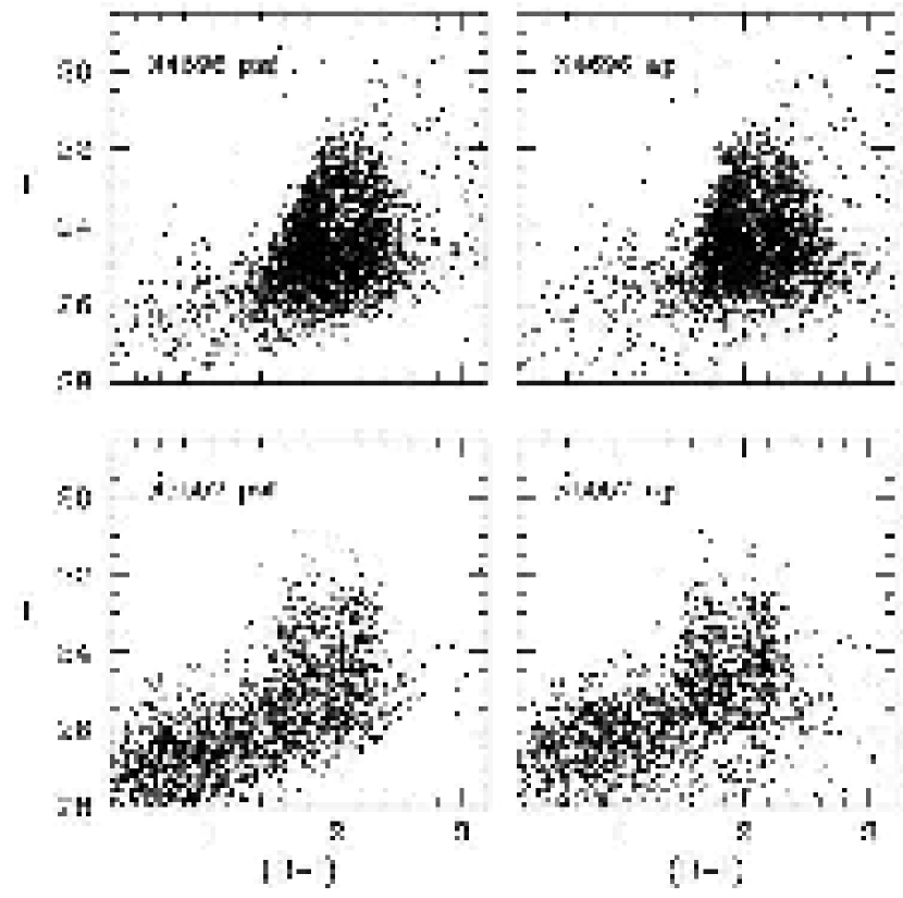
Figure 6: Color-magnitude plots for the cluster populations around NGC 4696 (top) and NGC 5557 (bottom).

The single exception to this choice is the NGC 4696 field, which is the one with the largest measured number of clusters in our survey. Close inspection of Figure 6 shows a second-order effect on the mean colors for objects fainter than $I\sim 23.5$. Within the PSF-based photometry, the average color of the cluster population becomes slightly and progressively bluer toward fainter magnitudes, whereas in the aperture photometry the mean colors of the cluster sequences remain constant with magnitude over that $I$ range. We have not been able to find a definitive explanation for this small but puzzling trend in the PSF photometry for this one field, but it may be due either to (a) higher-order nonuniformities in the PSF shape across the frame that we have not been able to track, or (b) small differences among the true radii of the clusters (thus their true profile widths). Fully accounting for this residual effect will require much more extensive and painstaking object-by-object photometry. For the present, we have chosen to use the aperture-based photometry for NGC 4696 in the discussion that follows. For the other galaxies, we use the PSF data. As will be seen below, however, much of our discussion is based on the brighter clusters in the color-magnitude data and thus is little affected by this particular issue.

2.4 Conversion of Color to Metallicity

Although the $(B-I)$ index is one of the most effective ones for GCS metallicity estimation that can be constructed from commonly used broadband filters, it has only rarely been employed before in GCS studies (Couture et al., 1990; Grillmair et al., 1999; Whitlock et al., 2003; Jordan et al., 2004). A necessary preparatory step for our analysis is to define a conversion from color to metallicity, and although the globular clusters in the Milky Way are not guaranteed to be identical to those in giant ellipticals, they remain our best resource for defining the conversion. In Figure 7, we show the catalog data (Harris, 1996) for 95 Milky Way clusters with known $(B-I)$, spectroscopically measured [Fe/H], and foreground reddenings less than $E_{B-V}=1.0$. We adopt a linear conversion

$$(B-I)_{0}=(2.158\pm 0.068)+(0.375\pm 0.049)~{}[Fe/H]$$ (5)

shown by the solid line in the Figure. The uncertainty in the slope is such that for the very reddest or bluest clusters, the deduced [Fe/H] could be systematically in error by $\pm 0.1$ dex. In addition, any cluster metallicities higher than Solar require extrapolation of the relation and thus are only estimates.

3 The Color-Magnitude Data

In Figures 3 to 6, the $I$ vs. $(B-I)$ scatter plots (color-magnitude diagrams or CMDs) for all eight BCGs are shown. The first and most obvious features to emerge from these plots are that (a) the GCS populations stand out clearly in all the galaxies as the vertical sequences within $1.4<(B-I)<2.6$, (b) the color distributions are strongly and unequivocally bimodal in all the galaxies, and (c) the relative numbers of blue and red clusters differ noticeably from one galaxy to the next. We will quantify these characteristics in the following discussion, but at this point it is simply worth noting that the promise held out by using the combination of ACS/WFC with long exposure times and with the $(B,I)$ filters has been fulfilled, removing all the problems associated with the previous, more limited $(V-I)$ studies. The blue and red sequences are more clearly separated in these new data than in all but the best photometry in the previous literature, and as will be shown below, the internal dispersions in each sequence are well resolved.

3.1 Estimates of Field Contamination

Field contamination of the CMDs – that is, the residual presence of foreground field stars and very faint, compact background galaxies that succeeded in passing through the photometric procedures – is clearly at a low level, at least for the brighter parts where the cluster sequences stand out the most strongly. At fainter levels (corresponding to $M_{I}>-9$ in rough terms), large numbers of faint blue objects populate the diagrams; similarly faint but red objects are visible in the $I$ images, but they are cut off by the detection incompleteness in the $B$ frames and thus do not appear in our two-color data. However, the data at these fainter levels are of no interest in our present discussion and are not used here in any way. They are more relevant to the derivation of the globular cluster luminosity functions (GCLF) which will be the subject of a future paper.

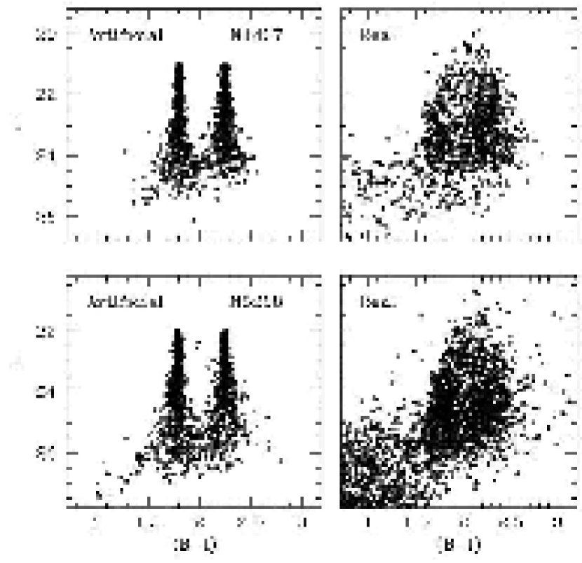
Figure 11: Artificial addstar tests for internal measurement errors of the photometry. Upper panels: Measured magnitudes and colors for the artificial stars inserted into the NGC 1407 field, compared with the actual measured data. The added stars all fall along lines exactly at $(B-I)=1.80$ and 2.25, and are added in equal numbers per unit magnitude. No attempt has been made here to match the intrinsic luminosity function of the real globular clusters. Lower panels: The same data tests for the NGC 3268 field.

The magnitude and color ranges of interest for our present work are the ones which bracket the brighter globular clusters, $-13<M_{I}<-9$ and $1.4<(B-I)_{0}<2.4$ (see especially Figure 11 later in the paper for CMDs plotted in $(M_{I},(B-I)_{0})$). This is the region for which we are more directly interested in the level of contamination. To quantify the true number of contaminating objects very exactly, we would need to have remote-background fields to refer to, but these are not on hand. Color-magnitude plots of each field subdivided by galactocentric radius also show that the globular cluster sequences are prominent even out to the edges of the ACS camera field. That is, the GCSs in these supergiant galaxies extend detectably well past the borders of our fields, so that we cannot use the outer parts of the frames to set anything but the most generous (and in practice, useless) upper limits on the field contamination.

What we have done instead to estimate the level of contamination is to refer back to the color-magnitude diagrams themselves. We use the numbers of stars that appear in the same luminosity range ($-13<M_{I}<-9$) as the brighter globular clusters, but at bluer or redder colors than the one-magnitude range ($1.4<(B-I)_{0}<2.4$) that encloses the globular clusters. If we then assume more or less arbitrarily that field stars are evenly spread in color over the wider range $\simeq 0.8-3.2$ in $(B-I)_{0}$, then the counted number of stars per unit magnitude will give a plausible estimate of the contamination level within the globular cluster sequences.

The results of this numerical exercise are shown in Table 2. The successive columns give (1) NGC number, (2) total number of globular cluster candidates in the range $-13<M_{I}<-9$ and $1.4<(B-I)_{0}<2.4$; (3) estimated number of contaminants in the same range, from the number of bluer and redder objects present in the CMD; and (4) the ratio $N_{c}/N_{f}$. It is clear from these numbers that the contamination level is only a few percent for most of the fields, reaching a maximum of 11% for the sparse NGC 7049 GCS. We conclude that we can safely analyze the color distributions of the candidate GCS populations without field contamination corrections.

3.2 Bimodality Model Fits

The raw color-magnitude diagrams for the eight BCGs can now be used to determine more quantitative features of the color/metallicity distributions of the globular clusters. The first and most basic issue is to determine how strongly a bimodal fit is preferred at any level in the CMDs over simpler models such as a unimodal distribution. This question is easily answered for most of the visible luminosity range, but less so at the faintest levels in our data where the red and blue sequences become lost in increasing measurement errors and field contamination, and also at the top end (discussed especially in the following section).

Unlike the custom in many previous studies, we do not assume equal dispersions in these KMM fits for the blue and red subpopulations; such an imposition on the data is unjustified when the data are of high enough quality to resolve differences between the modes.

In Figure 8, we show the results of this exercise where we have combined all eight BCGs into a single color-magnitude distribution in $(M_{I},(B-I)_{0})$, and divided the combined list into narrow luminosity intervals such that precisely 200 objects are in each bin. The upper panel of the Figure shows the probability $p$ given by the KMM fitting code that the color distribution can be matched by a single Gaussian curve. For all luminosities $M_{I}>-10.5$, we find log $p$ $<-3$ and the null hypothesis of unimodality can therefore be strongly rejected. Two other features of this graph, however, are worth noting: first, for $M_{I}>-9.5$ the value of $p$ slowly increases towards fainter levels from $\sim 10^{-10}$ to $10^{-4}$. This trend shows the increasing effects of photometric measurement scatter and some field contamination that tend to make the blue and red modes spread out and partially overlap. Second, for the upper range $M_{I}<-10.5$, a few of the bins have probability levels $p>0.01$, which means that a unimodal-Gaussian fit to the color distribution starts to become a plausible (though still not convincing) fit. This effect cannot be attributed to either photometric scatter or field contamination, and must be regarded as real. This particularly interesting top end of the CMDs will be discussed in more detail in the next section.

The lower panel of Fig. 8 shows (solid line) the trend of $f$(blue), the fraction of clusters that the KMM fitting routine assigns to the blue mode (and where by definition $f$(red) $\equiv 1-f$(blue)). If the clusters in both modes have intrinsically similar mass distributions, then we would expect to see little systematic change in this ratio with luminosity. Indeed, little if any significant change in the ratio takes place, with on average about 55% of the whole GC sample falling into the blue, metal-poor mode. Lastly, in the same figure, the dashed line shows the color difference $\Delta\langle B-I\rangle$ between the peaks of two fitted Gaussian curves. This difference shows no change with luminosity for $M_{I}>-9.5$, but above that it steadily decreases toward higher luminosity, indicating that the two fitted modes are gradually converging toward the top end (see below).

3.3 Mean Colors and Dispersions

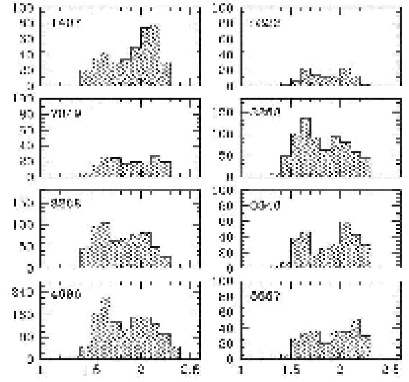
Figure 9: Histograms in color for the globular cluster systems. Here, the number of objects per 0.1-mag bin in $(B-I)_{0}$ in the luminosity range $-10.5<M_{I}<-9.0$ is shown for each galaxy. All the distributions show the basic phenomenon of bimodality.

The dereddened color histograms derived directly from the color-magnitude plots are shown for each galaxy in Figure 9. Here, we use only the objects in the specific luminosity range $-10.5<M_{I}<-9.0$; as we note above, the faint end is set to minimize effects of field contamination as well as the spreading effect of photometric random errors. The bright end is set for reasons that were hinted at above, indicating that this upper end requires special treatment. We have used these histograms to determine parameters for best-fit double Gaussian curves derived by both a maximum-likelihood method through the KMM mixture modelling routine (Ashman et al., 1994), and independently by a separate nonlinear least-squares Levenberg-Marquardt code. The results from these two independent codes agreed closely, and we will refer to only the KMM fits below.

One of the first points to emerge from our new MDFs is that the red population consistently displays a significantly bigger color dispersion (thus metallicity range) than the blue population. In Table 3, we list the parameters of the resulting fits, as well as the fitted ratio of total subpopulations $(N_{blue}/N_{red})$, and the color difference $\Delta\langle B-I\rangle$ between the red and blue modes as defined above. The mean values over the eight galaxies are listed at the bottom of the Table, along with the galaxy-to-galaxy rms dispersions (in parentheses).

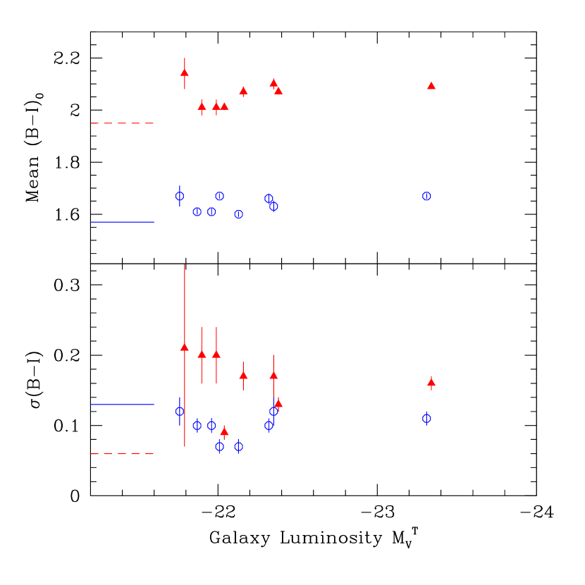
Figure 10: Parameters for the double-Gaussian fits to the color histograms in Figure 8, with data from Table 3. The Gaussian peaks $\langle B-I\rangle_{0}$ and standard deviations $\sigma_{B-I}$ of the red and blue modes are plotted versus galaxy luminosity. Points for the blue (low-metallicity) clusters are the open circles and the red (high-metallicity) clusters are the filled triangles. The error bars in the upper panel show only the internal uncertainty of the mean and do not include the uncertainty in the foreground reddening of the galaxy itself. The mean and standard deviation for the metal-poor Milky Way globular clusters are indicated by the solid lines, while the metal-rich Milky Way clusters are shown by the dashed lines. Note that the metal-rich Milky Way clusters form a considerably narrower subpopulation (smaller $\sigma$) than any of the giant ellipticals.

The means and standard deviations are displayed in Figure 10. Direct application of Eq. (5) yields mean metallicities of $\langle Fe/H\rangle_{blue}=-1.30\pm 0.10$ and $\langle Fe/H\rangle_{red}=-0.25\pm 0.10$, along with mean intrinsic dispersions $\sigma$[Fe/H] $=0.32$ dex (blue) and 0.43 dex (red).

For comparison, in Table 2 and Fig. 10 we show the values for the red and blue cluster populations in the Milky Way. [Fe/H] data from Harris (1996) were used to find the best-fit means and dispersions in metallicity, and these were translated into equivalent $(B-I)$ values through Eq. (5). For the Milky Way, the blue population is characterized by $\langle$Fe/H$\rangle=-1.56\pm 0.04$, $\sigma_{[Fe/H]}=0.34\pm 0.04$, and the red population by $\langle$Fe/H$\rangle=-0.55\pm 0.04$, $\sigma_{[Fe/H]}=0.16\pm 0.03$. The red populations in the giant ellipticals are more metal-rich, and cover a very much broader range, than their counterpart in the Milky Way. Furthermore, the mean abundance of the blue clusters in the BCGs is consistently $0.1-0.2$ dex more metal-rich than in the Milky Way. As has also been discussed elsewhere (Strader et al., 2004; Woodley et al., 2005), this comparison provides partial evidence that these BCGs cannot have assembled only from mergers of pre-existing galaxies the size of the Milky Way or smaller, even with the addition of more metal-rich clusters formed from gas in the mergers.

A correlation between the peak color of the blue and red modes and parent galaxy luminosity has been found (see, e.g. Forbes et al., 1997; Forbes & Forte, 2001; Strader et al., 2004, for recent discussions) in the sense that more luminous galaxies on the average have redder GCs of both types. However, all the galaxies in our sample are at the high-luminosity end of this sequence, so the galaxy-to-galaxy differences in GCS color are expected to be small. In fact, we find no evidence at all in our sample that the blue clusters differ in mean color from one galaxy to the next: the measured dispersion of $\pm 0.03$ mag in the mean color $(B-I)$ (Table 2) can be completely explained by the combination of internal zeropoint scatter in the photometry and the external uncertainties in the foreground reddenings (both of which are typically $\pm 0.02$ mag). Furthermore, their internal color range $\sigma_{B-I}$ has a galaxy-to-galaxy dispersion of just $\pm 0.02$ mag.

For the red clusters, the dispersion in mean color is $\pm 0.05$ mag, and the range in $\sigma_{B-I}$ is $\pm 0.04$ mag, hinting at somewhat larger intrinsic variation than the blue population. Although our sample of BCGs is small, the characteristics of the red clusters do not obviously correlate with any other properties of their parent galaxies, such as luminosity or surrounding environment. As will be discussed later, if the red population formed primarily from the last few major starbursts that built the majority of the galaxy, then its characteristics could well be subject to large stochastic variations.

4 Artificial-Star Tests

To determine the effects of pure measurement scatter on the globular cluster color distributions, we carried out a series of artificial-star tests on the images. These were done in the usual way with daophot/addstar by adding scaled PSFs at random locations in the $B$ and $I$ images of each galaxy. The added stars were defined to lie along vertical dispersionless sequences at $(B-I)_{0}\simeq 1.65$ and $(B-I)_{0}\simeq 2.05$, covering the range of magnitudes occupied by the real globular clusters in the image. Typically we add 500 to 1500 artificial stars at a time; these do not add noticeably to the crowding level of the frames, since all of them are very uncrowded in any absolute sense. We then measure the synthesized $B,I$ images with exactly the same daophot procedure as before, and find out how many of the added objects are recovered and at what magnitudes.

Some sample results are shown in Figure 11, for NGC 1407 and 3268. The results for the other fields look very similar, because the exposure times were planned to yield very much the same photometric limits in absolute magnitude $M_{I}$ in the globular cluster luminosity function. Since crowding effects are negligible, the measurement scatter in the colors is generated almost entirely by the background image noise and photon statistics. No bias (systematic error) is present at any magnitude level of interest, and for the brightest $\sim 2-3$ mag of the globular cluster distribution, the measurement scatter is far less than the observed dispersions in color for both the blue and red populations. These tests provide strong evidence that we are fully resolving the true color spreads of both the red and blue populations of clusters.

The artificial-star tests were also used to evaluate the completeness $f$ of the photometry. We define $f$ as the number of artificial stars inserted with addstar in a given narrow magnitude range that were found and measured, divided by the number actually inserted in that magnitude bin. To be labelled as successfully “found”, a star had to be recovered in both $B$ and $I$. Over the range of magnitudes that we are using in this paper to discuss the metallicity distribution (and excluding the innermost $5^{\prime\prime}$ regions around each galaxy center as noted above), our photometry is highly complete ($>95$%) and the MDFs unaffected by bias.

5 The Brightest Globular Clusters in the MDF: A New Feature

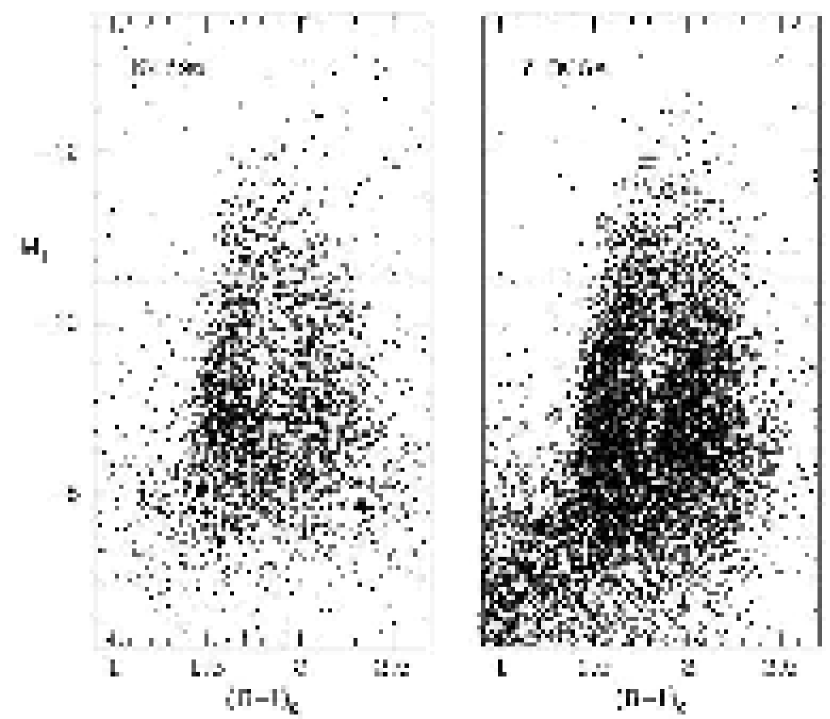
Figure 12: Left panel: Expanded color-magnitude diagram for the GCS in NGC 4696, the single largest cluster population in our survey. The dashed line is at $M_{I}<-10.5$. Right panel: Color-magnitude diagram for the GCSs in the other 7 galaxies in our survey, normalized to absolute magnitude and intrinsic color and combined. The three open stars mark the locations of massive Local Group globular clusters NGC 6715, $\omega$ Centauri, and (at top) M31-G1.

While plotting up the color-magnitude array for NGC 4696, which is the galaxy with the largest single cluster sample in our survey, we noticed a new feature of the MDF: for magnitudes more luminous than $M_{I}\simeq-10.5$ (corresponding to $I<23$), the distribution of cluster colors does not appear strongly bimodal, unlike the very obvious bimodality at fainter levels. The effect is somewhat as if the distinct blue and red modes that dominate at lower luminosities simply merge together as they go up to higher luminosity. In Figure 12 the data are shown on a bigger scale, with the approximate dividing line $M_{I}=-10.5$ below which bimodality is clearly evident. This line is not meant to imply an abrupt transition (indeed, the trends shown in Fig. 8 indicate a smooth, gradual changeover), but only a guide to the point where this effect starts to take place.

We then looked for the same feature in the other galaxies. Though all the rest have smaller observed sample sizes, the same characteristics can be seen, and more prominently in the galaxies with larger measured GCS populations. The composite color-magnitude distribution for the seven other galaxies combined is also shown in Fig. 12, which comprises a sample twice as large as in NGC 4696 alone. The same feature shows up. For the most luminous globular clusters, either the bimodality of the MDF disappears, or else the two modes overlap so closely that they can no longer be cleanly distinguished.

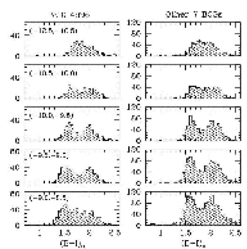
Figure 13: Left panel: Histogram for the globular clusters in NGC 4696, derived from the previous figure and divided into $M_{I}$ absolute magnitude bins as labelled. Right panel: The same distributions for the other seven BCGs combined. For $M_{I}<-10.5$ the clusters follow an increasingly unimodal color distribution.

Color histograms for NGC 4696 and the other seven galaxies, subdivided by magnitude, are in Figure 13, showing the trend for bimodality to weaken at higher luminosities. The tests of the photometry described in the previous section show that it is not the result of any purely internal effects such as crowding, saturation, incompleteness, measurement bias, field contamination, or differences between PSF and aperture photometry.

5.1 Statistical Tests

Is this “top end” of the cluster distribution actually a broad, unimodal distribution in color? The tests of the KMM bimodal fitting on the composite sample described previously suggest that it is more likely to be the result of the two modes (blue and red) that are very distinct at lower luminosities, but that converge at higher ones. But to investigate this further, we have applied the same KMM mixture modelling tool as described earlier to the individual galaxies, in order to test how well the luminous region ($M_{I}<-10.5$) can be matched by a single Gaussian distribution. Our key numerical results are in Table 4. In the Table, columns (2) and (3) give the probability $p$ that a single Gaussian fits the MDF satisfactorily in the $M_{I}$ range $(-13.5,-10.5)$, followd by the number of clusters in that luminosity bin. Columns (4) and (5) give the same numbers for a slightly fainter range $(-9.8,-9.5)$ that has almost the same sample size as the top end, so that the two probability values can be compared directly. Finally, columns (6) and (7) for completeness give these same numbers for the much broader range $(-10.5,-9.0)$. We conclude that for all the galaxies, the MDF is very clearly bimodal in that fainter range. Blank entries are ones for which the KMM fit did not converge.

We look now particularly at the results for the bright end. The smallest samples (such as for NGC 7049 with 45 bright clusters, or NGC 3348 with 66) return tolerably large $p-$values, indicating that a unimodal Gaussian provides an adequate fit. In general, however, the probability $p$ becomes lower as sample size increases, which is exactly the result expected if the underlying distribution requires more than a single Gaussian to fit it. At the same time, for all the galaxies the $p-$value decreases dramatically for the fainter bin (the second pair of numbers in the Table) compared with the brighter bin, even with the same sample size. All these results are entirely consistent with the interpretation that the MDF is intrinsically bimodal, but that the two modes do overlap more closely at progressively higher luminosity.

As a concluding point of discussion, we return to the original question: is the MDF for the luminous ($M_{I}<-10.5$) clusters actually unimodal? It is trivially true, but nevertheless worth restating, that the KMM fitting test does not answer that question. Instead, it answers a much more restricted question: it gives the probability that a single Gaussian function matches the distribution. But there is no underlying physical reason why the globular cluster MDF should obey a Gaussian or double-Gaussian form: different chemical evolution models and cluster formation models can be found in the literature that are all physically based, and that produce non-Gaussian but unimodal MDFs. An intrinsically unimodal distribution might be asymmetric, or more sharply peaked than a Gaussian, or broader and flatter. In all these other cases, any statistical fitting code that uses Gaussian functions will require two or more such functions to generate an adequate fit to the data even though the underlying shape of the actual MDF has a different nature.

As most previous authors have done, we regard the KMM Gaussian-based fits only as guides that provide useful numbers to quantify the mean colors and intrinsic dispersions of the blue and red cluster populations. In our view, the main argument that the MDF has a bimodal form at all luminosity levels is the gradual trend with $M_{I}$ that was presented in Section 3 above. That is, the “transition point” at $M_{I}\simeq-10.5$ does not mark any kind of abrupt change from bimodal to unimodal; it simply marks the luminosity at which the two modes begin to overlap strongly (see also Strader et al., 2005). We will quantify the global trend in color with luminosity below, and suggest an interpretation for it.

5.2 Is This a Universal Phenomenon?

Viewed with the benefit of hindsight, exactly the same feature at the bright end of the MDF – a merging of the bimodal distribution into a broad unimodal one – can be seen in some other galaxies from the data in the literature. Ostrov et al. (1998) first remarked that the brightest clusters in NGC 1399 appeared to show a broad, unimodal color distribution in $(C-T_{1})$, splitting into a bimodal distribution fainter than $T_{1}=21$ (roughly equivalent to $M_{R}=-9.9$, very similar to the crossover level we have identified). Dirsch et al. (2003), from a more extensive photometric study of NGC 1399 again in $(C-T_{1})$, concluded the same thing (see especially their Figure 11). In NGC 5128, a clear hint of this feature can be seen in the $(C-T_{1})$ color-magnitude distribution shown by Harris, Harris, & Geisler (2004); although the cluster sample in this case is not large, it is biased strongly towards the brightest objects by observational selection and so the top end is covered fairly well. And in M87 a hint of this same feature may also be seen in the WFPC2 observations of Whitmore et al. (1995) and Larsen et al. (2001), though both the sample size and metallicity sensitivity of the $(V-I)$ index used there are too low to make it unambiguous.

Notably, all three of these other galaxies are BCGs: M87 in Virgo, NGC 1399 in Fornax, and NGC 5128 in the Centaurus group. The question immediately arises whether this intriguing characteristic of the MDF is peculiar to these central giant galaxies, and if so, why? There is not yet enough evidence to start answering this question. Large samples of clusters, and a metallicity-sensitive color index, are both needed for this kind of MDF analysis to be done. In other words, if the bright-end “merging” of the MDF modes is a universal feature of GCSs, the reason we see it prominently in BCGs may simply be a result of the sheer size of the cluster populations that they hold. The bright-end clusters are rare to begin with, so that in smaller galaxies with fewer clusters in total, it would not be possible to subdivide the MDF by magnitude without losing out to small-number statistics. Many systems would have to be co-added to regain statistical significance and look for the effect.

But some counterexamples to the simple population-size explanation may already exist, such as in the Virgo system NGC 4472 (M49), a giant E galaxy comparably luminous with M87 but not at the center of the entire Virgo cluster. Two recent photometric studies with wide-field coverage and large statistical samples of the GCS (Geisler et al., 1996; Rhode & Zepf, 2001) plainly reveal the metal-rich and metal-poor modes in the color-magnitude distributions of the clusters, and yet both studies indicate that the two modes remain fairly distinct at the high-luminosity end. Thus a very tentative suggestion from this one comparison is that the phenomenon we have isolated may indeed be associated most strongly with cluster formation in the deep potential wells of the brightest central giant galaxies. This argument provides additional reasons to look for the phenomenon in small galaxies of other types. An excellent prospect for doing such a test would be with the ACS Virgo Cluster Survey (Côté et al., 2004) of a hundred normal galaxies covering a wide range of luminosities.

Recently Strader et al. (2005) have discussed ACS $g^{\prime}z^{\prime}$ photometry of the cluster populations around several galaxies including the Virgo giants M87, NGC 4472, and NGC 4649. The $(g^{\prime}-z^{\prime})$ color index has a metallicity sensitivity very similar to $(B-I)$, allowing the blue and red MDF modes to be clearly identified in their GCS populations. They find that for M87, and possibly also in NGC 4649, the blue-cluster mode becomes progressively redder at higher luminosity, basically the same trend we find here. In NGC 4472, they find no such trend, in agreement with the previous studies cited above. The advantage of their dataset is that it is internally homogeneous and contains a wide variety of E galaxies; their results are consistent with our suggestion that the color/luminosity phenomenon is associated with central giant ellipticals.

We note that Ostrov et al. (1998) and Dirsch et al. (2003) described the bright clusters in NGC 1399 as displaying a unimodal color distribution, whereas Strader et al. (2005) state that the blue clusters in M87 follow a color/luminosity trend. Our view is that these two descriptions are both results of one and the same phenomenon.

5.3 Mass Fractions

In our combined material for all eight galaxies, there are almost 4600 globular clusters brighter than $M_{I}=-9.0$ (Table 2). If as noted earlier the GCLF has a normal Gaussian-like shape with turnover at $M_{I}=-8.4$ and dispersion $\sigma\simeq 1.4$ magnitudes (Harris, 2001), then the total GCS population we are drawing from in all eight galaxies, and within the ACS field of view, is nearly 15000 clusters. A total of 970 of them, or just 6.5%, are brighter than $M_{I}=-10.5$. But even though the clusters brighter than this dividing line are rare, they contribute a large fraction of the total mass in the system: $M_{I}=-10.5$ corresponds to $L=5\times 10^{5}L_{\odot}$, or $M=1.5\times 10^{6}M_{\odot}$ for a visual mass-to-light ratio of 3. With the GCLF parameters as noted above, and with the assumption that the cluster mass-to-light ratio is roughly independent of luminosity, then the clusters brighter than $M_{I}=-10.5$ make up a full 40% of the total mass that is now in the GCS. In other words, they are major players in the formation history of star clusters, using up a significant fraction of the gas that was eventually incorporated into bound clusters during the galaxy formation era.

In the Milky Way (Harris, 1996), there are two globular clusters known which clearly belong to this high-mass regime: $\omega$ Centauri at $1.0\times 10^{6}L_{\odot}$ and NGC 6715 at $0.8\times 10^{6}L_{\odot}$. A few more are known in M31, the most notable of which is M31-G1 (Meylan et al., 2001) at $2.3\times 10^{6}L_{\odot}$. The positions of these local examples are shown for comparison in Fig. 12. In our entire sample, the brightest single objects can only be identified statistically since the numbers trail off indistinctly with luminosity (see again Fig. 12), but the top end appears to be near $M_{I}\simeq-12.6$, equivalent to more than 12 million Solar masses. M31-G1 particularly is near the very maximum of the mass range that globular clusters reach in the real universe.

5.4 Image Morphologies and Spatial Distributions

An immediate question is whether or not the brightest GCs we see around our target galaxies are somehow different in any obvious way from the fainter “normal” ones, possibly indicating a different type of origin. For example, the Ultra-Compact Dwarfs (UCDs) (Phillipps et al., 2001; Drinkwater et al., 2003) have comparable luminosities to the brightest GCs, small linear sizes, and could be the remnant nuclei of disrupted dE’s. Such objects could help populate the bright end of our GCS luminosity distribution (see Mieske et al., 2004, for a recent example). Another recently discovered type of cluster-like object is W3 in NGC 7252 (Maraston et al., 2004), which has both a remarkably high mass ($8\times 10^{7}M_{\odot}$) and an effective radius (18 pc) several times larger than a typical globular cluster.

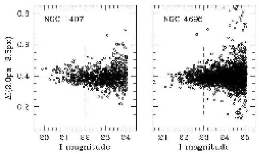
Figure 14: Tests for nonstellarity of the bright globular clusters. The left panel shows the magnitude difference $\Delta I$ between a 2-px and 3.5-px aperture radius versus $I$ magnitude for the globular clusters around NGC 1407, the nearest galaxy in our survey. The horizontal line shows the mean value for starlike objects (ones matching the PSF profile accurately), while the vertical dashed line shows the approximate dividing line at $M_{I}=-10.5$ from Figure 10. Ones fainter than $I\simeq 22$ define a bimodal MDF, while brighter ones define a unimodal MDF. Some of the clusters in the brighter part are visibly nonstellar, scattering up to higher $\Delta I$. The right panel shows the same distribution for NGC 4696, a galaxy twice as far away (see text).

If any of the brightest GCs are of this type, then they might have more extended structures than normal clusters. We have looked for evidence of this effect. A simple tracer of nonstellarity is the magnitude difference between two small apertures of different radii; two examples are shown in Figure 14. Here the magnitude difference in $I$ between a 2-pixel-radius aperture and a 3.5-pixel aperture is plotted against magnitude. Nonstellar objects will have more extended wings than the point spread function and thus sit above the main distribution defined by objects that match the PSF well.

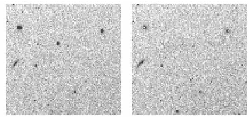
Figure 15: Left panel: A $22^{\prime\prime}$ wide segment of the halo region around NGC 1407, the nearest BCG in our survey. The three bright objects in the top half of the image are globular clusters in the “unimodal”, bright-end part of the metallicity distribution function. Right panel: The same field after the point spread function has been subtracted from the profiles of the three objects. Note that the middle one is nearly starlike and subtracts cleanly, but the other two have left residual faint envelopes. The fainter objects in the lower half of the frame are all starlike.

For NGC 4696, at a distance of 42 Mpc, Fig. 14 shows only the horizontal starlike sequence, with no strong evidence for any very extended objects. At this distance, the FWHM of the PSF (2.2 px) corresponds to a diameter of 25 parsecs (for comparison, $\omega$ Cen has a half-light diameter of 13 pc and the UCDs have sizes similar to this or a bit larger). Most of the galaxies in our list are at similar distances (Table 1) and give similar results. However, for the closest galaxy in our survey, NGC 1407 at d = 23 Mpc, clusters the size of $\omega$ Cen or bigger would subtend half-light diameters of 2.2 px and thus should be marginally resolved. In fact, we find a population of about 20 to 30 bright objects around NGC 1407 that are slightly more extended than the starlike sequence: in Fig. 14, these are the ones with $\Delta I\geq 0.4$, $I<21.5$. Inspection of the images shows that faint extended envelopes are present around several of them; for the sake of visual comparison, we show three of these in Figure 15. Such objects have morphologies very similar to the way $\omega$ Cen would look at that distance.

At the same time, few if any objects that are significantly more extended in morphology show up in our data. Although this should in large part be a selection effect (faint objects with extremely different sizes than the image PSF will tend to be rejected in the photometry), it verifies that essentially all the objects in our samples can be considered as bona fide globular clusters of the range of properties we have already seen within the Local Group.

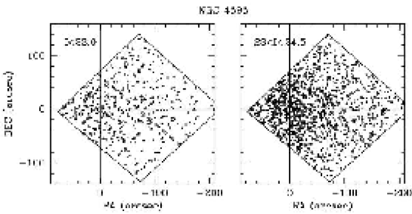
Figure 16: Left panel: Locations of the brightest globular clusters around NGC 4696. These objects follow the broad unimodal MDF shown in Fig. 7 above. The galaxy center is marked by the crosshairs and a $5^{\prime\prime}$ circle around the nucleus. The quadrangle, about $3\farcm 4$ on a side, marks the borders of the Multidrizzled ACS/WFC frame, and the image is oriented with North up and East to the left. The dashed lines show the dead space between the two WFC CCD detectors. Right panel: Spatial distribution for fainter globular clusters in NGC 4696, which follow a normal bimodal MDF. Both bright and faint clusters are concentrated to the galaxy center.

In addition, as far as we can tell, the luminous “unimodal” clusters do not have any different spatial distribution than the less luminous clusters. An example is shown in Figure 16, where the locations of the brightest clusters in NGC 4696 are plotted in comparison with a large sample of the fainter ones. No differences are evident; the brightest ones are found everywhere through the halo but with the same degree of central concentration as the others. More detailed tests of the radial profiles (shown in Figure 17) indicate no quantitative difference in the slope $\Delta{\rm log}\sigma_{cl}/\Delta{\rm log}r$. The other galaxies, though with smaller statistical samples to work with than NGC 4696, exhibit no different pattern. This evidence indicates that the broad spread of colors at the high-luminosity end is not associated in some way with a particular type of cluster formation (say) in the inner bulge region or the outer halo.

In summary, aside from a few objects with slightly more extended structures, the brightest clusters show no additional distinguishing features from the rest of the globular cluster population. We conclude that their color distribution must then correlate in some more direct way with cluster luminosity and (thus) mass.

5.5 Connections to dE Nuclei

Another special group of objects strongly resembling the globular clusters in luminosity, size, and (probably) age are the nuclei of dwarf elliptical galaxies. The massive cluster NGC 6715 forms the nucleus of the Sagittarius dwarf elliptical (Layden & Sarajedini, 2000), and the extended structure and multicomponent population within $\omega$ Centauri have raised suggestions that it might be the relic nucleus of a former dE satellite of the Milky Way (e.g. Majewski et al., 2000; McWilliam & Smecker-Hane, 2005). Similar ideas have been raised for M31-G1 (Meylan et al., 2001). Could the luminous cluster population be a collection of dE,N nuclei accreted long ago and stripped of their envelopes? This discussion can be traced back to early ideas by Zinnecker et al. (1988) and Freeman (1993) and has been explored in a variety of ways since. The sheer numbers of such objects do not appear to present an obstacle by themselves, since in normal hierarchical-merging galaxy formation models it takes thousands of dwarf-sized pregalactic clouds to eventually accumulate into one giant elliptical. If only a fraction of these happened to contain very massive globular-cluster-like nuclei, they could account for the few hundred that we see in our combined sample. Furthermore, extensive quantitative models have been developed to explore the possibility that many or most of the low-metallicity globular clusters in major galaxies might have been accreted from dwarf satellite galaxies (Côté et al., 2000). In this view, a bimodal MDF is not a required outcome, but rather a statistical result of the particular mass spectrum of accreted satellites, so a broad unimodal MDF is a definite possibility. (It is not at all clear, however, how this model can give rise to an MDF within one galaxy that is simultaneously bimodal at lower luminosities and yet unimodal at higher luminosities.)

Objects such as UCDs and the nuclei of nucleated-dwarf dE,N galaxies are quite hard to tell apart from traditional globular clusters if we have data in hand that consist only of luminosities, colors, and upper limits on their characteristic sizes. However, if we cannot individually identify clusters that were once dE,N nuclei, we can at least compare our BCG globular cluster population with the nuclei that are now in dE,N dwarfs. Fortunately, a comprehensive and homogeneous photometric study of dE,N nuclei from HST/WFPC2 imaging exists (Lotz et al., 2004) that can be used for this purpose.

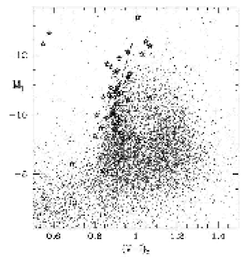
Figure 18: Composite color-magnitude diagram for the clusters in all eight of our BCGs, where our measured $(B-I)$ colors have been transformed to equivalent $(V-I)_{0}$. The large open stars show the locations of the nuclei of nucleated dwarf dE,N galaxies, from Lotz et al. (2004). The dashed line is explained in the text.

We show this comparison in Figure 18. Here, the data from all eight of our BCG fields are combined together, and overplotted with the photometry for the dE,N nuclei in the Virgo and Fornax groups, with data taken from the catalog of Lotz et al. (2004). To the Lotz et al. measurements we have added three more dE,N objects for which luminosities and colors are available: NGC 6715 in the Sagittarius dwarf (data from Harris 1996), and the nuclei of NGC 5206 (Caldwell & Bothun, 1987) and NGC 3115B (Durrell et al., 1996b). To normalize the colors of all these objects to the $(V-I)$ scale used by Lotz et al., we have converted our $(B-I)$ measurements and the other $(B-V)$ data in the literature through empirical relations shown in Figure 19, defined by the Milky Way globular clusters. The lines shown in the Figure are given by

$$(B-V)_{0}\,=\,0.96(V-I)_{0}-0.19,$$ (6)

$$(B-I)_{0}\,=\,1.96(V-I)_{0}-0.19.$$ (7)

Aside from a couple of very blue nuclei (interpreted as younger, more recently formed clumps; see Lotz et al. 2004), the nuclei define a moderately broad sequence over a luminosity range $M_{I}<-9$ similar to the traditional bright globular clusters. The very most luminous nuclei extend up to $M_{I}\sim-12.5$, as does the top end of the globular cluster population. However, the most striking feature of the dE,N sequence is that it lies entirely along the blue side of the globular cluster distribution; essentially none of them fall within the red-cluster population. We can think of no observational selection effect that would prevent slightly redder nuclei from being detected, and since the photometry is based on HST/WFPC2 images, the nuclei can be well separated from contamination by the surrounding dE envelopes. Lotz et al. note that the colors of the nuclei are consistently bluer than those of the dE galaxies they are embedded in, and thus by assumption should be either old and metal-poor, or (if they are actually the same metallicity as their host dE’s) much younger.

At a finer level of detail, the dE,N sequence is bluer by $\sim 0.05-0.1$ mag than the center of the blue-cluster sequence. It is not clear if this offset in color is significant: it may at least partly arise from transformation errors between one color index and another, or the combined zeropoint errors in the WFPC2 and ACS photometric data. Their location would, however, be consistent with the interpretation that most of the nuclei are old and metal-poor and thus acted as the first “seed” structures formed in their host dwarfs (see Lotz et al., 2004; Durrell et al., 1996a).

Regardless of how the dE,N nuclei are interpreted, it seems clear that many of the luminous globular clusters in our BCG sample have a different origin. Although dE,N nuclei could provide the source for many of the luminous blue clusters, most of the globular clusters at all luminosities are quite a bit redder than the nuclei. The simplest interpretation is most of them are not the relics of dE,N dwarfs that were accreted by the BCGs at some later time long after the major formation stage. An alternate, albeit more complex, interpretation would be that the dE,N dwarfs still remaining today (such as the Virgo and Fornax members used above) are preferentially more metal-poor and isolated than the ones accreted by the BCGs at earlier times. But we believe it is highly unlikely that dynamical processes could have selectively removed all of the hypothetical dE,N galaxies with intermediate- or high-metallicity nuclei while leaving behind only a few with metal-poor ones.

Another interpretation that has been offered for the UCDs and objects like NGC7252-W3 is that they are merged products of several young massive star clusters that formed from cluster complexes in major starbursts (Fellhauer & Kroupa, 2002). This mechanism also appears unlikely to explain the luminous population we see: as discussed by Fellhauer & Kroupa (2002), such merger products would have very large effective radii unlike globular clusters, and most of them would be expected to be metal-rich if they formed during the late major starbursts.

Our general conclusion from these comparisons is that some of the luminous blue clusters could well be accreted dE,N nuclei, but that the red cluster population is more likely to have a different origin as normal globular clusters.

6 Bimodality Model Fits: A Mass-Metallicity Relation

To test in more detail what happens to the two obvious “modes” (blue and red) as a function of cluster luminosity, we carried out a series of tests where the MDF is modelled, as before, by a combination of two Gaussian distributions. We allowed both the dispersion and mean color to be solved for. In each galaxy we grouped the MDF into magnitude bins containing 200 objects per bin, so that each bin would have similar statistical uncertainties.

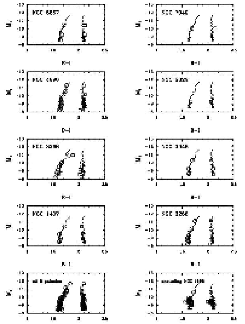
Figure 20: Mean colors for the individual GCSs in the eight BCGs. In each panel, the clusters are subdivided into magnitude bins of 200 objects per bin. The KMM mixture modelling code is used to fit two Gaussians to the color distribution in each bin, with resulting mean colors shown by the open circles (metal-poor clusters) and open squares (metal-rich clusters) in each panel. The graph at lower left shows the composite population for all eight galaxies; the jagged line through its set of points is reproduced in all the other panels for comparison. The graph at lower right shows the mean lines for seven galaxies excluding NGC 4696.

In Section 3 above, we described the fits to the composite 8-galaxy sample. Here, we show the results for the individual galaxies, displayed in Figure 20. The lower left panel is our previous composite fit for all eight galaxies combined and shows the trend of mean color with absolute magnitude $M_{I}$ (traced by the two jagged lines that pass through the mean points). These lines are reproduced in each of the other panels for comparison.

Of the principal results emerging from these fits, we note first that since each mean point is independent of the others, the very small offsets between the individual bin points and the mean lines in Fig. 20 demonstrate that all the MDFs exhibit bimodality with a high degree of reliability, and with nearly identical patterns in the different galaxies.

Secondly, the mean color of the red mode shows no significant change with luminosity. That is, there appears to be no mass-metallicity trend for the more enriched clusters that are the most likely to have formed in the major series of starbursts that built the main body of the parent galaxy.

Thirdly, the KMM solutions for the blue-cluster sequence suggest a correlation between color and luminosity beginning at about $M_{I}\simeq-9.5$. The effect is most noticeable for the galaxies with the largest observed cluster populations (namely NGC 1407, 3258, 3268, 4696) that carry the most weight in the definition of the mean lines in Fig. 20. The other four (NGC 3348, 5322, 5557, 7049) do not disagree with the same trend, but they do not carry enough statistical weight by themselves to say whether the same trend exists within them individually. Although this correlation may at least partly be bound up with our lingering concerns about photometric calibration and the small differences between psf-based and aperture-based photometry, we find that it is present in all our galaxies (see again Fig. 10b) regardless of which type of data we use, either aperture or PSF-fitting.

Since $(B-I)$ depends linearly on [Fe/H], and absolute magnitude varies logarithmically with luminosity (hence mass), the color/magnitude trend turns directly into a simple power-law scaling of heavy-element abundance $Z$ with cluster mass $M$. The result for the combined sample is displayed in Figure 21, where we have adopted as before a mean mass-to-light ratio $(M/L)_{V}\simeq 3$. The ratio $(M/L)$ is difficult to measure accurately and is likely to differ somewhat between clusters (e.g. Meylan et al., 1995; McLaughlin, 2000; Baumgardt et al., 2003; Pasquali et al., 2004; Martini & Ho, 2004) but we assume it to be roughly invariant with luminosity. For the blue cluster population, we then find

$${Z\over Z_{\odot}}(GC)\,\simeq\,10^{-5}({M\over M_{\odot}})^{0.55}$$ (8)

for masses higher than about $6\times 10^{5}M_{\odot}$ (equivalent to $M_{I}\simeq-9.5$, which is about a magnitude brighter than the GCLF turnover).

The dE,N nuclei discussed above follow a very similar trend of mean color with luminosity, again starting at a similar luminosity level $M_{I}\simeq 10$. This correlation is shown as the dashed line in Fig. 18, which corresponds to a metallicity scaling $Z\sim M^{0.55}$. This comparison reinforces the idea that the nuclei are structurally similar entities to the bright, low-metallicity globular clusters.

Although too much weight should not be placed on the datapoints at lower luminosities, where the photometry becomes more uncertain and more affected by field contamination, it does not seem likely that the same power-law scaling continues downward to lower masses. The main reason for this suggestion is that on external grounds we expect the “bottom end” in metallicity for the metal-poor clusters to be at a mean [Fe/H] $\simeq-1.6$, where we find the blue mode for clusters in the Milky Way and in a wide range of dwarf ellipticals (Harris & Harris, 2001; Burgarella et al., 2001; Lotz et al., 2004; Woodley et al., 2005), and near where the low-luminosity end of our BCG sequence lies.

7 Metallicity Dispersions

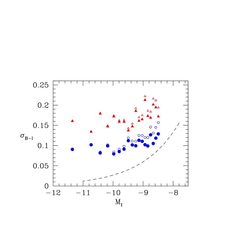
Figure 22: Measured dispersions of the blue and red cluster MDFs. Here $\sigma_{B-I}$, the rms dispersion of each mode as determined from the double-Gaussian fits described in the text, is plotted versus $I$ magnitude: small open circles are the metal-poor clusters, small open triangles the metal-rich clusters. The dashed line shows the average photometric measurement uncertainty $\sigma_{phot}$; when this is subtracted in quadrature from $\sigma_{B-I}$, the resulting estimate of the intrinsic metallicity dispersion of each mode is shown with the larger solid symbols.

The intrinsic dispersions of the red and blue modes are well resolved in our data, and emerge more clearly here than in most previous studies. They can therefore be used to estimate the internal range of abundances of each type of cluster. The internal dispersions are noticeably different in the two modes, averaging $\langle\sigma_{B-I}\rangle=0.099\pm 0.007$ for the blue mode and $0.166\pm 0.014$ for the red mode (Table 3). In Figure 22, we show $\sigma(B-I)$ as deduced directly from the KMM two-Gaussian model fits, plotted as a function of luminosity $M_{I}$. The directly observed dispersions grow progressively larger for $M_{I}>-9.5$, but this is at least partly a result of the increasing field contamination as well as the photometric measurement uncertainty (shown as the dashed line in the figure; since the photometric limits in $M_{I}$ are very similar from one galaxy to the next, we show only the mean line). A better estimate of the residual intrinsic dispersion is $\sigma_{0}=(\sigma_{B-I}^{2}-\sigma_{phot}^{2})^{1/2}$, where the main effect of at least the photometric scatter is removed. The $\sigma_{0}$ values, also plotted in Fig. 22, suggest that the intrinsic $(B-I)$ spread of each mode is near $\sigma_{0}(blue)\simeq 0.10$ and $\sigma_{0}(red)\simeq 0.16$. These translate to $\sigma$[Fe/H] = 0.27 dex for the metal-poor clusters and 0.43 dex for the metal-rich ones, assuming that the linear conversion from color to metallicity is valid.

8 Radial Color Distributions

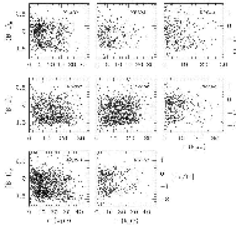
Figure 23: $(B-I)_{0}$ versus radius for each of the BCG fields. Here only the brighter objects are selected as described in the text, to minimize field contamination from faint and predominantly blue objects. Color is converted to metallicity [Fe/H] following Eqn. (5).

Figure 23 shows the dereddened cluster colors versus projected galactocentric distance $r$; for convenience of comparison, we convert the radial distances $r$ to kiloparsecs, and also show the [Fe/H] scale on the right-hand edge of each plot. We find little or no significant trend of color with radius (thus by assumption metallicity) within either population. Any systematic color gradient with galactocentric distance must then be the straightforward result of a changing ratio of blue-to-red relative numbers with radius. This latter effect was shown to exist for the GCSs in NGC 4472 by Geisler et al. (1996) and has been found in other systems since (e.g. Harris et al., 1998; Dirsch et al., 2003; Rhode & Zepf, 2004).

As a simple indicator of the trend, in Table 5, we show the progressive change in the ratio $N(red)/N(total)$ with projected galactocentric radius for all eight systems. These are listed in four radial bins, $0-5$ kpc, $5-10$ kpc, $10-20$ kpc, and $>20$ kpc. For each bin, we list the total number of clusters, then the ratio $N(red)/N(total)$. To minimize field contamination when counting probable clusters, we simply exclude objects bluer than $(B-I)_{0}=1.3$, redder than 2.3, or fainter than $M_{I}=-9.0$, and we define $(B-I)_{0}=1.8$ as the dividing line between the two populations. The trends are plotted in Figure 24.

All the GCSs show evidence for population gradients. The largest part of the effect comes from within $R_{gc}=5$ kpc, where the red clusters are always more dominant, as would be expected if they belong to later formation epochs when enriched gas had already concentrated deeper into the potential well of the major galaxy. In all our BCGs, the red clusters make up more than half the population within 5 kpc, and can make up as much as 80% in the most extreme case. Outward of 5 kpc, however, little or no gradient shows up for any of the systems. In a later paper, we will explore the radial distributions and total populations in more detail.

The total numbers of red vs. blue clusters that we observe in our target systems differ quite a lot from one galaxy to the next. The ratio $N(blue)/N(red)$ ranges from $\sim 0.6$ in NGC 1407 up to $\sim 1.5$ in NGC 3258. But at least part of this range may be due to the fact that the galaxies are at different distances, so that we do not sample the same true range in galactocentric radius $r_{gc}$ in each one. For the closer systems we are seeing only the inner and middle regions of the halo, and if the red clusters are more centrally concentrated we will see proportionally more of them than in an intrinsically similar but more distant galaxy. In Table 5, we show the average $f(red)$ in the last line for the various radial bins. The values of $f(red)$ for the individual galaxies have internal uncertainties that are only scarcely larger than the rms scatter among the galaxies, indicating that the differences are not highly significant. We note, however, that if the dominant formation mechanism for these BCGs is hierarchical merging, then in a rough sense we would expect more galaxy-to-galaxy variance among the red-cluster population, since they arise from a small number of major mergers in the late stages of formation and thus are subject to potentially large stochastic variations (Beasley et al., 2003). By contrast, the blue clusters are formed from a large number of small formation events within the pregalactic dwarf population and thus their relative numbers should be more consistent from one BCG to the next.

9 Discussion

The underlying cause for the bimodal nature of the globular cluster MDF is still something of a mystery. Ideas have been suggested involving preferentially early or quick formation of globular clusters in the very first stages of galaxy formation, when few stars had yet formed and the gas was in the form of numerous very low-metallicity, dwarf-sized clouds (Harris & Harris, 2002; Beasley et al., 2002). This first round of formation would have produced many low-metallicity clusters, but because it was happening in many relatively small potential wells, much of the remaining gas could have been ejected by stellar winds and supernovae, preventing it from being incorporated into stars till much later. However, these ideas have not yet developed into a full quantitative picture. One important concern is that recent simulations (e.g., Mac Low & Ferrara, 1999; Fragile et al., 2004) suggest dwarfs with more than $\sim 10^{9}M_{\odot}$ of gas would have suffered relatively little mass loss for plausible supernova rates. Thus if early cluster formation went on in potential wells at least this massive, there appear to be no reason why clusters could not have continued to form into intermediate and high metallicity regimes.

In addition, it seems to be important that the same bimodality phenomenon now regarded to be normal for globular clusters does not show up in the halo and bulge field stars of E galaxies, the MDFs for which are broad, unimodal, and contain relatively few metal-poor stars (Harris & Harris, 2002). An alternate way to state this dichotomy is that the specific frequency of the stellar population, defined as the number of clusters per unit galaxy light within a given metallicity range, needs to be typically at least $\sim 5$ times higher for the metal-poor regime ([Fe/H] $<-1$) than for the metal-rich regime [Fe/H] $>-1$ (Harris, 2001, 2002; Forte et al., 2005). At face value, the evidence suggests that large galaxies were very much more efficient at producing high-mass star clusters at early times when the gas fraction was extremely high and the metallicity extremely low, than they were later on during the major field-star formation stages.

Conversely, it might be selective destruction rather than formation mechanisms that is responsible for the specific frequency difference. Perhaps the low-metallicity star clusters that form in dwarf galaxies are more likely to survive destruction during their infancy than their high-metallicity counterparts in larger galaxies (e.g. Whitmore, 2005). This effect might be especially relevant for clusters that form at the centers of dwarf galaxies (e.g. Lotz et al., 2004), where the tidal stress is low and where they might be able to build up to very large masses. The fundamental characteristic of bimodality (the rather distinct gap between metal-poor and metal-rich subpopulations), however, eludes satisfactory explanation as yet.

As we have done in the preceding discussion, we adopt here the “default” view that the cluster colors are indicators of heavy-element abundance rather than age. For clusters older than $\sim 5$ Gy, broadband optical colors are sensitive primarily to metallicity and only secondarily to mean age. For comparison, it is worth noting that the metal-poor clusters in the Milky Way show no systematic differences in age larger than $\sim 1$ Gy (e.g. Rosenberg et al., 1999), and the metal-rich clusters may be only $\sim 2$ Gy younger in the mean. However, the red-cluster population clearly exhibits a much larger internal dispersion in the giant ellipticals than in the Milky Way, perhaps reflecting the series of major mergers and starbursts that the galaxy was built from in a hierarchical-merging scenario (e.g., Beasley et al., 2002, 2003). Under these conditions, a cluster-to-cluster age range of a few Gy would be more likely a priori. Globular cluster age ranges at this level within selected giant E galaxies have recently been claimed through spectral-index analysis, although the majority of the clusters still appear to be 10 Gy old or more (e.g., Beasley et al., 2000; Forbes et al., 2001; Jordan et al., 2002; Puzia, 2003; Larsen et al., 2003; Hempel et al., 2003; Peng et al., 2004). Even so, an age scatter of just a few Gy would generate a color spread of 0.1 mag or less, not enough to match the intrinsic scatter in color that we find in either the blue or red modes.

An excellent recent overview on globular cluster formation models is given by Kravtsov & Gnedin (2005). Three major contributors to the GCS populations within large galaxies conventionally include (a) early in situ formation (Harris & Pudritz, 1994; Forbes et al., 1997), (b) major mergers that are sufficiently gas-rich to form large numbers of new clusters (Whitmore et al., 1999; Zepf et al., 1999, among many others), and (c) ongoing accretion of gas-free satellites (Côté et al., 2000). In certain circumstances, it may be possible to isolate one or the other of these as the dominant mechanism. For example, “field” elliptical galaxies with low GCS specific frequencies $S_{N}<2$ and a wide mixture of cluster ages are excellent candidates to have formed from a small number of major mergers of disk galaxies (Harris, 2001). In the Milky Way, late mergers are not important, but accretion of small, low-metallicity satellites may have been responsible for building much of the halo (Côté et al., 2000).

For the giant BCGs, we are more likely to be looking at the combined result of all three processes in their full complexity, making it more difficult to separate out their effects. For this reason, in the following discussion we adopt the viewpoint of a hierarchical-merging scheme arising from standard CDM cosmologies. In this framework we essentially subsume all three individual processes into one (albeit complex) sequence: at very early times, many small clouds within a large dark-matter potential well merge progressively and rapidly into a “seed” giant elliptical; later on, a few major mergers may take place; then finally, a low-level process of satellite accretion continues to the present time.

Within this hierarchical-merging context, the blue, metal-poor clusters are regarded to have formed first within the original population of pregalactic gas clouds (the so-called “quiescent mode”, before truly big mergers were occurring). A similar view has frequently been argued on other grounds (Harris & Pudritz, 1994; Burgarella et al., 2001; Harris & Harris, 2002; Beasley et al., 2002; Kravtsov & Gnedin, 2005). The red, metal-rich clusters then formed during the later mergers that built the main body of a giant galaxy, the latter stages of which may still be continuing today. Some major pieces of observational evidence which are strongly consistent with this general view are:

• The MDF of the field stars matches up well with the MDF of the metal-rich globular clusters (Harris & Harris, 2002; Harris, 2002; Forte et al., 2005), as expected if they formed in lockstep during the sequence of starbursts generated by mergers.

• In most giant ellipticals including BCGs, the metal-rich clusters form a more centrally concentrated radial distribution around their parent galaxy than do the metal-poor clusters. In turn, the red-cluster distribution is usually found to match up well with the galaxy halo light profile as a whole, again consistent with their contemporaneous formation.

• The globular clusters in dwarf elliptical galaxies are almost entirely of low metallicity, consistent with their having evolved directly from protogalactic gas clouds that experienced few or no mergers (Durrell et al., 1996a; Lotz et al., 2004).

• The mean colors of both the metal-rich and metal-poor modes increase weakly with parent galaxy luminosity, indicating that the total size of its potential well influenced the degree of heavy-element enrichment from the start (e.g. Strader et al., 2004; Lotz et al., 2004).

Our new data provide additional constraints on the enrichment history of the globular clusters. If the formal double-Gaussian fits (Fig. 21) are on the right track, then we have a series of new observational features to deal with:

• The formation of the low-metallicity clusters (presumably the oldest ones) must apparently allow for higher metallicity at higher cluster mass, at least in some major galaxies such as BCGs;

• Contrarily, for the red (metal-rich) cluster sequence, there is no trend in mean metallicity with luminosity;

• At all luminosities, the cluster-to-cluster spread in heavy-element abundance $\sigma_{logZ}$ is quite significant, and is larger and more variable from galaxy to galaxy for the red clusters than for the blue ones.

A plausible interpretation for the first item seems to us to be connected with an idea previously stated in the literature, that on the average, higher-mass clusters require more massive reservoirs of gas out of which to form. The typical observational scaling ratio is that the host gas cloud is $\sim 10^{3}$ times more massive than any single average star cluster that forms within it (Harris & Pudritz, 1994). The smaller globular clusters – those with masses $<10^{5}M_{\odot}$ – could then typically have formed within pregalactic clouds containing only $\sim 10^{7}-10^{8}M_{\odot}$ of gas, while the very most massive globular clusters known (those with $M>10^{7}M_{\odot}$) would have required reservoirs of gas as high as $10^{9}-10^{10}M_{\odot}$. The potential wells within these bigger clouds would be massive enough to hold on to their gas during the first violent rounds of star formation and thus partially self-enrich shortly before the first massive star clusters appeared, allowing them to build up to higher metallicity. At the same time, these most massive host dwarfs could have escaped the “gap” or interruption at intermediate cluster metallicities that affected the lower-mass clusters almost universally. Clearly, however, some crucial elements of this descriptive story are still missing.

Further evidence that the metallicities of the massive clusters are intimately tied to their parent cloud masses may come from two other scaling relations. For dwarf galaxies, the mean metallicity is observed to vary with total stellar mass $M_{\star}$ as (Dekel & Woo, 2003)

$${Z\over Z_{\odot}}(dwarf)\,\simeq\,4\times 10^{-5}M_{\star}^{0.40}$$ (9)

where $M_{\star}$ is in Solar units. However, it is the dark matter in the dwarf that dominates its potential well, and an observationally based scaling of the ratio of dark matter to stellar mass is (Persic et al., 1996)

$${M_{DM}\over M_{\star}}\,\simeq\,34.7M_{\star,7}^{-0.29}$$ (10)

where here $M_{\star,7}$ is in units of $10^{7}M_{\odot}$. Combining Eqs. (9) and (10), we obtain

$${Z\over Z_{\odot}}(dwarf)\,=\,3.9\times 10^{-7}M_{DM}^{0.56}.$$ (11)

This latter relation has a similar slope to the one suggested above for the metal-poor clusters. At this stage, we view this comparison as little more than suggestive. However, the implication for our purposes is that the most massive star clusters can end up with heavy-element abundances determined directly by the dark-matter potential wells of the pregalactic clouds that they formed in, since $M_{DM}$ would determine the metallicity of the ambient gas from which they formed. Notably, Lotz et al. (2004) find, for the globular cluster populations in dwarf E galaxies, that the mean metallicity $Z(GC)$ of the clusters scales with the luminosity of the host galaxy as $Z(GC)\sim L_{dE}^{0.2}$. This is a slightly shallower trend than the ones for the dwarfs themselves, but one which also argues that the enrichment of a given cluster increases with the mass of its host environment.

As mentioned above, current numerical simulations (see, e.g., the extensive discussions of Mac Low & Ferrara, 1999; Fragile et al., 2004) indicate that dwarfs with gas masses less than $10^{8}M_{\odot}$ have heavy-element ejection efficiencies approaching 100% for a range of plausible supernova rates and distributions. However, model dwarfs with masses above $10^{9}M_{\odot}$ successfully retain their heavy elements except under extremely high starburst conditions. It is the dwarfs in this upper range that should be capable of building globular clusters with masses well above $10^{6}M_{\odot}$.

The cluster-to-cluster scatter of metallicity at a given mass could well have been generated by the random nature of the starbursts within their host dwarfs, since the metal ejection efficiency depends on the detailed locations of the individual supernovae as well as their ignition rates (cf. the references cited above).

Lastly, within the same hierarchical-merging picture, why would the metal-richer cluster sequence not show the same kind of mass/metallicity relation as the blue clusters? We suggest that the explanation may lie in the relative epoch of their formation. These objects would have formed in the bigger, later mergers and starbursts that built the main stellar population of the galaxy. Each of these major bursts could have assembled gas clouds (GMCs and GMC complexes) of a very wide range of sizes and masses, within which star clusters of a similarly broad range could form, such as we see happening in contemporary mergers (Whitmore et al., 1999; Zhang et al., 2001; Wilson et al., 2003). What distinguishes these later stages from the earlier initial stage is that the large-scale potential well of the new BCG has now formed, and gas cooling times are shorter at the higher metallicities, allowing newly enriched gas to be retained throughout the body of the galaxy. The combination of these factors may then have allowed this second major group of globular clusters to form along with the field stars in a common MDF that is extremely broad (Harris & Harris, 2002), and with no net mass-metallicity relation.

As mentioned earlier, we believe that another important characteristic of the metal-richer population is that both its mean metallicity and internal metallicity dispersion are less uniform from one galaxy to the next than those of the metal-poor population. These can be seen from the plots of $\langle B-I\rangle$ and $\sigma(B-I)$ (Fig 10), where the red population displays variations twice as large as for the blue. We suggest from these comparisons that the red population differs internally in both metallicity and age to a degree larger than in the bluer mode. As noted above, such differences would be expected if they were primarily formed in the last few major mergers and thus subject to larger stochastic variations.

In this general scheme, the metal-richer cluster formation mode can be thought of as the “normal” one in the sense that these clusters match well with the MDF of the halo stars in the galaxy. It is the metal-poor ones that are anomalous because of their very high specific frequency. Further quantitative models tuned specifically to following globular cluster formation will need to be pursued in order to understand exactly what was special about that first, remarkably efficient mode.

10 Summary

We present new HST ACS/WFC photometry in $(I,B-I)$ for globular cluster systems in eight giant ellipticals, all of which are centrally dominant objects (BCGs) in clusters of galaxies. In all cases the photometry reaches to limits at or beyond the turnover point in the globular cluster luminosity function, and clearly resolves the internal spread in colors of the clusters.

All of the $(B-I)$ distributions are clearly bimodal, strongly supporting the view built up in recent years that globular clusters in major galaxies come in two distinctive types: metal-rich and metal-poor. With the use of a metallicity-sensitive color index and high-quality photometry, the structure of the metallicity distribution function (MDF) is more clearly revealed here than in all but the best previous studies.

We find that in several of our target galaxies, the blue and red modes effectively overlap or merge at high luminosity, specifically in the range $M_{I}<-10.5$ (corresponding to cluster masses higher than $10^{6}M_{\odot}$). At these high-luminosity, high-mass levels, extremely metal-poor clusters become much rarer, and intermediate-metallicity clusters much more common than at the lower levels where bimodality is much more sharply evident. This effect is a result of a correlation between luminosity and color that sets in within the metal-poor cluster sequence, shifting it progressively redward towards higher luminosity and causing it to overlap with the red cluster sequence. Furthermore, the larger the total measured cluster population contained in the galaxy, the more clearly this feature emerges. Comparisons with other published studies suggest to us that this phenomenon may be particularly associated with these giant BCGs. A compelling interpretation is not yet obvious, but if we make the plausible assumption that more massive clusters on average must form within proportionally larger parent gas clouds, then our data suggest to us that the most massive globular clusters formed within parent clouds that were massive enough in turn to hold on to more of their gas and reach higher levels of pre-enrichment. The recent literature suggests that the enrichment effect will set in for dwarfs of gas masses $10^{9}M_{\odot}$ or more, large enough to produce globular cluster masses of $>10^{6}M_{\odot}$.

We find that both the intrinsic color dispersion and mean color of the red-cluster population differ more from galaxy to galaxy than the blue-cluster population. We do not see any pattern to these differences; they are not obviously correlated with galaxy luminosity, total measured cluster population, blue-to-red relative numbers of clusters, or the richness of the galaxy cluster they are in. Within the context of standard hierarchical-merging galaxy formation models, we suggest that these very noticeable differences in the red-cluster population may be due to stochastic variations in the last few major mergers that built the galaxy. By contrast, the blue-cluster population was built through a large number of smaller-scale events in the pregalactic cloud population and thus is more nearly universal in form.

Finally, we find clear evidence for population gradients in all the BCGs in our sample. Within $\sim 5$ kpc of galaxy center, every galaxy contains a distinctly higher proportion of red, metal-rich clusters. Beyond 10 kpc, however, the residual color gradient becomes much smaller.

The two major and long-standing issues that our data reinforce are (1) the basic bimodality property of the globular cluster MDF, which still lacks a convincing physical explanation, and (2) the large numbers of metal-poor clusters relative to the small numbers of metal-poor field halo stars that these giant galaxies possess. If the hierarchical-merging models are essentially correct, in their earliest star-forming era the pregalactic clouds went through a short period of producing massive star clusters at high efficiency. The later production of the redder, metal-richer clusters through major mergers and starbursts can now be thought of as a familiar and reasonably well understood process, since modern-day gas-rich mergers are seen producing these kinds of clusters actively. It is the earlier, pregalactic era that produced roughly the same total number of massive clusters as all the later epochs combined, and that is still poorly understood.

In later papers, we will present further MDF data for five more BCGs, and discuss their globular cluster luminosity distributions, specific frequencies, and spatial structures.

Table 1: Brightest Cluster Galaxies Imaged with the ACS

NGC	Cluster	Redshift	$M_{V}^{T}$	$E(B-I)$	$(m-M)_{I}$	$B$ Exposures	$I$ Exposures
	or Group	(km s-1)			($M_{I}<-8.4$)	(sec)	(sec)
1407	Eridanus	1627	$-22.35$	0.16	31.96	$2\times 750$	$2\times 340$
5322	CfA 122	1916	$-22.01$	0.03	32.22	$3\times 1130$	$2\times 410$
7049	N7049	1977	$-21.76$	0.12	32.36	$6\times 580$	$3\times 400$
3348	CfA 69	2837	$-22.13$	0.17	33.18	$6\times 1200$	$4\times 530$
3258	Antlia	3129	$-21.87$	0.20	33.23	$4\times 1340$	$4\times 570$
3268	Antlia	3084	$-21.96$	0.24	33.27	$4\times 1340$	$4\times 570$
4696	Cen30	2926	$-23.31$	0.23	33.29	$4\times 1360$	$4\times 580$
5557	CfA 141	3213	$-22.32$	0.01	33.31	$2\times 1280,2\times 1350$	$4\times 600$

Table 2: Measured Populations and Field Contamination Levels

NGC	$N_{c}$	$N_{f}$	$N_{f}/N_{c}$
1407	402	2.5	0.01
5322	126	2.5	0.02
7049	196	22	0.11
3348	374	15	0.04
3258	885	31	0.04
3268	780	29	0.04
4696	1587	116	0.07
5557	357	18	0.05

Table 3: Bimodal Fitting Parameters

NGC	$N_{b}/N_{r}$	$\langle B-I\rangle_{0}$	$\sigma_{B-I}$	$\langle B-I\rangle_{0}$	$\sigma_{B-I}$	$\Delta\langle B-I\rangle$
		(blue)	(blue)	(red)	(red)	(red$-$blue)
1407	0.60	$1.63\pm 0.02$	$0.12\pm 0.02$	$2.07\pm 0.01$	$0.13\pm 0.01$	$0.44\pm 0.03$
5322	1.10	$1.67\pm 0.01$	$0.07\pm 0.01$	$2.01\pm 0.02$	$0.09\pm 0.01$	$0.46\pm 0.02$
7049	1.25	$1.67\pm 0.04$	$0.12\pm 0.02$	$2.14\pm 0.06$	$0.21\pm 0.14$	$0.47\pm 0.07$
3348	0.70	$1.60\pm 0.01$	$0.07\pm 0.01$	$2.07\pm 0.02$	$0.17\pm 0.02$	$0.47\pm 0.02$
3258	1.49	$1.61\pm 0.01$	$0.10\pm 0.01$	$2.01\pm 0.03$	$0.20\pm 0.04$	$0.40\pm 0.03$
3268	1.10	$1.61\pm 0.01$	$0.10\pm 0.01$	$2.01\pm 0.03$	$0.20\pm 0.04$	$0.40\pm 0.03$
4696	1.31	$1.67\pm 0.01$	$0.11\pm 0.01$	$2.09\pm 0.01$	$0.16\pm 0.01$	$0.42\pm 0.02$
5557	0.91	$1.66\pm 0.02$	$0.10\pm 0.01$	$2.10\pm 0.02$	$0.17\pm 0.03$	$0.44\pm 0.03$
BCG Mean	1.06	1.64 (0.03)	0.10 (0.02)	2.06 (0.05)	0.17 (0.04)	0.44 (0.03)
Milky Way	2.34	$1.57\pm 0.02$	$0.13\pm 0.02$	$1.95\pm 0.02$	$0.06\pm 0.02$	$0.38\pm 0.03$

Table 4: Gaussian Fits in Luminosity Bins for Individual Galaxies

NGC	$M_{I}=(-13.5,-10.5)$	$N$	$M_{I}=(-9.8,-9.5)$	$N$	$M_{I}=(-10.5,-9.0)$	$N$
1407	0.128	79	$6.2\times 10^{-7}$	85	$3.0\times 10^{-17}$	401
5322	0.12	13	–	–	$1.1\times 10^{-7}$	102
7049	0.161	45	0.016	39	$2.3\times 10^{-6}$	155
3348	0.238	66	$1.8\times 10^{-6}$	67	$1.6\times 10^{-11}$	319
3258	0.038	167	$5.7\times 10^{-9}$	165	$3.6\times 10^{-19}$	735
3268	–	161	$9.5\times 10^{-6}$	136	$4.2\times 10^{-15}$	632
4696	0.0015	342	$1.3\times 10^{-9}$	231	$2.9\times 10^{-31}$	1260
5557	0.0024	67	$0.016$	69	$1.6\times 10^{-10}$	304

Table 5: Red Cluster Population Ratios Versus Galactocentric Distance

NGC	$0-5$	$f(red)$	$5-10$	$f(red)$	$10-20$	$f(red)$	$>20$	$f(red)$
	kpc		kpc		kpc		kpc
1407	173	$0.79\pm 0.09$	163	$0.62\pm 0.08$	130	$0.62\pm 0.09$	3	$-$
5322	63	$0.68\pm 0.14$	45	$0.49\pm 0.13$	18	$0.50\pm 0.20$	0	$-$
7049	75	$0.69\pm 0.13$	82	$0.61\pm 0.11$	62	$0.45\pm 0.10$	7	$-$
3348	145	$0.69\pm 0.09$	116	$0.61\pm 0.09$	78	$0.63\pm 0.12$	30	$0.53\pm 0.17$
3258	125	$0.61\pm 0.09$	224	$0.42\pm 0.05$	418	$0.46\pm 0.04$	110	$0.46\pm 0.08$
3268	96	$0.57\pm 0.10$	196	$0.53\pm 0.06$	400	$0.51\pm 0.04$	84	$0.46\pm 0.09$
4696	156	$0.55\pm 0.07$	386	$0.48\pm 0.04$	580	$0.44\pm 0.03$	555	$0.41\pm 0.03$
5557	76	$0.75\pm 0.13$	107	$0.58\pm 0.09$	109	$0.59\pm 0.09$	54	$0.59\pm 0.13$
Mean		$0.67\pm 0.03$		$0.54\pm 0.03$		$0.53\pm 0.03$		$0.49\pm 0.03$

Figure 1: Distribution of observed half-light radii $r_{h}$ (in parsecs) for the Milky Way globular clusters, with data from Harris (1996). For the ACS images used in this study, the stellar point spread function (PSF) has a typical HWHM of 1.1 pixels, which is equivalent to 8.3 pc for a galaxy at a distance of 30 Mpc, as shown by the dashed line.

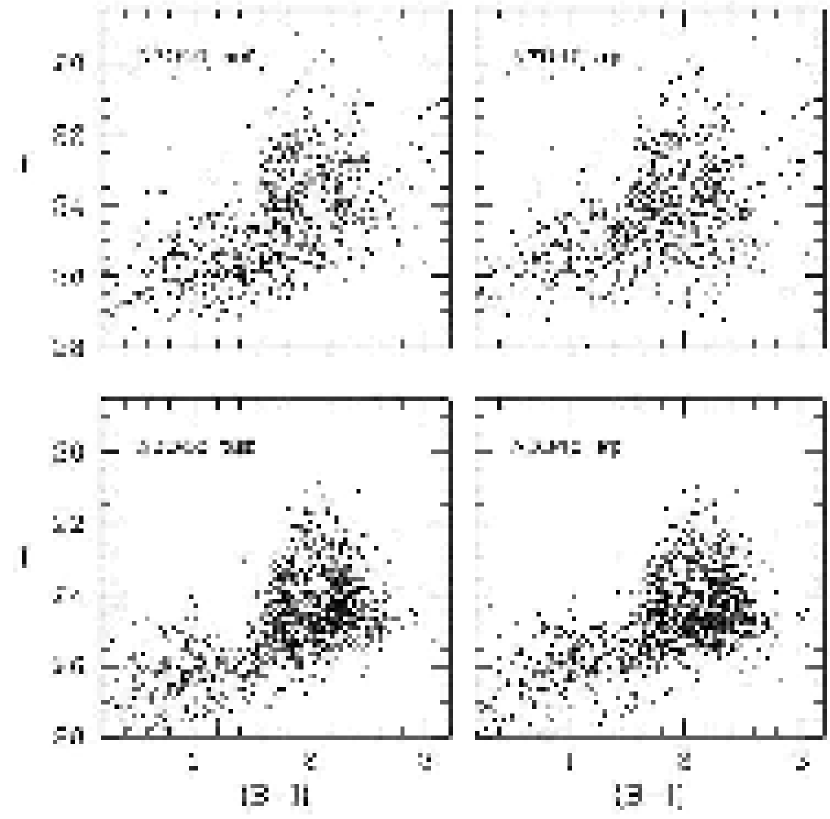
Figure 4: Color-magnitude plots for the cluster populations around NGC 7049 (top) and NGC 3348 (bottom).

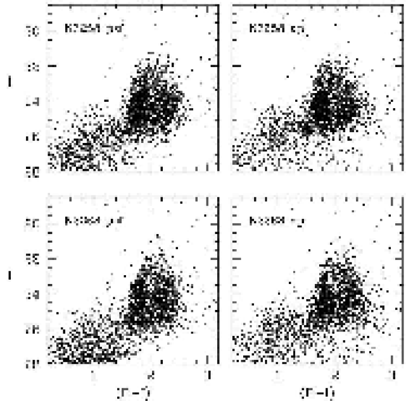
Figure 5: Color-magnitude plots for the cluster populations around NGC 3258 (top) and NGC 3268 (bottom).

Figure 7: Intrinsic color $(B-I)_{0}$ versus [Fe/H] for Milky Way globular clusters, taken from the 2003 edition of the Harris (1996) catalog. Clusters with lower reddenings ($E_{B-V}<0.4$) are plotted as large solid symbols, and ones with $0.4<E_{B-V}<1.0$ as small open symbols. The two dashed lines show the two linear least-squares solutions ([Fe/H] vs. $(B-I)_{0}$, or $(B-I)_{0}$ vs. [Fe/H]); the solid line is the adopted conversion as given in the text.

Figure 8: Upper panel: Results of the KMM model fits to the combined color distribution for all eight BCGs, subdivided into narrow luminosity bins. Here, $p$ is the probability that the color distribution within each bin can be represented by a single (unimodal) Gaussian; the logarithm of $p$ is plotted against the mean luminosity of the objects in the bin, $\langle M_{I}\rangle$. The luminosity intervals are defined so that 200 objects are in each bin. Lower panel: Solid line shows the fraction of clusters in the blue mode, plotted as a function of luminosity bin (ordinate on left side). The dashed line shows the difference $\langle B-I\rangle$(red) $-\langle B-I\rangle$(blue) between the peak colors of the two modes (ordinate on right side).

Figure 17: Spatial distribution of the globular cluster system in NGC 4696. The number of measured objects per unit area in the NGC 4696 ACS field is plotted against projected galactocentric distance. Open triangles show the bright clusters $(I<23)$, while solid symbols are fainter ones $(23<I<24.5)$. For these relatively bright magnitude intervals, completeness corrections and field contamination are negligible (see text).

Figure 19: Intrinsic colors for globular clusters in the Milky Way, with catalog data from Harris (1996). The left panel shows $(B-V)_{0}$ versus $(V-I)_{0}$, and the right panel $(B-I)_{0}$ versus $(V-I)_{0}$. Equations for the fitted lines are given in the text.

Figure 21: Mean intrinsic colors of the globular cluster populations as a function of luminosity, from the combined sample of eight BCGs. Metal-rich clusters are the solid symbols and metal-poor ones the open symbols. Each dot represents the mean of 200 objects; the uncertainty of each mean is similar to the size of the symbol. For the metal-rich clusters, the mean color is constant with luminosity at $\langle B-I\rangle_{0}=2.08$, equivalent to log $(Z/Z_{\odot})\simeq-0.21$. For the metal-poor clusters, objects brighter than $M_{I}=-9.5$ follow a scaling with mass given by log $(Z/Z_{\odot})=-5.0+0.55$ log $(M/M_{\odot})$ (shown by the sloped line).

Figure 24: Ratio of red clusters to total number of clusters, with data taken from Table 3. A typical error bar for the datapoints is shown at upper right. Open circles: NGC 1407. Open triangles: NGC 3258. Crosses: NGC 3268. Open pentagons: NGC 3348. Open stars: NGC 4696. Solid circles: NGC 5322 (lower) and NGC 5557 (upper). Solid triangles: NGC 7049.

References

- Ashman et al. (1994) Ashman, K.A., Bird, C.M., & Zepf, S.E. 1994, AJ, 108, 2348
- Baum (1955) Baum, W.A. 1955, PASP, 67, 328
- Baumgardt et al. (2003) Baumgardt, H., Makino, J., Hut, P., McMillan, S., & Portegies Zwart, S. 2003, ApJ, 589, L25
- Beasley et al. (2002) Beasley, M.A., Baugh, C.M., Forbes, D.A., Sharples, R.M., & Frenk, C.S. 2002, MNRAS, 333, 383
- Beasley et al. (2003) Beasley, M.A., Harris, W.E., Harris, G.L.H., & Forbes, D.A., 2003, MNRAS, 340, 341
- Beasley et al. (2000) Beasley, M.A., Sharples, R.M., Bridges, T.J., Hanes, D.A., Zepf, S.E., Ashman, K.M., & Geisler, D. 2000, MNRAS, 318, 1249
- Blakeslee (1999) Blakeslee, J.P. 1999, AJ, 118, 1506
- Blakeslee et al. (2001) Blakeslee, J.P., Lucey, J.R., Barris, B.J., Hudson, M.J., & Tonry, J.L. 2001, MNRAS, 327, 1004
- Burgarella et al. (2001) Burgarella, D., Kissler-Patig, M., & Buat, V. 2001, AJ, 121, 2647
- Burstein (2003) Burstein, D. 2003, AJ, 126, 1849
- Caldwell & Bothun (1987) Caldwell, N., & Bothun, G.D. 1987, AJ, 94, 1126
- Côté et al. (2000) Côté, P., Marzke, R.O., West, M.J. & Minniti, D. 2000, ApJ,533, 869
- Côté et al. (2004) Côté, P., Blakeslee, J.P., Ferrarese, L., Jordán, A., Mei, S., Merritt, D., Milosavljević, M., Peng, E.W., Tonry, J.L., & West, M.J. 2004, ApJS, 153, 223
- Couture et al. (1990) Couture, J., Harris, W.E., & Allwright, J.W.B. 1990, ApJS, 73, 671
- Dekel & Woo (2003) Dekel, A., & Woo, J. 2003, MNRAS, 344, 1131
- Dirsch et al. (2003) Dirsch, B., Richtler, R., Geisler, D., Forte, J.C., Bassino, L.P., & Gieren, W.P. 2003, AJ, 125, 1908
- Dirsch et al. (2005) Dirsch, B., Schuberth, Y.,& Richtler, T. 2005, A&A, 433, 43
- Drinkwater et al. (2003) Drinkwater, M.J., Gregg, M.D., Hilker, M., Bekki, K., Couch, W. J., Ferguson, H.C., Jones, J.B., & Phillipps, S. 2003, Nature, 423, 519
- Durrell et al. (1996a) Durrell, P.R., Harris, W.E., Geisler, D., & Pudritz, R.E. 1996a, AJ, 112, 972
- Durrell et al. (1996b) Durrell, P.R., Mclaughlin, D.E., Harris, W.E., & Hanes, D.E. 1996b, ApJ, 463, 543
- Fall & Zhang (2001) Fall, S.M., & Zhang, Q. 2001, ApJ, 561, 751
- Fellhauer & Kroupa (2002) Fellhauer, M., & Kroupa, P. 2002, MNRAS, 330, 642
- Forbes et al. (2001) Forbes, D.A., Beasley, M.A., Brodie, J.P., 2001, ApJ, 563, L143
- Forbes et al. (1997) Forbes, D.A., Brodie, J.P., & Grillmair, C.J. 1997, AJ, 113, 1652
- Forbes & Forte (2001) Forbes, D.A., & Forte, J.C. 2001, MNRAS, 322, 257
- Forte et al. (2005) Forte, J.C., Faifer, F., & Geisler, D. 2005, MNRAS, 357, 56
- Fragile et al. (2004) Fragile, P.C., Murray, S.D., & Lin,, D.N.C. 2004, ApJ, 617, 1077
- Freeman (1993) Freeman, K.C. 1993, in The Globular Cluster - Galaxy Connection, ASP Conference Series 48, ed. G.H.Smith & J.P.Brodie (San Francisco: ASP), 608
- Gebhardt & Kissler-Patig (1999) Gebhardt, K., & Kissler-Patig, M. 1999, AJ, 118, 1526
- Geisler et al. (1996) Geisler, D., Lee, M.G., & Kim, E. 1996, AJ, 111, 1529
- Gnedin et al. (2002) Gnedin, O.G., Zhao, H.S., Pringle, J.E., Fall, S.M., Livio, M., & Meylan, G. 2002, ApJ, 568, L23
- Grillmair et al. (1999) Grillmair, C.J., Forbes, D.A., Brodie, J.P., & Elson, R.A.W. 1999, AJ, 117, 167
- Harris et al. (1992) Harris, G.L.H., Geisler, D., Harris, H.C., & Hesser, J.E. 1992, AJ, 104, 613
- Harris, Harris, & Geisler (2004) Harris, G.L.H., Harris, W.E., & Geisler, D. 2004, AJ, 128, 723 (HHG04)
- Harris (1996) Harris, W.E. 1996, AJ, 112, 1487
- Harris (2001) Harris, W.E. 2001, in Star Clusters, Saas-Fee Advanced Course 28 (New York: Springer), ed. L. Labhardt & B. Binggeli
- Harris (2002) Harris, W.E. 2002, in Extragalactic Star Clusters, IAU Symposium 207 (San Francisco: ASP), ed. D.Geisler, E.K.Grebel, & D.Minniti, p.545
- Harris & Harris (2001) Harris, W.E. & Harris, G.L.H. 2001, AJ, 122, 3065
- Harris & Harris (2002) Harris, W.E. & Harris, G.L.H. 2002, AJ, 123, 3108
- Harris et al. (1998) Harris, W.E., Harris, G.L.H., & McLaughlin, D.E. 1998, AJ, 115, 1801
- Harris et al. (1995) Harris, W.E., Pritchet, C.J., & McClure, R.D. 1995, ApJ, 441, 120
- Harris & Pudritz (1994) Harris, W.E., & Pudritz, R.E. 1994, ApJ, 429, 177
- Hempel et al. (2003) Hempel, M., Hilker, M., Kissler-Patig, M., Puzia, T., Minniti, D., & Goudfrooij, P. 2003, A&A, 405, 487
- Jordan et al. (2002) Jordán, A., Côté, P., West, M.J., & Marzke, R.O. 2002, ApJ, 576, L113
- Jordan et al. (2004) Jordán, A., Côté, P., West, M.J., Marzke, R.O., Minniti, D., & Rejkuba, M. 2004, AJ, 127, 24
- Kravtsov & Gnedin (2005) Kravtsov, A.V., & Gnedin, O.Y. 2005, ApJ, 623, 650
- Kundu et al. (1999) Kundu, A., Whitmore, B.C., Sparks, W.B., Macchetto, F.D., Zepf, S.E., & Ashman, K.M. 1999, ApJ, 513, 733
- Kundu & Whitmore (2001) Kundu, A., & Whitmore, B.C. 2001, AJ, 121, 2950
- Larsen et al. (2003) Larsen, S.S., Brodie, J.P., Beasley, M.A., Forbes, D.A., Kissler-Patig, M., Kuntschner, H., & Puzia, T.H. 2003, ApJ, 585, 767
- Larsen et al. (2001) Larsen, S.S., Brodie, J.P., Huchra, J.P., Forbes, D.A., & Grillmair, C.J. 2001, AJ, 121, 2974
- Layden & Sarajedini (2000) Layden, A.C., & Sarajedini, A. 2000, AJ, 119, 1760
- Lotz et al. (2004) Lotz, J.M., Miller, B.W., & Ferguson, H.C. 2004, ApJ, 613, 262
- Mac Low & Ferrara (1999) Mac Low, M.-M., & Ferrara, A. 1999, ApJ, 513, 142
- Majewski et al. (2000) Majewski, S.R., Patterson, R.J., Dinescu, D.I., Johnson, W.Y., Ostheimer, J.C., Kunkel, W.E., & Palma, C. 2000, in The Galactic Halo: From Globular Cluster to Field Stars, ed. A. Noels, P. Magain, D. Caro, E. Jehin, G. Parmentier, & A. A. Thoul (Liège: Inst. d’Astrophys. G ophys.), p.619
- Maraston et al. (2004) Maraston, C., Bastian, N., Saglia, R.P., Kissler-Patig, M., Schweizer, F., & Goudfrooij, P. 2004, A&A, 416, 467
- Martini & Ho (2004) Martini, P., & Ho, L.C. 2004, ApJ, 610, 233
- McLaughlin (2000) McLaughlin, D.E. 2000, ApJ, 539, 618
- McWilliam & Smecker-Hane (2005) McWilliam, A., & Smecker-Hane, T.A. 2005, ApJ, 622, L29
- Meylan et al. (1995) Meylan, G., Mayor, M., Duquennoy, A., & Dubath, P. 1995, A&A, 303, 761
- Meylan et al. (2001) Meylan, G., Sarajedini, A., Jablonka, P., Djorgovski, S.G., Bridges, T., & Rich, R.M. 2001, AJ, 122, 830
- Mieske & Hilker (2003) Mieske, S., & Hilker, M. 2003, A&A, 410, 445
- Mieske et al. (2004) Mieske, S. et al. 2004, AJ, 128, 1529 A&A, 410, 445
- Neilsen & Tsvetanov (1999) Neilsen, E.H., & Tsvetanov, Z. 1999, ApJ, 515, L13
- Ostrov et al. (1998) Ostrov, P.G., Forte, J.C., & Geisler, D. 1998, AJ, 116, 2854
- Pasquali et al. (2004) Pasquali, A., De Marchi, G., Pulone, L., & Brigas, M.S. 2004, A&A, 428, 469
- Peng et al. (2004) Peng, E.W., Ford, H.C., & Freeman, K.C. 2004, ApJ, 602, 705
- Persic et al. (1996) Persic, M., Salucci, P., & Stel, F. 1996, MNRAS, 281, 27
- Phillipps et al. (2001) Phillipps, S., Drinkwater, M.J., Gregg, M.D., & Jones, J.B. 2001, ApJ, 560, 201
- Puzia (2003) Puzia, T. 2003, in Extragalactic Globular Cluster Systems, ESO Workshop (Springer), ed. M.Kissler-Patig, p.267
- Rhode & Zepf (2001) Rhode, K.L., & Zepf, S.E. 2001, AJ, 121, 210
- Rhode & Zepf (2004) Rhode, K.L., & Zepf, S.E. 2004, AJ, 127, 302
- Riess &Mack (2004) Riess, A., & Mack, J. 2004, ISR ACS2004-006 (STScI)
- Rosenberg et al. (1999) Rosenberg, A., Saviane, I., Piotto, G., & Aparicio, A. 1999, AJ, 118, 2306
- Schlegel et al. (1998) Schlegel, D.J., Finkbeiner, D.P., & Davis, M. 1998, ApJ, 500, 525
- Sirianni et al. (2005) Sirianni, M. et al. 2005, PASP, in press (astro-ph/0507614)
- Stetson (1994) Stetson, P.B. 1994, PASP, 106, 250
- Strader et al. (2004) Strader, J., Brodie, J.P., & Forbes, D.A. 2004, AJ, 127, 3431
- Strader et al. (2005) Strader, J., Brodie, J.P., Spitler, L., & Beasley, M.A. 2005, AJ, paper submitted (astro-ph/0508001)
- Tonry et al. (2001) Tonry, J.L., Dressler, A., Blakeslee, J.P., Ajhar, E.A., Fletcher, A.B., Luppino, G.A., Metzger, M.R., & Moore, C.B. 2001, ApJ, 546, 681
- Vesperini et al. (2003) Vesperini, E., Zepf, S.E., Kundu, A., & Ashman, K. M. 2003, ApJ, 593, 760
- Whitlock et al. (2003) Whitlock, S., Forbes, D.A., & Beasley, M.A. 2003, MNRAS, 345, 949
- Whitmore (2005) Whitmore, B.C. 2005, in The Formation and Evolution of Massive Young Star Clusters, ed. H.J.G.L.M. Lamers, L. J. Smith, and A. Nota, (ASP: San Francisco), 419.
- Whitmore et al. (1995) Whitmore, B.C., Sparks, W.B., Lucas, R.A., Macchetto, D., & Biretta, J.A. 1995, ApJ, 454, L73
- Whitmore et al. (1999) Whitmore, B.C., Zhang, Q., Leitherer, C., Fall, S.M., Schweizer, F. & Miller, B.W. 1999, AJ, 118, 1551
- Wilson et al. (2003) Wilson, C.D., Scoville, N., Madden, S.C., & Charmandaris, V. 2003, ApJ, 599, 1049
- Woodley et al. (2005) Woodley, K.A., Harris, W.E., & Harris, G.L.H. 2005, AJ, 129, 2654
- Zepf & Ashman (1993) Zepf, S.E., & Ashman, K.M. 1993, MNRAS, 264, 611
- Zepf et al. (1999) Zepf, S.E., Ashman, K.M., English, J., Freeman, K.C., & Sharples, R.M. 1999, AJ, 118, 752
- Zepf et al. (1995) Zepf, S.E., Ashman, K.M., & Geisler, D. 1995, ApJ, 443, 570
- Zhang et al. (2001) Zhang, Q., Fall, S.M., & Whitmore, B.C. 2001, ApJ, 561, 727
- Zinnecker et al. (1988) Zinnecker, H., Keable, C.J., Dunlop, J.S., Cannon, R.D., Griffiths, W.K. 1988, in The Harlow Shapley Symposium on Globular Cluster Systems in Galaxies, IAU Symposium 126, ed. J.E.Grindlay & A.G.D.Philip (Dordrecht: Kluwer), 603.