Ejection of high-velocity stars from the Galactic Center by an inspiralling Intermediate-Mass Black Hole.

Abstract

The presence of young stars in the immediate vicinity and strong tidal field of SgrA* remains unexplained. One currently popular idea for their origin posits that the stars were bused in by an Intermediate-Mass Black Hole (IMBH) which has inspiraled into the Galactic Center a few million years ago. Yu and Tremaine (2003) have argued that in this case some of the old stars in the SgrA* cusp would be ejected by hard gravitational collisions with the IMBH. Here we derive a general expression for the phase-space distribution of the ejected high-velocity stars, given the distribution function of the stars in the cusp. We compute it explicitly for the Peebles-Young distribution function of the cusp, and make a detailed model for the time-dependent ejection of stars during the IMBH inspiral. We find that (1) the stars are ejected in a burst lasting a few dynamical friction timescales; if the ejected stars are detected by Gaia they are likely to be produced by a single inspiral event, (2) if the inspiral is circular than in the beginning of the burst the velocity vectors of the ejected stars cluster around the inspiral plane, but rapidly isotropise as the burst proceeds, (3) if the inspiral is eccentric, then the stars are ejected in a broad jet roughly perpendicular to the Runge-Lenz vector of the IMBH orbit. In a typical cusp the orbit will precess with a period of $\sim 10^{5}$ years, and the rate of ejection into our part of the Galaxy (as defined by e.g. the Gaia visibility domain) will be modulated periodically. Gaia, together with the ground-based follow-up observations, will be able to clock many high-velocity stars back to their ejection from the Galactic Center, thus measuring some of the above phenomena. This would provide a clear signature of the IMBH inspiral in the past 10—20 Myr.

1. Introduction

The origin of young stars near SgrA* has been a major puzzle of the Galactic Center (GC) for over a decade (Phinney 1989, Sanders 1992, Morris 1993). One of the few promising explanations assumes that the stars were originally bound to an Intermediate-Mass Black Hole (IMBH) which has inspiraled from large distances (few parsecs) to the immediate vicinity ($\sim 0.01$pc) of SgrA* (Hansen and Milosavljevic, 2003). In this scenario the IMBH itself would be a compact remnant of a superstar of several thousand solar masses. This superstar could be a product of stellar mergers at the center of dense young massive cluster (Portegies Zwart et. al. 2004, Gurkan et. al. 2004) or could be produced in a fragmenting massive accretion disc (Levin and Beloborodov 2003, Levin 2003, Goodman and Tan 2004).

Regardless of its origin, the inpiraling IMBH will eject a number of stars from the GC and send them flying through (and out of) the Galaxy at high velocities (Yu and Tremaine 2003, see also Gualandris et. al. 2005). Brown et. al. 2005 have recently identified a high-velocity star in SDSS data and have argued that it may have been ejected from the GC. The European satellite Gaia, scheduled to fly in 2012, will detect and measure proper motions of stars to magnitude 20; the Sun has magnitude of 19.6 at $10$kpc from Earth (Perryman et. al. 2001). The threshold for radial velocity measurement by Gaia is higher–magnitude 17; however the few high-proper-motion stars detected by Gaia could be observed by the ground-based telescopes and their radial velocities could be determined. Thus, many high proper-motion-velocity stars could potentially be detected, their spatial position in the Galaxy could be measured and their radial velocities could be determined from follow-up observations. With their 6-d phase-space information determined, their trajectories could be traced back to the GC and their times of ejection could be approximately determined; this point was recently and independently emphasized by Gnedin et. al. (2005). In this paper we derive the phase-space distribution of the ejected stars, and explain qualitatively how 6-d information could be used to constrain the IMBH orbital evolution. In the next paper we will carry out the rigorous modeling of the signal expected by GAIA from an inspiraling IMBH.

2. Distribution of ejected stars

The typical mass ratio of an IMBH and SgrA* ranges from $10^{-2}$ to $10^{-4}$. Therefore the gravitational interaction of a star with the IMBH which results in the star’s ejection occurs very close to the IMBH and can be considered instantaneous, in a sense that the IMBH velocity is not affected by the central black hole (SgrA*) during the interaction. Moreover, the IMBH has an immediate effect on the distribution function of stars in the cusp only in it’s immediate vicinity; therefore the stars interacting with the IMBH have initial velocities drawn from the distribution function of the cusp at the instantaneous location of the IMBH. The differential cross-section of instantaneous encounters and the associated rates of stellar ejections were derived by Michel Henon in a series of seminal papers (1960a,b, 1969, see also Lin and Tremaine 1980). Our calculations are different from Henon’s, since we care about the distribution of the velocity vectors of ejected stars, and not just their energies. Also, we consider a single ejector (the IMBH) and do not average over the population of ejectors. The derivations below are of geometric nature; they are informed by but do not follow Henon’s work.

Consider an IMBH flying through the stellar cusp with velocity $\vec{v}_{\rm bh}$ at radius $r$ from SgrA*. It is reasonable to assume that the cusp is composed of stars bound to the central black hole. Therefore, in velocity space, all the stars interacting with the IMBH are inside the sphere bounded by the escape velocity at $r$,

$$v_{\rm esc}=\sqrt{2GM\over r};$$ (1)

see Fig. 1. In the equation above we have assumed that the potential is dominated by central black hole of mass $M$, which is an excellent approximation at the location of the puzzling young stars.

First, let us calculate the rate of ejection of stars with velocity $v>v_{\rm ej}$, where

$$v_{\rm ej}=q\times v_{\rm esc},$$ (2)

and $q>1$. Here and further $v$, $v_{\rm esc}$, etc. stand for the magnitudes of the corresponding velocity vectors. Figure 1 illustrates the velocity-space of the problem at hand. Let $\vec{v}_{\rm in}$ and $\vec{v}_{\rm out}$ be the velocity vector of a star before and after scattering by the IMBH, respectively. It is convenient to consider the problem in the frame of reference of the IMBH, and define

$$\vec{w}_{\rm in} = \vec{v}_{\rm in}-\vec{v}_{\rm bh},$$

$$\vec{w}_{\rm out} = \vec{v}_{\rm out}-\vec{v}_{\rm bh},$$ (3)

$$w = \left|\vec{w}_{\rm in}\right|=\left|\vec{w}_{\rm out}\right|.$$ (4)

The dashed region of the velocity space marks the stars which can be scattered to velocities $v_{\rm out}>v_{\rm ej}$; analytically it is defined by two conditions:

$$v_{\rm in} < v_{\rm esc},$$

$$w > v_{\rm ej}-v_{\rm bh}.$$ (5)

The vector of the outgoing relative velocity $\vec{w}_{\rm out}$ must satisfy

$$\left|\vec{v}_{\rm bh}+\vec{w}_{\rm out}\right|>v_{\rm ej},$$ (6)

which can be translated into a constraint on the angle $\phi_{\rm out}$ between $\vec{v}_{\rm bh}$ and $\vec{w}_{\rm out}$:

$$\cos\phi_{\rm out}>\cos\phi_{0}={v_{\rm ej}^{2}-v_{\rm bh}^{2}-w^{2}\over 2v_{\rm bh}w}.$$ (7)

The rate of ejection with velocities greater than $v_{\rm ej}$ is given by

$$R(v_{\rm out}>v_{\rm ej})=\int d^{3}\vec{v}_{\rm in}f(\vec{v}_{\rm in})wA(\vec{w}_{\rm in},\phi_{0}),$$ (8)

where the integral is performed over the dashed volume in Fig. 1, $f(\vec{v})$ is the velocity distribution function, and $A(\vec{w}_{\rm in},\phi_{0})$ is the cross-section for the star with initial relative velocity $\vec{w}_{\rm in}$ to be scattered into the velocity cone described by Eq. (7). This cross-section is evaluated in the Appendix:

$$A(\vec{w}_{\rm in},\phi_{0})=\pi(Gm/w^{2})^{2}{\sin^{2}\phi_{0}\over(\cos\phi_{\rm in}-\cos\phi_{0})^{2}},$$ (9)

where $m$ is the mass of the IMBH and $\phi_{\rm in}$ is the angle between $\vec{v}_{\rm bh}$ and $\vec{w}_{\rm in}$.

Now, let us find the differential ejection rate $dR(\vec{v}_{\rm out})/dV$, where $dV$ is the incremental volume of the velocity space centered on $\vec{v}_{\rm out}$ and $dR$ is the rate of ejections of stars into this volume. It is convenient to express $dV$ as $w^{2}\times dw\times d\Omega_{\rm out}$ where $w=|\vec{w}_{\rm out}|=|\vec{v}_{\rm out}-\vec{v}_{\rm bh}|$ and $d\Omega_{\rm out}$ is the increment of the solid angle around the vector $\vec{w}_{\rm out}$. The differential ejection rate is then given by

$$dR(\vec{v}_{\rm out})/dV=w\int f(\vec{v}_{\rm bh}+\vec{w}_{\rm in})d\Omega_{\rm in}{d\sigma(\vec{w}_{\rm in},\vec{w}_{\rm out})\over d\Omega_{\rm out}}.$$ (10)

Here $d\sigma(\vec{w}_{\rm in},\vec{w}_{\rm out})/d\Omega_{\rm out}$ is the differential crossection for gravitational scattering from $\vec{w}_{\rm in}$ to $\vec{w}_{\rm out}$, and $d\Omega_{\rm in}$ is the solid angle increment of the integrated vector variable $\vec{w}_{\rm in}$. The differential ejection rate is particularly easy to evaluate if the distribution function $f(\vec{v}_{\rm in})$ is axially symmetric about the vector $\vec{v}_{\rm bh}$. The ejection rate is then also axially symmetric. By averaging Eq. (10) over velocity vectors $\vec{v}_{\rm out}$ which are connected by rotation about $\vec{v}_{\rm bh}$ one can show that

$$dR(\vec{v}_{\rm out})/dV=w\int_{\phi_{1}}^{\pi}f(w,\phi_{\rm in})\sin\phi_{\rm in}{\partial A(w,\phi_{\rm in},\phi_{\rm out})\over\partial\cos\phi_{\rm out}}d\phi_{\rm in},$$ (11)

where

$$\cos\phi_{1}={v_{\rm esc}^{2}-v_{\rm bh}^{2}-w^{2}\over 2wv_{\rm bh}}.$$ (12)

Here $f(w,\phi_{\rm in})\equiv f(\vec{v}_{\rm bh}+\vec{w}_{\rm in})$, and $A(w,\phi_{\rm in},\phi_{\rm out})\equiv A(\vec{w}_{\rm in},\phi_{\rm out})$ as given by Eq. (9).

For a general distribution function $f(\vec{v})$, the integrals in Eqs. (8) and (11) must be integrated numerically. In the next section, we consider an important particular case where these integrals can be evaluated analytically.

3. IMBH inspiraling through the $\rho\propto r^{-1.5}$ cusp

A commonly considered cusp distribution function which is convenient for analytical work is the Peebles-Young distribution function $f(v)=f_{0}$; this corresponds to an isotropic cusp with the density profile $\rho\propto r^{-1.5}$ (Young 1980). This profile is also very close to that of the observed cusp in the Galactic Center (Genzel et. al. 2003; see below), and hence in this section we will consider in some detail the distribution of the stars ejected by the IMBH inspiraling through the Peebles-Young cusp.

The ejection rate is obtained by evaluating the integral in Eq. (8). We have found $w$ and $\phi_{\rm in}$ to be convenient integration variables; it is easiest to integrate first over $\phi_{\rm in}$ and then over $w$. One then finds the following for the ejection rate:

$$R(v_{\rm out}>v_{\rm ej})={3\pi\over 2}{n(Gm)^{2}\over v_{\rm esc}^{3}}\Lambda(p,q),$$ (13)

where $p=v_{\rm bh}/v_{\rm esc}<1$, $q=v_{\rm ej}/v_{\rm esc}>1$, $n$ is the local number density of stars and

$$\Lambda(p.q) = {(1+2p-q)\over p}\left[{p^{2}+q^{2}\over q^{2}-1}-{1\over 2}\right]$$

$$+ \left[{1\over q-p}-{1\over 1+p}\right]{q^{2}-p^{2}\over 2p}\left[1-{q^{2}-p^{2}\over q^{2}-1}\right]$$

$$- {(1+p)^{3}-(q-p)^{3}\over 6p(q^{2}-1)}-\ln\left({1+p\over q-p}\right).$$

The differential ejection rate is then obtained by evaluating the integral in Eq. (11), and is given by

$$dR(\vec{v}_{\rm out})/dV = {\pi f(Gm)^{2}\over w^{3}}\left\{2C\left({1\over C-C_{1}}-{1\over C+1}\right)\right.$$ (15)

$$+ \left.{1-C^{2}\over 2}\left[{1\over(C-C_{1})^{2}}-{1\over(C+1)^{2}}\right]\right\},$$

where

$$w = \sqrt{v_{\rm out}^{2}+v_{\rm bh}^{2}-2v_{\rm out}v_{\rm bh}\cos\theta},$$

$$C = (v_{\rm out}\cos\theta-v_{\rm bh})/w,$$ (16)

$$C_{1} = {v_{\rm esc}^{2}-v_{\rm bh}^{2}-w^{2}\over 2wv_{\rm bh}},$$

and $\theta$ is the angle between $\vec{v}_{\rm out}$ and $\vec{v}_{\rm bh}$.

Let us put make a numerical estimate for Eq. (13) with the parameters relevant for the Galactic Center. We are interested in stars with luminosity no less than solar, since we want the star to be observable by Gaia at the distance of $\sim 10$ kpc. At the moment the observational constraint on the number of such stars in the central cusp is poor, as the faintest stars observable by Genzel’s and Ghez’ groups with the VLT and Keck have masses $>5M_{\odot}$ (R. Genzel and A. Ghez 2005, private communications). Among the stars which are observable, the mass function does not follow Salpeter’s law, and is clearly top-heavy. The IMF favoring high masses is consistent both with stars born in a dense accretion disc (Artymowicz et. al. 1993, Levin 2003, Levin and Beloborodov 2003) or brought in as a part of a core of a dense young cluster (Gerhard 2001). To make further progress we need to parametrize the distribution of stars with masses $\sim M_{\odot}$ in the central cusp:

$$n(r)=8\times 10^{6}\hbox{pc}^{-3}n_{0}(0.1\hbox{pc}/r)^{1.5+\delta}.$$ (17)

The slope $\delta$ was measured by Genzel et. al. (2003) and Shodel et. al. (2005) to be $-0.2$ and $0.2$, respectively, with both of the analyses assuming constant mass-to-light ratio. Thus the cusp slope is close to the Peebles-Young profile, and in the fiducial example below we will assume $\delta=0$. As explained above, the normalization factor $n_{0}$ is not well known at present; $n_{0}=1$ corresponds to the case when the mass density at $0.1$pc quoted in Eq. (2) of Genzel et. al. (2003) is dominated by solar-mass stars. With this parametrization the ejection rate becomes

$$R(v_{\rm out}>v_{\rm ej})\simeq 60\hbox{Myr}^{-1}n_{0}\times\left({m/M\over 0.001}\right)^{2}\times\left({M\over 4\times 10^{6}M_{\odot}}\right)^{1/2}\Lambda(p,q).$$ (18)

Consider now an IMBH of mass $m=10^{-3}M=4000M_{\odot}$ which is inspiraling into SgrA* on a circular orbit. For a circular IMBH orbit, $p=1/\sqrt{2}$ and the function $\Lambda(1/\sqrt{2},q)$ is plotted as a function of $q$ in Fig. 2. For the Peebles-Young profile the inspiral proceeds at constant rate, and the radius and the escape velocity of the orbit are given by

$$r = r_{0}\exp(-t/t_{\rm friction}),$$ (19)

$$v_{\rm esc} = \sqrt{2GM/r_{0}}\exp(t/2t_{\rm friction})$$

where

$$t_{\rm friction}={M^{1.5}\over\sqrt{G}m\rho r^{1.5}Q}\simeq 10^{6}\hbox{yr}\times(5/n_{0}Q)$$ (20)

is the dynamical friction timescale, with $Q$ being the Coulomb logarithm [cf. Eqs. (13) and (14) of Levin, Wu, and Thommes 2005; our $Q$ is their $\log\Lambda$]. Let us now calculate, as a function of time, the number of stars which are ejected during the inspiral and which will have velocities greater than $v_{\rm galaxy}=800$km/sec once they climb through the bulge potential. We assume that the escape velocity from the bottom of the bulge is $v_{\rm bulge}=300$km/sec (see Yu and Tremaine 2003 for discussion). Therefore, after collision with the IMBH the star must have velocity greater than

$$v_{\rm ej}=\sqrt{v_{\rm esc}^{2}+v_{\rm bulge}^{2}+v_{\rm galaxy}^{2}}.$$ (21)

To evaluate the number of ejected solar-type stars as a function of time passed since the beginning of the inspiral, we integrate Eqs. (18), (19), and (21) with respect to the time variable. The result is shown in Fig. 3, for a particular case of $n_{0}=1$ and $Q=5$. The rate of ejections as a function of time is shown in Fig. 4. The solid part of the curve, i.e. the part with $t<3.25$Myr, marks the first stage of the inspiral when the IMBH mass is smaller than the mass of the stellar cusp out to the radius of the IMBH orbit. Therefore, the Black-Hole inspiral does not significantly affect the stellar distribution function of the cusp, and our analysis is reliable. For $t>3.25$Myr, which corresponds to orbital radius $<0.015$pc, the IMBH dominates the mass budget inside its orbit and depletes its neighborhood of stars on the timescale of $t_{\rm friction}$. Therefore, within our analytical formalism we cannot reliably predict the rate of ejections since the original distribution function of the cusp is strongly altered by the IMBH . We model very roughly this IMBH-dominated regime by positing that the overall density of stars and the rate of inspiral are declining exponentially on the timescale of $t_{\rm friction}$, while assuming that the overall form of the cusp distribution function remains the same. The dashed part of the curve shows the number of ejections calculated within this rough model. To get a better intuition for the parameters of ejected stars, we have generated mock data based on the ejection rates computed above. We present this data as a scatter plot in Fig. 5: on the $x$-axis we show the time of ejection and on the $y$-axis we show the velocity of the ejected star after it escapes from the bulge. With Gaia one will be able to clock the high-velocity stars back to their ejections and thus measure both $t_{\rm ejection}$ and 3-d velocity for many of the high-velocity stars within 10 kpc from the Earth whose proper-motion vector is pointing to the Galactic Center. Building a scatter plot like the one in Fig. 5 for the ejected high-velocity stars will provide a clear diagnostic for the IMBH inspiral as the origin of the ejected stars.

On the theoretical side, we have a problem-more than half of the ejected stars are produced during the part of the inspiral which cannot be modeled analytically. Therefore, we have conceived, but not yet carried out, a series of numerical experiments aimed at addressing the part of the inspiral where IMBH mass dominates that of the stellar cusp. For now, we limit ourselves to two qualitative remarks:
(a) The number of the stars ejected during a single inspiral is dependent on the poorly-known distribution of stars in the cusp but may be counted in hundreds. These stars are potential targets for GAIA.
(b) The stars are ejected in a burst the most intense part of which lasts 2—3 dynamical friction timescales. If no more than one IMBH per 10 Myr inspirals into SgrA*, than the high-velocity stars seen by GAIA should be all generated by a single inspiral event.

How anisotropic are the ejected stars? First we must note that the velocity vector $\vec{v}_{\rm star}$ of a star after it escapes the potential of the central black hole is different from $\vec{v}_{\rm out}$, which is the stellar velocity right after gravitational collision with the IMBH. Generally the velocity of the escaped star

$$\vec{v}_{\rm star}=\vec{v}_{\rm star}(\vec{r},\vec{v}_{\rm out})$$ (22)

can be found by solving for the Keplerian hyperbolic trajectory of the star; here $\vec{r}$ is the position of the IMBH during the gravitational collision. The mathematical expressions for Keplerian hyperbolae can be found in a standard textbook on Celestial Mechanics, e.g. Danby (1988).

A useful way to quantify the anisotropy of ejections is to compute the dispersion of angles $\chi(\vec{v}_{\rm star})$ between the velocity vectors of the ejected stars and the inspiral plane. This dispersion $\sigma$ can be calculated by evaluating the following integral over a single period of the IMBH orbit:

$$\sigma^{2}={1\over N_{\rm ej}(T)}\int_{0}^{T}dt\int d^{3}\vec{v}_{\rm out}\times{dR(\vec{v}_{\rm bh}(t),\vec{v}_{\rm out})\over dV}\times\chi^{2}[\vec{v}_{\rm star}(\vec{r}(t),\vec{v}_{\rm out})],$$ (23)

where $t$ is the time, $T$ is the period of the orbit, $dR/dV$ is given by Eq. (10) [and in appropriate cases by Eq. (11) or (15)], and $N_{\rm ej}(T)$ is the number of stars ejected during an orbital period:

$$N_{\rm ej}(T)=\int_{0}^{T}dt\int d^{3}\vec{v}_{\rm out}\times{dR(\vec{v}_{\rm bh}(t),\vec{v}_{\rm out})\over dV}.$$ (24)

In Fig. 6 we plot $\sigma$ vs time for the circular IMBH inspiral, with the thick horizontal line corresponding to isotropic distribution of the velocity vectors. At early times the stars ejected with velocities $>800$km/sec will be clustering towards the inspiral plane, while at later times the velocity vectors of the ejected stars have no strong anisotropy. Unfortunately, at early times the ejection rate is low, and thus in the example we are considering only the first 10 or so ejections will show strong anisotropy. GAIA will see at most about 1/4 of the ejected stars; we think therefore that detection of spatial anisotropy for circular inspiral is unlikely.

Eccentric inspiral.

There is a stronger chance to detect spatial anisotropy of the ejected stars if the IMBH inspirals on a strongly eccentric orbit. Most high-velocity stars will be ejected when IMBH passes the pericenter. These stars will then form a broad jet which will have the general direction of the IMBH velocity vector at the pericenter, i.e. perpendicular to the Runge-Lenz vector of the IMBH orbit. The elliptical orbit of the IMBH will precess in the potential of the cusp, and the jet will rotate with the orbital ellipse. Therefore, the rate of stars ejected into the region of the Galaxy observable by GAIA (the GAIA sphere) will be modulated with the period of the IMBH precession. It is this periodic modulation that is potentially observable, and that would be a tell-tale of the eccentric IMBH inspiral.

For the Peebles-Young cusp the period of precession depends only on the IMBH eccentricity and does not depend on its semimajor axis. Thus during the first stage of the inspiral, when the cusp is not affected by the IMBH, the period of modulation will be constant and equal to

$$T_{\rm precession}=1.3\left(M\over 4\times 10^{6}M_{\odot}\right)n_{0}^{-1}\times 10^{5}\hbox{yr},$$ (25)

see Munyaneza et. al. (1999). Here we have taken the IMBH eccentricity $e=0.7$. The Galactic Center cusp has spatial distribution similar to the Peebles-Young profile, and therefore the period of precession will be nearly constant during the first stage of the inspiral. During the second stage, however, when the IMBH depletes the stellar density of the cusp, the precession period becomes longer. Detection of this period change would clearly provide a strong probe of the cusp structure. In Fig. 7 we show the rate of stars injected into the GAIA visibility sphere as a function of the injection time (all computed for the fiducial cusp parameters described above). The star is defined to be in the GAIA visibility sphere if at the current time, taken to be $10$Myr, the star is within $10$kpc from the Earth. The orbit of the IMBH is taken to lie in the Galactic plane. We clearly see in Fig. 7 both the periodicity in the injection rate and the change in this periodicity when the IMBH begins to empty its local region of the cusp.

4. Conclusions.

In this paper we have derived the analytic expression for the time-dependent phase-space distribution of stars ejected from the Galactic Center as a result of the IMBH inspiral. We have discussed how Gaia, together with the follow-up ground-based radial velocity measurements, may be used to track the history of ejections from the Galactic Center; this point was recently and independently made by Gnedin et. al. 2005. We find that a single IMBH inspiral produces a burst in the rate of ejection which has a duration a few dynamical friction timescales. In the very beginning of the burst, the velocities of the ejected stars cluster around the inspiral plane, however this anisotropy will be hard to detect and most of the stars will be ejected isotropically.

If the IMBH orbit is eccentric, then the ejected stars form a broad “jet” roughly aligned with IMBH velocity in the pericenter. Because of the cusp potential, the IMBH orbit will precess with the period of $\sim 10^{5}$ years, and the rate of stellar ejections into the GAIA visibility zone will be strongly periodically modulated. When the IMBH begins to modify stellar distribution in its neighborhood (i.e., when its mass becomes comparable to the mass of stars inside its orbit), the period of precession will increase, as shown in Fig. 7.

Therefore, the burst in the ejection rate and potential modulation of this rate during the burst, if detected by GAIA, would be a clear signature that an IMBH has inspiraled into the Galactic Center in the past 10-20 Myr.

Appendix: evaluation of the crossection $A$

In this Appendix we evaluate the crossection for a star with the initial velocity $\vec{w}_{\rm in}$ relative to the IMBH to scatter into the cone given by Eq. (7)

$$\cos\phi_{\rm out}>\cos\phi_{0}={v_{\rm ej}^{2}-v_{\rm bh}^{2}-w^{2}\over 2v_{\rm bh}w}.$$ (26)

Here $\phi_{\rm out}$ is the angle between $\vec{w}_{\rm out}$ and the velocity vector of the IMBH.

Let $P$ be the plane which is perpendicular to $\vec{w}_{\rm in}$ and which contains the IMBH. Let $\vec{b}$ be the impact parameter vector, i.e. a vector directed from the IMBH to the projection of the star onto $P$ before the star is scattered by the IMBH. After the scattering is complete, the stellar velocity relative to the IMBH is given by

$$\vec{w}_{\rm out}=\vec{w}_{\rm in}\cos\theta-\vec{b}\sin\theta(w/b),$$ (27)

where $\theta$ is the angle of deflection given by

$$\tan(\theta/2)={Gm\over w^{2}b}.$$ (28)

From Eq. (27) we see that

$$\cos\phi_{\rm out}=\cos{\phi_{\rm in}}\cos{\theta}+\sin{\phi_{\rm in}}\sin{\theta}\cos{\phi_{b}},$$ (29)

where $\phi_{b}$ is the polar angle in the $\vec{b}$-plane.

Equations (29) and (28) together with Eq. (26) define a finite domain in the $\vec{b}$-plane. It is straightforward but somewhat tedious to find the boundary of this domain; this calculation is not shown here. The area of the domain is the crossection we seek and is given by

$$A(\vec{w}_{\rm in},\phi_{0})=\pi(Gm/w^{2})^{2}{\sin^{2}\phi_{0}\over(\cos\phi_{\rm in}-\cos\phi_{0})^{2}},$$ (30)

which is the Equation (9) in the text.

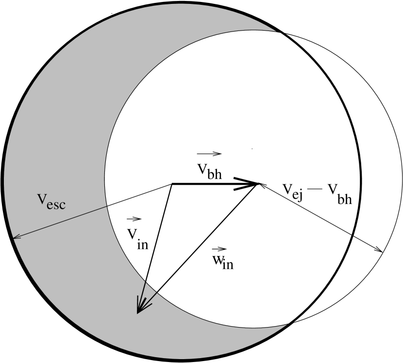
Figure 1.— Velocity-space diagram of gravitational scattering of stars by the IMBH. The initial stellar velocities $\vec{v}_{\rm in}$ lie inside the sphere of radius $v_{\rm esc}$. The stars with velocities in the shadowed region of the figure can be scattered by the IMBH to velocities greater than $v_{\rm ej}$. Other symbols are explained in the text.

Figure 2.— The function $\Lambda(p,q)$ computed for a circular IMBH orbit, $p=1/\sqrt{2}$

Figure 3.— The number of ejected stars as a function of the ejection time. The solid curve represents the region where analytical calculations are appropriate, the dashed curve represents the region where our model is a rough approximation.

Figure 4.— The rate of ejections as a function of the ejection time.

Figure 5.— Scatterplot of velocities and ejection times for the ejected stars

Figure 6.— Dispersion of angles between the ejection velocity vectors and the inspiral plane plotted as a function of ejection time

Figure 7.— Eccentric inspiral: the rate of ejections of stars into GAIA visibility domain as a function of the ejection time. Here the IMBH orbital eccentricity is $e=0.7$.

References

- (1) Artymowicz, P., Lin, D. N. C., & Wampler, E. J. 1993, ApJ, 409, 592
- (2) Brown, W. B., et. al. 2005, ApJ, 622, L33
- (3) Danby, J. M. A. 1988, Fundamentals of Celestial Mechanics, Richmond, Va., USA, Willmann-Bell, 2nd ed.
- (4) Gerhard, O. 2001, ApJ, 546, L39
- (5) Gnedin, O. Y., et. al. 2005, astro-ph/0506739
- (6) Goodman, J., & Tan, J. C. 2004, ApJ, 608, 108
- (7) Gualandris, A., Portegies Zwart, S., & Sipior, M. 2005, accepted to MNRAS, astro-ph/0507365
- (8) Gurkan, M. A., Freitag, M., & Rasio, F. A. 2004, ApJ, 604, 632
- (9) Hansen, B. M. S., & Milosavljevic, M. 2003, ApJ, 593, L77
- (10) Henon, M. 1960a, AnAp, 23, 467
- (11) Henon, M. 1960b, AnAp, 23, 668
- (12) Henon, M. 1969, A&A, 2, 151
- (13) Levin, Y. 2003, astro-ph/0307084
- (14) Levin, Y., & Beloborodov, A. M. 2003, ApJ, 590, L33
- (15) Levin, Y., Wu, A. S. P., Thommes, E. W. 2005, submitted to ApJ, astro-ph/0502143
- (16) Lin, D. N. C., & Tremaine, S. 1980, ApJ, 264, 364
- (17) Morris, M. 1993, ApJ, 408, 496
- (18) Munyaneza, F., Tsiklauri, D., Viollier, R. D. 1999, ApJ, 526, 744
- (19) Phinney, E. S. 1989, in IAU Symp. 136, The Center of the Galaxy, ed. M. Morris (Dordrecht:Kluwer), 543
- (20) Perryman, M. A. C., et. al. 2001, A&A, 369, 339
- (21) Portegies Zwart, S. F., et. al. 2004, Nature, 428, 724
- (22) Sanders, R. H. 1992, Nature, 359, 131
- (23) Shodel, R., et. al. 2005, in preparation
- (24) Young, P. 1980, ApJ, 242, 1232
- (25) Yu, Q., & Tremaine, S. 2003, ApJ, 599, 1129
- (26)