The properties of Ly$\alpha$ emitting galaxies in hierarchical galaxy formation models

Abstract

We present detailed predictions for the properties of Ly$\alpha$-emitting galaxies in the framework of the $\Lambda$CDM cosmology, calculated using the semi-analytical galaxy formation model GALFORM. We explore a model which assumes a top-heavy IMF in starbursts, and which has previously been shown to explain the sub-mm number counts and the luminosity function of Lyman-break galaxies at high redshift. We show that this model, with the simple assumption that a fixed fraction of Ly$\alpha$ photons escape from each galaxy, is remarkably successful at explaining the observed luminosity function of Ly$\alpha$ emitters over the redshift range $3<z<6.6$. We also examine the distribution of Ly$\alpha$ equivalent widths and the broad-band continuum magnitudes of emitters, which are in good agreement with the available observations. We look more deeply into the nature of Ly$\alpha$ emitters, presenting predictions for fundamental properties such as the stellar mass and radius of the emitting galaxy and the mass of the host dark matter halo. The model predicts that the clustering of Ly$\alpha$ emitters at high redshifts should be strongly biased relative to the dark matter, in agreement with observational estimates. We also present predictions for the luminosity function of Ly$\alpha$ emitters at $z>7$, a redshift range which is starting to be be probed by near-IR surveys and using new instruments such as DAzLE.

1 Introduction

After an unpromising start, searches for Ly$\alpha$ emission are now proving to be a powerful means of detecting star-forming galaxies at high redshift (e.g. Hu, Cowie & McMahon, 1998; Pascarelle, Windhorst & Keel, 1998; Kudritzki et al., 2000), competing in observing efficiency with techniques such as broad-band searches for Lyman-break galaxies. The next generation of near-infrared instrumentation (e.g. Horton et al., 2004) will in principle allow Ly$\alpha$ emitting galaxies to be found up to $z\sim 20$, permitting a probe of the star formation history of the Universe before the epoch when reionization is thought to have taken place.

There are in fact a number of different mechanisms which can produce Ly$\alpha$ emission from high redshift objects. (1) Gas in galaxies which is photo-ionized by young stars will emit Ly$\alpha$ as hydrogen atoms recombine; this was originally proposed as a signature of primeval galaxies by Partridge & Peebles (1967). (2) Gas can alternatively be ionized by radiation from an active galactic nucleus (AGN). (3) Intergalactic gas clouds are predicted to emit Ly$\alpha$ recombination radiation due to ionization of the gas by the intergalactic ultraviolet background (e.g. Hogan & Weymann, 1987; Cantalupo et al., 2005). (4) Gas within a dark matter halo which is cooling and collapsing to form a galaxy may radiate much of the gravitational collapse energy by collisionally-excited Ly$\alpha$ emission (e.g. Haiman, Spaans & Quataert, 2000; Fardal et al., 2001). (5) Finally, Ly$\alpha$ can also be emitted from gas which has been shock heated by galactic winds or by jets in radio galaxies (e.g. McCarthy et al., 1987). The majority of high-redshift Ly$\alpha$ emitters (LAEs) detected so far are compact, and appear to be individual galaxies in which the Ly$\alpha$ emission is powered by photoionization of gas by young stars. Ly$\alpha$ surveys have also found another class of emitter, the so-called Ly$\alpha$ blobs, in which the Ly$\alpha$ emission is much more extended than individual galaxies, and may be powered partly by AGNs or gas cooling (Steidel et al., 2000; Bower et al., 2004; Matsuda et al., 2004). We will be focusing in this paper on Ly$\alpha$ emission powered by young stars, and so will not consider the Ly$\alpha$ blobs further.

To date, there has been relatively little theoretical work on trying to predict the properties of star-forming Ly$\alpha$-emitting galaxies within a realistic galaxy formation framework. Haiman & Spaans (1999) made predictions for the number of emitters based on the halo mass function and using ad-hoc assumptions linking Ly$\alpha$ emission to halo mass, while Barton et al. (2004) made predictions for very high redshifts ($z>7$) based on a gas-dynamical simulation. Furlanetto et al. (2005) used gas-dynamical simulations to calculate Ly$\alpha$ emission both from star-forming objects and from the intergalactic medium in the redshift range $0<z<5$. However, the first calculation of the abundance of Ly$\alpha$ emitters based on a detailed hierarchical galaxy formation model was that of Le Delliou et al. (2005, hereafter Paper I). In Paper I, we used the GALFORM semi-analytical galaxy formation model to predict the abundance of star-forming Ly$\alpha$ emitters as a function of redshift in the cold dark matter (CDM) model. The GALFORM model computes the assembly of dark matter halos by mergers, and the growth of galaxies both by cooling of gas in halos and by galaxy mergers. It calculates the star formation history of each galaxy, including both quiescent star formation in galaxy disks and also bursts triggered by galaxy mergers, as well as the feedback effects of galactic winds driven by supernova explosions. In Paper I, we found that a very simple model, in which a fixed fraction of Ly$\alpha$ photons escape from each galaxy, regardless of its other properties, gave a surprisingly good match to the total numbers of Ly$\alpha$ emitters detected in different surveys over a range of redshifts. We also explored the impact of varying certain parameters in the model, such as the redshift of reionization of the intergalactic medium, on the abundance of emitters.

In this paper, we explore in more detail the fiducial model of Paper I (based on an $\Omega_{m}=0.3$, spatially flat, $\Lambda$CDM model with a reionization redshift of $10$). We use the full capability of the GALFORM model to predict a wide range of galaxy properties, connecting various observables to Ly$\alpha$ emission. The galaxy formation model we use is the same as that proposed by Baugh et al. (2005). A critical assumption of this model is that stars formed in starbursts have a top-heavy initial mass function (IMF), while stars formed quiescently in galactic disks have a solar neighbourhood IMF. We showed in Baugh et al. that, within the framework of $\Lambda$CDM, the top-heavy IMF is essential for matching the counts and redshifts of sub-millimetre galaxies and the luminosity function of Lyman break galaxies at $z=3$ (once dust extinction is included), while remaining consistent with galaxy properties in the local universe such as the optical and far-IR luminosity functions and galaxy gas fractions and metallicities. More detailed comparisons of this model with observations of Lyman-break galaxies and of galaxy evolution in the IR will be presented in Lacey et al. (2005a, 2005b, in preparation). The assumption of a top-heavy IMF is controversial, but underpins the success of the model in explaining the high-redshift sub-mm and Lyman-break galaxies. It is therefore important to test this model against as many observables as possible. Nagashima et al. (2005a) showed that a top-heavy IMF seems to be required to explain the metal content of the hot intracluster gas in galaxy clusters, and Nagashima et al. (2005b) showed that a similar top-heavy IMF also seems to be necessary to explain the observed abundances of $\alpha$-elements (such as Mg) in the stellar populations of elliptical galaxies. In the present paper, we explore the predictions of the Baugh et al. (2005) model for the properties of Ly$\alpha$-emitting galaxies and compare them with observational data. We emphasize that our aim here is to explore in detail a particular galaxy formation model which has been shown to satisfy a wide range of other observational constraints, rather than to conduct a survey of Ly$\alpha$ predictions for different model parameters.

In Section 2, we give an outline of the GALFORM model, focusing on how the predictions we present later on are calculated. Section 3 examines the evolution of the Ly$\alpha$ luminosity function, and compares the model predictions with observational data over the redshift range $3\la z\la 7$. In Section 4, we compare a selection of observed properties of Ly$\alpha$ emitters with the model predictions. In Section 5, we look at some other predictions of the model, most of which cannot currently be compared directly with observations. Section 6 extends the predictions for the Ly$\alpha$ luminosity function to $z>7$. We present our conclusions in Section 7 .

2 Galaxy formation model

We use the semi-analytical model of galaxy formation, GALFORM, to predict the Ly$\alpha$ emission and many other properties of galaxies as a function of redshift. The general methodology and approximations behind the GALFORM model are set out in detail in Cole et al. (2000). The particular model that we use in this paper is the same as that described by Baugh et al. (2005). The background cosmology is a cold dark matter universe with a cosmological constant ($\Omega_{m}=0.3$, $\Omega_{\Lambda}=0.7$, $\Omega_{b}=0.04$, $h\equiv H_{0}/100{\rm km\,s^{-1}}{\rm Mpc}^{-1}=0.7$, $\sigma_{8}=0.93$). Below we review the physics behind the particular model predictions that we highlight in this paper.

The GALFORM model follows the main processes which shape the formation and evolution of galaxies. These include: (i) the collapse and merging of dark matter halos; (ii) the shock-heating and radiative cooling of gas inside dark halos, leading to formation of galaxy disks; (iii) quiescent star formation in galaxy disks; (iv) feedback both from supernova explosions and from photo-ionization of the IGM; (v) chemical enrichment of the stars and gas; (vi) galaxy mergers driven by dynamical friction within common dark matter halos, leading to formation of stellar spheroids, and also triggering bursts of star formation. The end product of the calculations is a prediction of the number of galaxies that reside within dark matter haloes of different masses. The model predicts the stellar and cold gas masses of the galaxies, along with their star formation and merger histories, and their sizes and metallicities.

The prescriptions and parameters for the different processes which we use in this paper are identical to Baugh et al. (2005). Feedback is treated in a similar way to Benson et al. (2003): energy injection by supernovae reheats some of the gas in galaxies and returns it to the halo, but also ejects some gas from halos as a “superwind” - the latter is essential for reproducing the observed cutoff at the bright end of the present-day galaxy luminosity function. We also include feedback from photo-ionization of the IGM: following reionization (i.e. for $z<z_{\rm reion}$), we assume that gas cooling in halos with circular velocities $V_{c}<60\,{\rm km\,s^{-1}}$ is completely suppressed. We assume in this paper that reionization occurs at $z_{\rm reion}=10$, chosen to be intermediate between the low value $z\sim 6$ suggested by measurements of the Gunn-Peterson trough in quasars (Becker et al. , 2001) and the high value $z\sim 20$ suggested by the WMAP measurement of polarization of the microwave background (Kogut et al. , 2003). Our model has two different IMFs: quiescent star formation in galactic disks is assumed to produce stars with a solar neighbourhood IMF (we use the Kennicutt (1983) paramerization, with slope $x=0.4$ below $1M_{\odot}$ and $x=1.5$ above), whereas bursts of star formation triggered by galaxy mergers are assumed to form stars with a top-heavy, flat IMF with slope $x=0$ (where the Salpeter slope is $x=1.35$). In either case, the IMF covers the mass range $0.15<m<120M_{\odot}$. As mentioned in the Introduction, the choice of a flat IMF in bursts is essential for the model to reproduce the observed counts of galaxies at sub-mm wavelengths. The parameters for star formation in disks and for triggering bursts and morphological transformations in galaxy mergers are given in Baugh et al. (2005).

The sizes of galaxies are computed as in Cole et al. (2000): gas which cools in a halo is assumed to conserve its angular momentum as it collapses, forming a rotationally-supported galaxy disk; the radius of this disk is then calculated from its angular momentum, including the gravity of the disk, spheroid (if any) and dark halo. Galaxy spheroids are built up both from pre-existing stars in galaxy mergers, and from the stars formed in bursts triggered by these mergers; the radii of spheroids formed in mergers are computed using an energy conservation argument. In calculating the sizes of disks and spheroids, we include the adiabatic contraction of the dark halo due to the gravity of the baryonic components.

Given the star formation and metal enrichment history of a galaxy, GALFORM computes the spectrum of the integrated stellar population using a population synthesis model based on the Padova stellar evolution tracks (see Granato et al., 2000, for details). Broad-band magnitudes are then computed by redshifting the galaxy spectrum and convolving it with the filter response functions. We include extinction of the stellar continuum by dust in the galaxy; this is computed based on a two-phase model of the dust distribution, in which stars are born inside giant molecular clouds and then leak out into a diffuse dust medium (see Granato et al., 2000, for more details). The optical depth for dust extinction of the diffuse component is calculated from the mass and metallicity of the cold gas and the sizes of the disk and bulge. We note that the extinction predicted by our model in which the stars and dust are mixed together is very different from what one obtains if all of the dust is in a foreground screen (as is commonly assumed in other theoretical models). Finally, we also include the effects on the observed stellar continuum of absorption and scattering of radiation by intervening neutral hydrogen along the line of sight to the galaxy; we calculate this IGM attenuation using the formula of Madau (1995), which is based on the observed statistics of neutral hydrogen absorbers seen in quasar spectra.

We compute the Ly$\alpha$ luminosities of galaxies by the following procedure: (i) The model calculates the integrated stellar spectrum of the galaxy as described above, based on its star formation history, and including the effects of the distribution of stellar metallicities and of variations in the IMF. (ii) We compute the rate of production of Lyman continuum (Lyc) photons by integrating over the stellar spectrum, and assume that all of these ionizing photons are absorbed by neutral hydrogen within the galaxy. We assume photoionization equilibrium applies within each galaxy, producing Ly$\alpha$ photons according to case B recombination (e.g. Osterbrock, 1989). We note that for solar metallicity, 11 times as many Lyc and Ly$\alpha$ photons are produced per unit mass of stars formed for our top-heavy (burst) IMF as compared to our solar neighbourhood (disk) IMF. (iii) The observed Ly$\alpha$ flux or luminosity of a galaxy depends on the fraction $f_{\rm esc}$ of Ly$\alpha$ photons which escape from the galaxy. Ly$\alpha$ photons are resonantly scattered by neutral hydrogen, and absorbed by dust. Early estimates of this process (e.g. Charlot & Fall, 1991) showed that only a tiny fraction of Ly$\alpha$ photons should escape from a static neutral galaxy ISM if even a tiny amount of dust is present. Many star-forming galaxies are nonetheless observed to have significant Ly$\alpha$ luminosities (e.g. Kunth et al. , 1998; Pettini et al. , 2001), and this is generally ascribed to the presence of galactic winds in these systems, which allow Ly$\alpha$ photons to escape after many fewer resonant scatterings. Radiative transfer calculations of Ly$\alpha$ through winds have shown that this process can explain the asymmetric Ly$\alpha$ line profiles which are typically observed (e.g. Ahn, 2004). The effects of radiative transfer of Ly$\alpha$ through clumpy dust and gas have been considered by Neufeld (1991) and Hansen & Oh (2005).

Calculating Ly$\alpha$ escape fractions from first principles is clearly very complicated, and so we instead adopt a simpler approach. In Paper I, we found that assuming a fixed escape fraction $f_{\rm esc}$ for each galaxy, regardless of its dust properties, resulted in a surprisingly good agreement between the predicted number counts of emitters and the available observations. In that paper, we chose $f_{\rm esc}=0.02$ to match the number counts at $z\approx 3$ at a flux $f\approx 2\times 10^{-17}{\rm erg\,s^{-1}}$, and we use the same value of $f_{\rm esc}$ in this paper. Although this extreme simplification of a constant escape fraction may seem implausible, it does give a reasonably good match to the observed Ly$\alpha$ luminosity functions and equivalent widths at different redshifts, as we show in the next sections.

Our calculations do not include any attenuation of the Ly$\alpha$ flux from a galaxy by propagation through the IGM. Ly$\alpha$ photons can be scattered out of the line-of-sight by any neutral hydrogen in the IGM close to the galaxy. If the emitting galaxy is at a redshift before reionization, when the IGM was still mostly neutral, this could in principle strongly suppress the observed Ly$\alpha$ flux (Miralda-Escude, 1998). However, various effects can greatly reduce the amount of attenuation: ionization of the IGM around the galaxy (Madau & Rees, 2000; Haiman, 2002), clearing of the IGM by galactic winds, gravitational infall of the IGM towards the galaxy, and redshifting of the Ly$\alpha$ emission by scattering in a wind (Santos, 2004). In any case, since measurements of Gunn-Peterson absorption in quasars show that reionization must have occured at $z\ga 6.5$, attenuation of Ly$\alpha$ fluxes by the IGM should not affect our predictions for $z\la 6.5$, but only our predictions for very high redshifts given in Section 6.

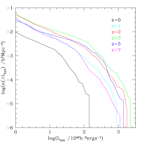
Figure 1: The predicted evolution with redshift of the cumulative Ly$\alpha$ luminosity function, defined as the comoving number density of galaxies with Ly$\alpha$ luminosities brighter than $L_{Ly\alpha}$. The model predictions are shown for selected redshifts in the interval $z=0$ to $z=7$.

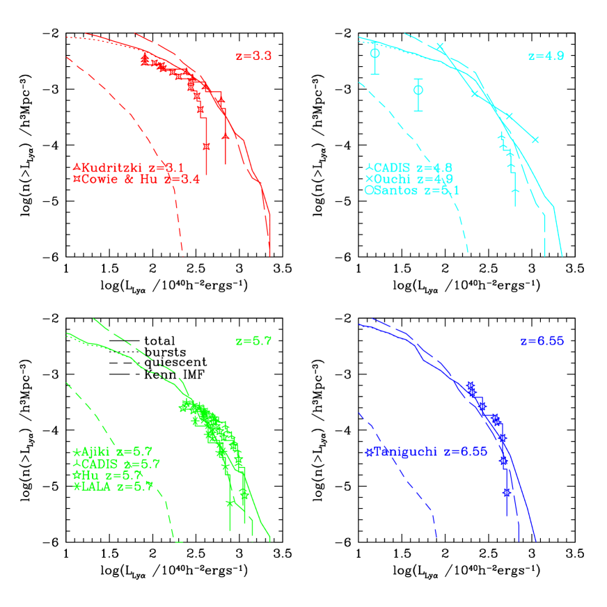
Figure 2: The evolution of the cumulative Ly$\alpha$ luminosity function with redshift, comparing models with observational data. Each panel corresponds to a different redshift, as indicated by the legend. The curves show model predictions, while the lines with symbols and symbols with error bars show observational data. The solid curves show the predictions for the total luminosity function for our standard model, with a top-heavy IMF in bursts and $f_{\rm esc}=0.02$, while the dotted and short-dashed lines show the separate contributions of starbursts and quiescently star-forming galaxies respectively (in most cases the solid and dotted lines overlap). The long-dashed curves show the predicted total luminosity function for a variant model with a universal Kennicutt IMF and $f_{\rm esc}=0.2$. The references for the observational data (as shown in the symbol key) are as follows: Kudritzki - Kudritzki et al. (2000); Cowie & Hu - Cowie & Hu (1998); CADIS - Maier et al. (2003); Ouchi - Ouchi et al (2003); Santos - Santos et al.  (2004); Ajiki - Ajiki et al. (2003); Hu - Hu et al. (2004); LALA - Rhoads et al. (2003); Taniguchi - Taniguchi et al. (2005). The redshifts for the observational data are close to that of the model plotted in each panel, but do not exactly coincide in all cases. In most cases, the data are plotted as stepped histograms, with each step corresponding to a single galaxy.

3 Evolution of the Ly$\alpha$ luminosity function

A basic prediction of our model is the evolution of the luminosity function of Ly$\alpha$ emitters with redshift. This depends on the distribution of star formation rates in quiescent and starburst galaxies (with solar neighbourhood and top-heavy IMFs respectively), and on the metallicity with which the stars are formed. Paper I showed predictions for the cumulative number counts of emitters per unit redshift as a function of observed Ly$\alpha$ flux. Here we focus on a closely related quantity, the cumulative space density of emitters as a function of Ly$\alpha$ luminosity at different redshifts. Fig.1 shows the cumulative luminosity function of Ly$\alpha$ emitters predicted by our standard model for a set of redshifts over the interval $z=0-7$. The model luminosity function initially gets brighter with increasing redshift, peaking at $z=3$, before declining again in number density at even higher redshifts. The increase in the luminosity function from $z=0$ to $z\sim 3$ is driven both by the increase in galaxy star formation rates, and by the increasing fraction of star formation occuring in bursts (which have a top-heavy IMF). As shown in Fig.1 in Baugh et al. (2005), the model predicts that the fraction of all star formation occuring in bursts increases from $\sim 5\%$ at $z=0$ to $50\%$ at $z\sim 3.5$ and then to $\sim 80\%$ at $z\ga 6$.

We compare the model predictions with observational estimates of the cumulative Ly$\alpha$ luminosity function in Fig.2, where we show different redshifts in different panels. The observational estimates of the luminosity functions which we plot have been calculated by Tran et al. (2004) (and also S. Lilly, private communication, for $z=6.55$) from published data on surveys for LAEs, assuming the same cosmology as we assume in our models. The observed luminosity functions in the figures are labelled according to the survey from which they were obtained. In each case, surveys using narrow-band filters were used to find candidates for LAEs at particular redshifts, and then either broad-band colours or follow-up spectroscopy were used to determine which of the candidates were likely to be real Ly$\alpha$ emitters, and which were likely to be lower-redshift interlopers resulting from other emission lines falling within the narrow-band filter response. The surveys with spectroscopic follow-up which we plot are Kudritzki et al. (2000), Cowie & Hu (1998), Hu et al. (2004), Rhoads et al. (2003, LALA) and Taniguchi et al. (2005), while the surveys using only colour selection are Maier et al. (2003, CADIS), Ouchi et al (2003) and Ajiki et al. (2003). We also show the data of Santos et al.  (2004) at $z\approx 5$ from a spectroscopic survey of gravitationally-lensed fields. The stepped appearance of most of the observed luminosity functions results from the small number of objects in most of the samples; each step corresponds to the inclusion of an additional object as the luminosity is reduced. The cumulative luminosity functions cut off at the bright end where the observational samples contain only one object of that luminosity; the statistical uncertainties are correspondingly largest at the highest luminosities. For reference, we note that the luminosity distance for our assumed cosmology is $d_{L}=(2.0,3.2,3.8,4.5)\times 10^{4}h^{-1}{\rm Mpc}$ for $z=3.3,4.9,5.7,6.55$ respectively, so that a Ly$\alpha$ flux of $10^{-17}{\rm erg\,cm^{-2}s^{-1}}$ at each of these redshifts corresponds to a luminosity $(0.5,1.2,1.7,2.4)\times 10^{42}h^{-2}{\rm erg\,s^{-1}}$ respectively. The lower luminosity limits on the observed luminosity functions correspond to roughly the same Ly$\alpha$ flux limit $\sim 10^{-17}{\rm erg\,cm^{-2}s^{-1}}$ at each redshift.

In Fig.2, the predictions for our standard model (with a top-heavy IMF in bursts and $f_{\rm esc}=0.02$) are shown by solid lines. We also show the separate contributions of bursting and quiescently star-forming galaxies respectively as dotted and short-dashed lines. In most cases, the dotted line is barely distinguishable from the solid line, showing that the model Ly$\alpha$ luminosity function is completely dominated by bursts over the range of redshift and luminosity plotted in Fig.2. Overall, there is broad agreement between the predicted and observed luminosity functions over the redshift range $z=3-6.6$. This is remarkable, since we allowed ourselves to adjust only one model parameter to fit the observational data, namely the Ly$\alpha$ escape fraction $f_{\rm esc}$. The model luminosity functions do not perfectly match all of the observational data, but where there are differences between the model and observational data, there are also equally large differences between different observational datasets. The differences between different observational datasets could be due to a combination of (a) statistical fluctuations (most of the samples are small), (b) field-to-field variance due to galaxy clustering (e.g. Ouchi et al, 2003; Shimasaku et al., 2003), (c) differences in the details of how the samples are selected (e.g. differences in the equivalent width limit or photometric criteria applied), and (d) differing levels of contamination by objects which are not Ly$\alpha$ emitters. We note that the model predictions shown in Fig.2 do not include any limit on the equivalent width (EW) of the Ly$\alpha$ emission line, while the observational data shown all incorporate different lower limits on the EW of line emission as well as on the line flux. However, as we show in §4.1, these EW thresholds are predicted not to significantly affect the comparison of model and observed luminosity functions in Fig.2.

The value of the Ly$\alpha$ escape fraction which we find fits the data, $f_{\rm esc}=0.02$, is quite small. This is mainly because, over the range of redshift and luminosity probed by the observations, the counts of objects in our standard model are dominated by bursts, and we have assumed a top-heavy IMF in bursts. As noted above, the Ly$\alpha$ luminosity for a given star formation rate is about 10 times larger with the top-heavy IMF than with a solar neighbourhood IMF. We also show in Fig.2 by long-dashed lines the predictions of a variant model, in which we assume the same Kennicutt IMF for bursts and quiescent star formation, and with $f_{\rm esc}=0.2$. Even though we have chosen $f_{\rm esc}$ for this variant model to provide the best overall match to the observational data in Fig.2, we see that it agrees somewhat less well with the data than does our standard model, especially at $z=3.3$, where it predicts more low-luminosity galaxies. Moreover, this variant model dramatically under-predicts both the counts of sub-mm galaxies and the number of Lyman-break galaxies (see Fig.5(a) in Baugh et al. (2005)).

We have also investigated the effect on the predicted luminosity functions of changing the IGM reionization redshift from our standard value $z_{\rm reion}=10$. As described in §2, this affects galaxies in our model through photo-ionization feedback. For our standard model, we find that varying $z_{\rm reion}$ over the range 6.5 to 20 changes the luminosity function by less than the scatter between different observational datasets in Fig.2, over the range of luminosity and redshift probed by those data. Choosing a different value of $z_{\rm reion}$ in this range would therefore not significantly affect any of the conclusions we draw here.

Furlanetto et al. (2005) have computed luminosity functions of Ly$\alpha$ emitters from a numerical simulation, including emission from gas heated by shocks and by the intergalactic ionizing background as well as emission from star-forming regions in galaxies. They assume that stars all form with a Salpeter IMF. However, the luminosity functions which they compute combine all of the emission from each dark matter halo, and so are different from the luminosity functions of individual galaxies which our model predicts. Furthermore, they effectively assume an escape fraction $f_{\rm esc}=1$ for Ly$\alpha$ emission from star formation. They do not make any detailed comparison with observational data on Ly$\alpha$-emitting galaxies, but note that their luminosity functions predict roughly an order-of-magnitude more objects than are observed over the range $L_{Ly\alpha}\sim 10^{42}-10^{43}{\rm erg\,s^{-1}}$. This is roughly consistent with what we would find if we assumed a Kennicutt IMF for all star formation and $f_{\rm esc}=1$.

4 Observable properties of Ly$\alpha$ emitters

Now that we have established that our model gives a very good match to the luminosity function of Ly$\alpha$ emitters at different redshifts, we turn our attention to other observable properties of these objects. We first present predictions for the distribution of Ly$\alpha$ equivalent widths (§4.1), before examining the broad-band continuum magnitudes of Ly$\alpha$ emitters (§4.2) and, finally, the size distribution of emitters (§4.3).

4.1 Ly$\alpha$ equivalent widths

Our model allows a simple prediction for the equivalent width (EW) of the Ly$\alpha$ emission line in each galaxy: we divide the luminosity in the emission line by the mean luminosity per unit wavelength of the stellar continuum on either side of the line. We distinguish between the net and intrinsic line and stellar luminosities and equivalent widths. The net values are obtained after we multiply the Ly$\alpha$ luminosity by the escape fraction $f_{\rm esc}$ and after we attenuate the stellar luminosity by dust extinction, while the intrinsic values are those before we include either the Ly$\alpha$ escape fraction or dust attenuation. A limitation of our current model is that it does not include the effects of absorption of Ly$\alpha$, so the equivalent widths we calculate are always positive (or zero). Ly$\alpha$ absorption features (corresponding to negative equivalent widths) could be produced either by absorption in stellar atmospheres (Charlot & Fall, 1993), or by neutral gas within the galaxy or in an expanding shell or wind around it (Tenorio-Tagle et al., 1999). Our calculations are therefore incomplete, but nevertheless represent an important first step.

Fig.3 shows the model predictions for rest-frame equivalent widths of Ly$\alpha$-emitting galaxies at z=3. The most remarkable feature of these plots is the wide spread of EWs predicted by the model. This is seen most clearly in the middle panel, which shows the distribution of equivalent widths for galaxies selected to have Ly$\alpha$ fluxes in the range $10^{-17}<f<10^{-16}{\rm erg\,cm^{-2}s^{-1}}$. We see that there is a big difference between the distributions of intrinsic and net EWs (shown by dashed and solid lines respectively). For this flux range, the intrinsic rest-frame EW has a median value of 130Å, and most galaxies have EWs in the range 100–200Å. These values are similar to the predictions of Charlot & Fall (1993). The spread in intrinsic EWs results mostly from the spread in burst ages and timescales. For the same galaxies, the net EWs have a much lower median value, 33Å, but with a much broader distribution, with a peak close to 0 and a tail extending up to $\sim 400$Å. Since our model assumes that all galaxies have the same escape fraction for Ly$\alpha$, this broad distribution of net EWs results from the wide spread in values of dust extinction for the stellar continuum. The Ly$\alpha$ escape fraction reduces the net EW relative to the intrinsic value, but dust extinction of the stellar continuum increases it.

The upper panel of Fig.3 shows the median and 10-90 percentile range for the EW of Ly$\alpha$ as a function of the net Ly$\alpha$ flux. There is a weak trend of EW increasing with Ly$\alpha$ flux (or luminosity). In the case of the intrinsic EW, this increase is driven mostly by the shift from being dominated by quiescently star-forming galaxies (with a normal IMF) at low luminosities to being dominated by bursts (with a top-heavy IMF) at high luminosities, and by the change in the typical star formation history. For the net EW, the increase in the median is driven also by the increase in the typical dust extinction of the stellar continuum with increasing luminosity.

The Ly$\alpha$ equivalent widths predicted by our model are similar to those found in observed galaxy samples selected by their Ly$\alpha$ emission. Cowie & Hu (1998) and Kudritzki et al. (2000) selected LAEs having Ly$\alpha$ fluxes $\sim 10^{-17}-10^{-16}{\rm erg\,cm^{-2}s^{-1}}$ at $z=3.4$ and $z=3.1$ respectively. In both cases, their narrow-band selection imposed a lower limit on the rest-frame EW $\approx 20$Å for the detected objects, and the median rest-frame EW of the objects above this threshold was found to be $\approx 40$Å. This appears broadly compatable with the predictions shown in Fig.3, once one allows for the fact that the EW threshold in the observed samples will raise the median EW above the value expected in the absence of any EW threshold. At a higher redshift, $z\approx 4.5$, Dawson et al.  (2004) selected LAEs with $f\sim 10^{-17}-10^{-16}{\rm erg\,cm^{-2}s^{-1}}$ and $EW({\rm rest})>15$Å, and measured a median $EW({\rm rest})\approx 80$Å for their sample. This is also in good agreement with our model, which predicts a median $EW({\rm rest})\approx 80$Å for LAEs with $10^{-17}<f<10^{-16}{\rm erg\,cm^{-2}s^{-1}}$ at this redshift.

Figure 3: The predicted rest-frame equivalent width (EW) of the Ly$\alpha$ emission line for galaxies at $z=3$. We show results both for the intrinsic EW, i.e. before including attenuation by neutral gas and dust in the galaxy, and for the net EW, i.e. after including the escape fraction for Ly$\alpha$ photons and dust extinction of the stellar continuum - these are shown by dashed and solid lines respectively. In either case, the EW is considered as a function of the net Ly$\alpha$ flux. (a) The upper panel shows the predicted median EW as a function of the net Ly$\alpha$ flux. The error bars show the 10-90 percentile range at a given flux. (b) The middle panel shows the predicted distribution of EWs for galaxies with net Ly$\alpha$ fluxes in the range $10^{-17}-10^{-16}{\rm erg\,cm^{-2}s^{-1}}$. (c) The lower panel shows the predicted EW distribution for galaxies selected to have continuum magnitudes in the range $23<R_{AB}<25.5$.

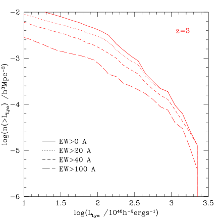
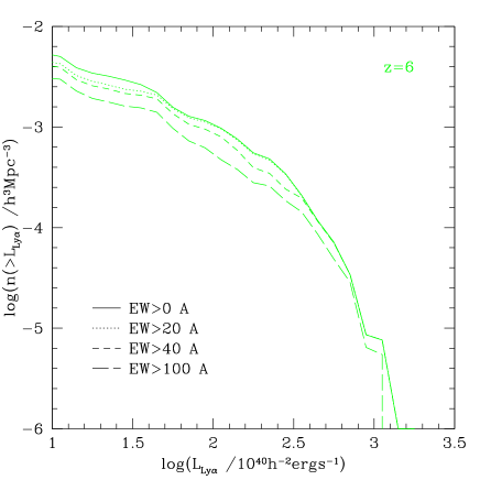
Figure 4: The effect of different equivalent width thresholds on the predicted luminosity function of Ly$\alpha$ emitters. In each panel, the lines show the predicted cumulative luminosity function for different lower limits on the rest-frame EW of Ly$\alpha$ emission: EW$>0$Å (solid curves), EW$>20$Å (dotted), EW$>40$Å (short-dashed), and EW$>100$Å (long-dashed). (a) $z=3$. (b) $z=6$.

Shapley et al.  (2003) have measured Ly$\alpha$ emission and absorption profiles and EWs in a sample of galaxies at $z\sim 3$ selected using the Lyman-break technique. Their sample is thus selected on rest-frame far-UV stellar continuum luminosity, rather than on the presence of a strong Ly$\alpha$ emission line. They find that $\sim 30\%$ of their galaxies show Ly$\alpha$ only in emission, $\sim 30\%$ of galaxies show Ly$\alpha$ only in absorption, and $\sim 40\%$ show a combination of Ly$\alpha$ absorption and emission. They find a very asymmetric and skewed distribution of Ly$\alpha$ rest-frame EW’s, with a median close to 0Å, extending down to $\sim-50$Å for net absorption and to $\ga 100$Å for net emission. For the galaxies with net Ly$\alpha$ emission, the median EW is $\sim 20$Å. (For galaxies with net absorption, the median EW is $\sim-20$Å.) The lower panel of Fig.3 shows the EW distribution predicted by the model if we select galaxies in a similar way to Shapley et al. , with a continuum magnitude range $23<R_{AB}<25.5$ (including dust extinction) and no condition on the Ly$\alpha$ flux or EW. The model predicts a median EW $\approx 20$Å for this case, very similar to the typical EW of the emission component of Ly$\alpha$ in the Shapley et al.  sample. The shape of the model EW distribution (which is restricted to EW $\geq 0$) is also very similar to that found by Shapley et al.  for $EW>0$ (see their Fig.8). However, without including a calculation of Ly$\alpha$ absorption in our model, we cannot make a more detailed comparison with Shapley et al. . Since a calculation of Ly$\alpha$ absorption requires a treatment of radiative transfer through the galaxy ISM, we defer this to a future paper.

Since our model allows us to estimate Ly$\alpha$ EWs, we can also estimate the effect on the Ly$\alpha$ luminosity function of imposing different lower limits on the EWs of Ly$\alpha$ emission from galaxies. This is shown in Fig.4, for rest-frame EW thresholds $EW_{\rm min}({\rm rest})=0,20,40$ and $100$Å, for redshifts $z=3$ and $z=6$. Different observational surveys for LAEs impose different lower limits on the EWs of the objects they include. However, for most of the observational data plotted in Fig.2, the lower limit is around $EW_{\rm min}({\rm rest})=20$Å. We see from Fig.4 that an EW threshold around this value is predicted to have only a small effect on the Ly$\alpha$ luminosity function, so the conclusions we drew from the comparison with observational data in Fig.2 would not be significantly affected.

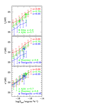
Figure 5: Broad-band magnitudes as a function of Ly$\alpha$ flux. The lines show the model predictions for three different redshifts, $z=3$, 5.7 and 6.55, in different colours. The dashed lines show the median magnitude due to the stellar continuum only, while the solid lines include also the contribution of the Ly$\alpha$ line to the broad-band magnitude. Where the dashed line is not visible, it coincides with the solid line. The error bars on the lines show the 10-90 percentile range. For clarity, small offsets in the $x$-direction have been applied to the model relations for different redshifts. The top, middle and lower panels show results for the $I_{c}$, $i^{\prime}$ and $z^{\prime}$ filters respectively. The symbols show observational data, plotted in the same colours as the model curve closest in redshift. The observational data are as follows: Ellis - Ellis et al. (2001) (1 galaxy); Ajiki - Ajiki et al. (2003) (20 galaxies); Stanway - Stanway et al. (2004) (3 galaxies); Taniguchi - Taniguchi et al. (2005) (9 galaxies). For samples with $>1$ galaxy, we plot an estimate of the median Ly$\alpha$ flux and broad-band magnitude, and of the 10-90 percentile ranges in both (shown by error bars).

4.2 Broad-band magnitudes

Another important test for our model of the Ly$\alpha$ emitters is that it should predict the correct stellar continuum as measured in broad-band filters. Fig.5 shows the model predictions for the median broad-band magnitudes as a function of Ly$\alpha$ flux at three different redshifts, $z=3$, 5.7 and 6.55, and for three different broad-band filters, the $I_{c}$, $i^{\prime}$ and $z^{\prime}$ filters on the Suprime Cam on the Subaru Telescope. (We chose these particular filters because most of the observational data we will compare with were taken with them.) The predicted broad-band magnitudes include the effects of dust extinction and of attenuation by the intervening IGM (based on Madau 1995). The evolution with redshift of the predicted $I_{c}$ and $i^{\prime}$ magnitudes at a given Ly$\alpha$ flux which is seen in Fig.5 results mostly from the IGM opacity. In some cases, the Ly$\alpha$ emission line falls within the bandpass of the filter. We have therefore computed broad-band magnitudes due to either the stellar continuum only (shown by dashed lines), or to the stellar continuum and Ly$\alpha$ emission line together (shown by solid lines). In most of the cases plotted in Fig.5, the solid and dashed lines are indistinguishable, but in a few cases there is a small offset, showing that the Ly$\alpha$ line makes a modest contribution to the broad-band magnitude in these cases.

For comparison, we also plot in Fig.5 a selection of observational data for galaxies at $z\sim 5-7$ from the following papers: Ellis et al. (2001), Ajiki et al. (2003), Stanway et al. (2004) and Taniguchi et al. (2005). The data we plot constrain the stellar continuum at wavelengths $\sim 900-1400$Å in the galaxy rest-frame. The Ellis et al. and Stanway et al. data were actually taken on HST using the WFPC2 ($I_{814}$ filter) and ACS ($i^{\prime}$ and $z^{\prime}$ filters) cameras respectively, but we have verified that the difference of these filters from the Subaru filters (in particular, the difference of $I_{814}$ from $I_{c}$) does not significantly affect the comparison of models with data which we make here. In cases where the observational papers have tried to correct the broad-band magnitudes for the contribution from the Ly$\alpha$ line, we have plotted the total magnitude before this correction was made. We plot the observational data in Fig.5 as symbols of the same colour as the model curve closest in redshift. Apart from Ellis et al., all of the samples contain more than one galaxy, and in these cases we estimate the median and 10-90% percentile range for both the Ly$\alpha$ flux and the broad-band magnitude (allowing for upper limits on the broad-band fluxes). We plot the symbol at the median value and show the 10-90% range by error bars. If the 10% value is an upper limit, we indicate this by a very long downwards error bar.

We see from Fig.5 that there is mostly good agreement between the predicted broad-band magnitudes and the observational data. The one exception is that the median $i^{\prime}$ magnitude measured from Taniguchi et al. (2005) for galaxies at $z=6.55$ is nearly 3 magnitudes brighter than what our model predicts, even though the $z^{\prime}$ magnitudes for the same observational sample agree very well with the model predictions. However, 7 out of 9 objects in the Taniguchi et al. sample are detected in the $i^{\prime}$ band at less than $2\sigma$ significance, so it is possible that the symbol marking our estimate of their median magnitude is biased high by statistical errors. We note that at redshift $z=6.55$, the $i^{\prime}$-band flux is sensitive to emission at wavelengths $\sim 900-1100$Å in the galaxy rest-frame, so it is expected to be greatly attenuated by Ly$\alpha$ absorption by neutral hydrogen in the intervening IGM. In contrast, the flux in the $z^{\prime}$ band at this redshift is expected to be much less affected by IGM attenuation. Thus, an alternative possible explanation for the disagreement between the model and the Taniguchi et al. $i^{\prime}$ data is that we over-estimate the degree of IGM attenuation at this redshift when we calculate it using the Madau (1995) formula.

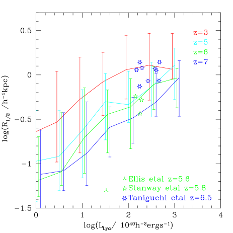
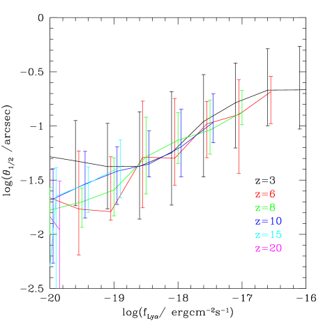
Figure 6: The sizes of Ly$\alpha$ emitters. (a) The top panel shows the physical sizes of Ly$\alpha$ emitters as a function of their Ly$\alpha$ luminosities. The lines show model predictions for the median stellar half-mass radius for four different redshifts, $z=3$, 5, 6 and 7. The error bars show the 10-90 percentile range at a given luminosity. The symbols show observational estimates of galaxy radii, from Ellis et al. (2001), Stanway et al. (2004) and Taniguchi et al. (2005), plotted for individual galaxies in the same colours as the model curve closest in redshift (see text for more details). (b) The lower panel shows predicted angular sizes as a function of Ly$\alpha$ flux, for the redshifts $z=3,6,8,10,15$ and $20$. The sizes plotted are again stellar half-mass radii.

4.3 Sizes of Ly$\alpha$ emitters

Our semi-analytical model predicts the half-mass radii for the disk and bulge components of each galaxy. From these we can compute the half-mass radius of the stars, and also half-light radii in different bands, allowing for different colours of the disk and bulge, but assuming that both components have internally uniform colours. Coenda et al. (2005, in preparation) will present predictions from our model for the sizes of galaxies selected by their stellar continuum emission, and compare with observational data over the redshift range $0<z<6$. Cole et al. (2000) have discussed predictions for galaxy sizes at $z=0$ based on an earlier version of our semi-analytical model. In the present paper, we will only consider the sizes of galaxies selected to be Ly$\alpha$ emitters. We emphasize that we are not considering in this paper the properties of Ly$\alpha$ blobs (e.g. Matsuda et al., 2004), which are much more spatially extended than typical Ly$\alpha$ emitters, and appear to be a distinct class of object.

In Fig.6(a), we show model predictions for the median stellar half-mass radius (together with its 10-90 percentile range) as a function of Ly$\alpha$ luminosity for several different redshifts, $z=3$, 5, 6 and 7. We have also calculated model half-light radii in the rest-frame UV, and the results are almost identical to those for the half-mass radius for these redshifts and luminosities. The stellar sizes are predicted to be quite compact at these redshifts, $\la 1h^{-1}{\rm kpc}$. We see that, as well as a correlation of size with luminosity (roughly as $R_{1/2}\propto L^{1/3}$), the models also predict that the median radius at a given luminosity should decrease with increasing redshift (roughly as $(1+z)^{-1}$ or $(1+z)^{-1.5}$). At a fixed Ly$\alpha$ luminosity of $10^{42.5}h^{-2}{\rm erg\,s^{-1}}$ (the typical value in the higher-redshift surveys shown in Fig.2), the median half mass radius shrinks from $\sim 1h^{-1}{\rm kpc}$ at $z=3$ to $\sim 0.5h^{-1}{\rm kpc}$ at $z=7$.

We have also plotted in Fig.6(a) some observational estimates of sizes for individual Ly$\alpha$-emitting galaxies at $z\sim 5-7$, plotted in the same colour as the model curve closest in redshift, for three different samples: Stanway et al. (2004) used HST to measure half-light radii in the rest-frame UV of 3 LAEs; Ellis et al. (2001) used HST to measure the rest-frame UV size of a single strongly gravitationally lensed LAE; and Taniguchi et al. (2005) used ground-based narrow-band imaging to estimate the sizes of the Ly$\alpha$-emitting region in 9 LAEs. We see that the Stanway et al. (2004) data agree very well with our model predictions, but the Ellis et al. (2001) galaxy is much smaller than the median predicted by our model at that luminosity and redshift. However, the Ellis et al. (2001) datapoint is more uncertain than those of Stanway et al. (2004), because it relies on the analysis of a highly gravitationally amplified and distorted image. We also see that the sizes of the Ly$\alpha$-emitting regions estimated by Taniguchi et al. (2005) are typically $\sim 2$ times larger than the model prediction for the stellar half-mass radius at the same luminosity. This might be because the Ly$\alpha$ emission in these high-redshift LAEs really is more extended than the stellar distribution. This has been found to be the case in some local starburst galaxies by Mas-Hesse et al.  (2003), who explain this as resulting from scattering of Ly$\alpha$ by neutral gas around these galaxies. Alternatively, it is possible that Taniguchi et al. have over-estimated the sizes of their galaxies, which are barely spatially resolved in their ground-based images.

In Fig.6(b) we show predictions for the angular sizes of Ly$\alpha$-emitters as a function of Ly$\alpha$ flux, for redshifts over the range $z=3-20$. (We again use the stellar half-mass radius as our measure of the size.) We see that the relation between angular size and flux evolves rather little with redshift, even though the relation between physical size and luminosity does evolve appreciably. Predicted angular sizes are typically $\sim 0.1$ arcseconds for fluxes in the observed range.

5 Predicted physical properties of Ly$\alpha$ emitters

One of the main strengths of semi-analytical modelling lies in the ability of the models to make predictions for a wide range of galaxy properties. Some of these predictions can be tested directly against observations, as we saw in the previous section. Others can be tested indirectly, for example through the interpretation of measurements of clustering. Finally, some predictions serve to illustrate how a subset of galaxies highlighted by a particular observational selection fit into the overall galaxy population. In this section we present some additional predictions of the model that characterize the Ly$\alpha$ emitters.

Fig.7 shows model predictions for different physical properties as a function of Ly$\alpha$ luminosity. In each panel, we show the predictions at $z=3,5$ and 7. We plot the median value of the respective quantity and indicate the spread in the predicted values by showing the 10-90 percentile range, apart from the plot of clustering bias, where we show only the mean value.

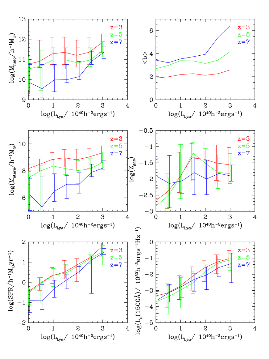
Figure 7: Model predictions for a range of physical properties of Ly$\alpha$ emitters plotted as a function of Ly$\alpha$ luminosity. In each panel the model predictions are shown for $z=3,5$ and 7. The lines show the median values of the respective properties (apart from panel (b) which shows the mean) and the error bars show the 10-90 percentile range. (a) The upper left panel shows the mass of the dark matter halo hosting the emitter. (b) The upper right panel shows the mean clustering bias. (c) The middlle left panel shows the stellar mass. (d) The middle right panel shows the metallicity of the cold gas. (e) The lower left panel shows the total star formation rate. (f) The lower right panel shows the UV continuum luminosity at a rest-frame wavelength of 1500Å.

5.1 Halo masses

The upper left panel of Fig.7 shows the masses of the dark matter halos hosting Ly$\alpha$ emitters. We see that at $z=3$, there is only a weak dependence of median halo mass on Ly$\alpha$ luminosity, while at $z=7$, the dependence is much stronger. At a given luminosity, the typical halo mass decreases with increasing redshift, with this trend being stronger at lower luminosities. As discussed in §5.5 below, the Ly$\alpha$ luminosity traces the instantaneous star formation rate (SFR) quite well in our model, but with a ratio which is $\sim 10$ times larger for bursting compared to quiescent galaxies, because of the difference in IMFs. There are two main reasons for the weak dependence of halo mass on Ly$\alpha$ luminosity at the lower redshifts: (a) the bursts introduce a large scatter into the relation between instantaneous SFR and object mass, especially at lower redshifts; (b) the shift from being dominated by bursts at high Ly$\alpha$ luminosities to being dominated by quiescent disks at lower luminosities flattens the trend of SFR with Ly$\alpha$ luminosity, which tends to hide the underlying trend of halo mass with SFR. Current Ly$\alpha$ surveys probe objects with luminosities $\sim 10^{42.5}h^{-2}{\rm erg\,s^{-1}}$ over the whole redshift range $z\sim 3-7$, for which the typical halo mass $\sim 10^{11}h^{-1}M_{\odot}$, declining by a factor $\sim 3$ from $z=3$ to $z=7$.

5.2 Clustering bias

The halo masses of LAEs can be constrained observationally from measurements of their clustering. Since the predicted halo masses for typical observed LAEs are larger than the characteristic halo mass at each redshift, we expect the LAEs to be more strongly clustered than the dark matter. We have used the halo masses predicted by the model to calculate the linear clustering bias $b$, which is expected to describe the clustering on large scales, using the formula of Sheth, Mo & Tormen (2001). We calculate a mean bias for objects in each range of luminosity. This mean bias is shown in the upper right panel of Fig.7. Over the luminosity range $L_{Ly\alpha}=10^{40}-10^{43}h^{-2}{\rm erg\,s^{-1}}$, our model predicts that the bias increases with redshift at fixed luminosity. At $z=3$, we predict $b\approx 2$ over this luminosity range, increasing only very slightly with luminosity. At $z=7$, the bias is predicted to vary much more strongly with luminosity, from $b\approx 3$ at $L_{Ly\alpha}=10^{40}h^{-2}{\rm erg\,s^{-1}}$ to $b\approx 6$ at $10^{43}h^{-2}{\rm erg\,s^{-1}}$. These predictions for the clustering of LAEs seem generally consistent with current observational constraints. The most reliable measurement of the clustering of LAEs to date is probably that of Ouchi et al. (2005), since their sample covers by far the largest comoving volume. For galaxies at $z=5.7$ with Ly$\alpha$ luminosities $\sim 10^{42}h^{-2}{\rm erg\,s^{-1}}$, they find a large-scale clustering bias $b=3.4\pm 1.8$. For the same redshift and luminosity, our model predicts $b\approx 4$, in excellent agreement with this measurement. At somewhat lower redshifts, $z\approx 4.8$, somewhat conflicting results have been obtained for the clustering (e.g. Ouchi et al, 2003; Shimasaku et al., 2003, 2004; Hamana et al. , 2004), however, these have been obtained from much smaller survey volumes. In particular, Shimasaku et al. (2004) measure very different clustering in their two approximately equal survey volumes at $z=4.8$, showing that the surveys used were not large enough to reliably measure the average clustering.

5.3 Stellar masses

The middle left panel of Fig.7 shows the predicted stellar masses of LAEs as a function of Ly$\alpha$ luminosity. The trends of stellar mass with luminosity and redshift are similar to those already discussed for the halo mass: the trend of stellar mass with luminosity steepens with increasing redshift, and the mass at a given luminosity decreases with increasing redshift. The reasons for the rather flat trend of stellar mass with Ly$\alpha$ luminosity at the lower redshifts are the same as those already given for the halo mass. For a luminosity $L_{Ly\alpha}=10^{42.5}h^{-2}{\rm erg\,s^{-1}}$, the median stellar mass is predicted to decrease from $\sim 10^{9}h^{-1}M_{\odot}$ at $z=3$ to $\sim 3\times 10^{7}h^{-1}M_{\odot}$ at $z=7$.

There have not yet been any observational estimates of the stellar masses of LAEs, but the values predicted by our model are rather lower than the stellar masses inferred observationally for some other classes of high-redshift galaxies. Shapley et al.  (2001) estimated stellar masses of Lyman-break galaxies at $z\sim 3$ from broad-band photometry, and found a median stellar mass $\sim 10^{10}h^{-1}M_{\odot}$ in a sample with median magnitude $R_{AB}\sim 24$ (similar results were also found by Papovich, Dickinson & Ferguson 2001). In contrast, typical observed LAEs at $z\sim 3$ with $L_{Ly\alpha}\sim 10^{42}h^{-2}{\rm erg\,s^{-1}}$ are predicted by our model to have stellar masses $\sim 10^{9}h^{-1}M_{\odot}$. The difference could be explained by a combination of two effects: (a) The LAEs at $z\sim 3$ with $L_{Ly\alpha}\sim 10^{42}h^{-2}{\rm erg\,s^{-1}}$ typically have fainter continuum magnitudes (by 1-2 mag) than the Shapley et al.  LBGs. (b) The photometric estimates of the stellar masses of LBGs depend strongly on the IMF assumed, because the mass-to-light ratio of a stellar population is very sensitive to the IMF; Shapley et al.  assumed a Salpeter IMF, but if instead they had assumed a top-heavy IMF as in starbursts in our model, then they might have derived lower masses.

The issue of how photometric estimates of the stellar masses of high-redshift galaxies depend on the assumed IMF is an important one, but is also complicated, because these estimates involve fitting multi-parameter models (varying age, star formation history, metallicity and dust extinction) to multi-band photometric data, in order to estimate the mass-to-light ratio of the stellar population. Most such studies have simply assumed a Salpeter IMF. Papovich, Dickinson & Ferguson (2001) considered the effects on photometric mass estimates of varying the lower mass limit on the IMF, but did not consider IMF slopes different from the solar neighbourhood value. We plan to address this issue in more detail in a future paper.

5.4 Metallicities

The middle right panel of Fig.7 shows the metallicity of the cold gas in LAEs as a function of Ly$\alpha$ luminosity. We see that in most cases, the gas metallicity is appreciable, $\sim 10^{-2}$ (i.e. comparable to solar), even at high redshifts. This reflects the fact that galaxies are able to self-enrich to metallicities $\sim Z_{\odot}$ even when the mean metallicity of all baryons in the universe is much lower than this. In our model, the quiescent galaxies are predicted to show a well-defined trend of metallicity increasing with luminosity (as already found for $z=0$ galaxies by Cole et al. 2000), which produces the decline in metallicity at low luminosities seen in Fig.7 for $z=3$ and $z=5$. However, the bursts show a more complicated behaviour, with the median metallicity being flat or even non-monotonic with luminosity, which is reflected in the behaviour seen in Fig.7 for $z=7$ and for higher luminosities at $z=3$ and $z=5$.

5.5 Star formation rates

The lower left panel of Fig.7 shows the instantaneous star formation rates in LAEs as a function of Ly$\alpha$ luminosity. The star formation rates include both the quiescent star formation in galactic disks and the contribution of any ongoing starbursts. If we look at either quiescent galaxies or bursts separately, then we find a nearly linear relation $SFR\propto L_{Ly\alpha}$, but with a proportionality constant which is $\sim 10$ times larger for the quiescent galaxies, because of the difference in IMFs. For a galaxy which has been forming stars at a contant rate for $10^{8}{\rm yr}$, we predict a relation $L_{Ly\alpha}=(1.1,12)\times 10^{42}{\rm erg\,s^{-1}}f_{\rm esc}(SFR/M_{\odot}{\rm yr}^{-1})$ for the Kennicutt and $x=0$ IMFs respectively (for solar metallicity), and quiescent and bursting galaxies in our model separately lie quite close to one or other relation. In Fig.7 we see a shallower relation than $SFR\propto L_{Ly\alpha}$ in some cases, which results from a gradual transition from being dominated by bursts at high luminosities to being dominated by quiescently star-forming galaxies at low luminosities. For LAEs with luminosities $\sim 10^{42.5}h^{-2}{\rm erg\,s^{-1}}$ (which are dominated by bursts), our model predicts SFRs $\sim 10h^{-1}M_{\odot}{\rm yr}^{-1}$. We note that comparing the SFRs predicted by our model with published values estimated from observational data is not straightforward, because different authors (a) assume different values for the Ly$\alpha$ escape fraction (often taking $f_{\rm esc}=1$), and (b) assume different IMFs (typically using a Salpeter IMF).

5.6 UV continuum luminosities

The lower right panel of Fig.7 shows the UV continuum luminosity $L_{\nu}(1500\AA)$ at a fixed rest-frame wavelength of 1500Å as a function of Ly$\alpha$ luminosity. This plot contains similar information to Fig.5, but now, for convenience, in terms of luminosities, and at a fixed rest-frame wavelength in the UV. The predicted relation between UV and Ly$\alpha$ luminosities is roughly linear. This is what one would expect if one had a universal IMF and no dust attenuation, since both the UV and Ly$\alpha$ luminosities are driven by recent star formation. For a galaxy which has been forming stars at a contant rate for $10^{8}{\rm yr}$, we predict an unattenuated relation $L_{\nu}(1500\AA)=(0.98,3.8)\times 10^{28}{\rm erg\,s^{-1}}{\rm Hz}^{-1}(SFR/M_{\odot}{\rm yr}^{-1})$ for the Kennicutt and $x=0$ IMFs respectively, for solar metallicity. However, dust extinction is predicted to have a large effect on UV luminosities in our model, reducing them by a factor $\sim 10$ in the brighter objects. The average UV extinction in the models increases with luminosity in both bursts and quiescent galaxies, and is also larger in quiescent than bursting objects (at a given SFR). The unattenuated UV/Ly$\alpha$ luminosity ratio is also predicted to decrease by a factor 3 going from quiescent objects at low luminosity to bursts at high luminosity as a result of the change in the IMF. These effects all combine to leave a relation between UV and Ly$\alpha$ luminosities which is shifted but still roughly linear.

The UV and Ly$\alpha$ luminosities are both used in estimating star formation rates for observed high-redshift galaxies. However, both suffer from the drawback that they are affected by large but uncertain dust attenuation factors. In the model presented here, the dust attenuation is larger by a factor $\sim 10$ for the Ly$\alpha$ than for the UV luminosity, so by that criterion, the UV luminosity should be a more reliable quantitative star formation indicator. However, we caution that the Ly$\alpha$ attenuation factor $f_{\rm esc}$ which we use was not obtained from a detailed radiative transfer calculation, unlike the UV dust extinction.

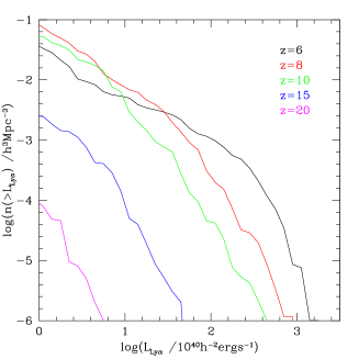
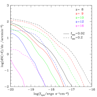
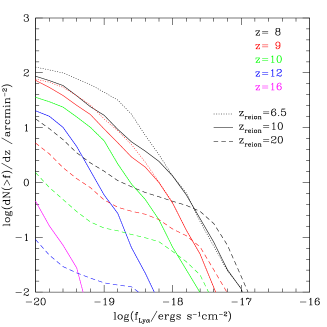
Figure 8: Predictions for the number of Ly$\alpha$ emitters at very high redshifts. (a) The upper panel shows the evolution of the cumulative Ly$\alpha$ luminosity function at $6\leq z\leq 20$, for our standard model, with reionization redshift $z_{\rm reion}=10$ and Ly$\alpha$ escape fraction $f_{\rm esc}=0.02$. (b) The middle panel shows the predicted number counts per unit redshift interval per unit solid angle as a cumulative function of the Ly$\alpha$ flux, for $z_{\rm reion}=10$. Results are shown for two different escape fractions, our standard value $f_{\rm esc}=0.02$ (solid lines) and a larger value $f_{\rm esc}=0.2$ (dashed lines). We show number counts for selected redshifts falling within either the J,H or K atmospheric transmission windows, with different redshifts in different colours. (c) The lower panel shows the cumulative number counts as in (b), for our standard $f_{\rm esc}=0.02$, and three different reionization redshifts, $z_{\rm reion}=6.5$ (dotted lines), 10 (solid lines) and 20 (dashed lines); where the dotted lines are not visible, they coincide with the solid lines. The number counts do not include attenuation by the IGM.

6 The abundance of Ly$\alpha$ emitters at $z>7$

Paper I presented predictions for the abundance of Ly$\alpha$ emitters as a function of flux for the redshift range $2\la z\la 7$ which is accessible from observations at optical wavelengths. The highest redshift at which LAEs have been found in surveys up to now is $z=6.6$. At even higher redshifts, the Ly$\alpha$ line moves into the near-IR as seen from the Earth. Therefore, searching for LAEs at $z\ga 7$ requires observing in the near-IR, which is technically challenging. Several such searches are underway (e.g. Willis & Courbin, 2005; Stark & Ellis, 2005), and others will start in the near future (e.g. Horton et al., 2004). Therefore in this section we present some predictions for the number of LAEs which should be found in near-IR searches, at redshifts $7\la z\la 20$. Barton et al. (2004) have previously made predictions for the number of LAEs at $z\approx 8$ based on a numerical simulation, but assumed a 100% escape fraction for Ly$\alpha$ photons (i.e. $f_{\rm esc}=1$). Thommes & Meisenheimer (2005) have also made predictions for $z>7$, but for a phenomenological model not based on CDM.

The upper panel of Fig.8 shows what our standard model, with reionization redshift $z_{\rm reion}=10$ and Ly$\alpha$ escape fraction $f_{\rm esc}=0.02$, predicts for the evolution of the luminosity function of LAEs at $6\leq z\leq 20$. We see that the luminosity function declines significantly at the bright end from $z\sim 6$ to $z\sim 10$, and then declines with redshift very rapidly at all luminosities at $z\ga 10$. This decline is driven by the reduction in star formation with increasing redshift, which results from the build-up of cosmic structure over time.

The middle and lower panels of Fig.8 show the predicted number counts per unit solid angle per unit redshift as a cumulative function of the Ly$\alpha$ flux. These predictions do not include the attenuation of the Ly$\alpha$ flux by neutral gas in the intervening IGM, as we discuss below. We show predictions for redshifts $z=8,9,10,12$ and $16$, chosen such that the Ly$\alpha$ line falls within either the J, H or K atmospheric window. (The J, H and K atmospheric windows cover the wavelength ranges 1.08-1.35, 1.51-1.80 and 1.97-2.38 $\mu$m respectively, corresponding to Ly$\alpha$ redshift ranges $z=7.9-10.1$, $11.4-13.8$ and $15.2-18.6$.) Ground-based searches in the near-IR are likely to concentrate on these atmospheric windows, because the atmospheric opacity at other near-IR wavelengths is extremely high. We have already shown predicted angular sizes for these galaxies in Fig.6(b).

The middle panel of Fig.8 shows how the predicted number counts depend on the assumed Ly$\alpha$ escape fraction $f_{\rm esc}$. We show results for our standard value of the reionization redshift $z_{\rm reion}=10$, but for two values of $f_{\rm esc}$, 0.02 (our standard value) and 0.2. We recall that the value of $f_{\rm esc}$ was originally chosen in order to match the observed counts at $z\sim 3$, and turns out to provide a good match to observations over the whole range $3<z<6.6$. At higher redshifts, no empirical calibration of $f_{\rm esc}$ is available. Since we do not have a detailed physical model for $f_{\rm esc}$, we cannot exclude the possibility that the value at very high redshifts is different from the value at lower redshifts. As might be expected, the number counts at a given flux are quite sensitive to the value of $f_{\rm esc}$. Predicted counts for other values of $f_{\rm esc}$ than those shown in Fig.8 can easily be obtained by scaling the curves in the horizontal direction with $f_{\rm esc}$, since the flux from each galaxy is proportional to $f_{\rm esc}$.

The lower panel of Fig.8 shows how the predicted number counts depend on the assumed reionization redshift $z_{\rm reion}$. As was discussed in Section 2, observations of Gunn-Peterson absorption troughs in QSO spectra suggest that the IGM became fully reionized at $z\sim 6$ (Becker et al. , 2001), while the WMAP measurement of the polarization of the microwave background implies that the IGM has been mostly reionized since $z\sim 20$ (Kogut et al. , 2003). We therefore show predictions for $z_{\rm reion}=6.5$ and 20, in addition to our standard value $z_{\rm reion}=10$. In all three cases we assume $f_{\rm esc}=0.02$. In our model, reionization is assumed to affect galaxy formation in the following way: the IGM is assumed to be instantaneously reionized and reheated at $z=z_{\rm reion}$, and at $z<z_{\rm reion}$, the thermal pressure of the IGM is assumed to prevent gas collapsing in all dark halos with circular velocities $V_{c}<60{\rm km\,s^{-1}}$. This simple behaviour is an approximation to what was found in more detailed calculations by Benson et al. (2002). The dependence of the number counts on $z_{\rm reion}$ shown in Fig.8 results entirely from this effect of reionization on galaxy formation, since we ignore the IGM opacity here. For $z>z_{\rm reion}$, all models look identical to the case in which the IGM never reionized, but for $z<z_{\rm reion}$, the number counts are suppressed relative to the no-reionization case. We see that the predicted counts for the redshift ranges and fluxes shown in Fig.8 differ only slightly for $z_{\rm reion}=6.5$ and $z_{\rm reion}=10$, but for $z_{\rm reion}=20$, the predicted counts are much lower, except for the bright counts at $z\sim 8-10$.

However, as noted earlier, there is an important caveat to our results: our model includes the attenuation of the stellar continuum light from galaxies due to Ly$\alpha$ scattering and Lyc absorption by atomic hydrogen in the intervening IGM, but we do not include any attenuation of the flux in the Ly$\alpha$ line due to Ly$\alpha$ scattering in the IGM. At $z>z_{\rm reion}$, when the IGM is completely neutral, this attenuation of the Ly$\alpha$ line flux could potentially be very large, which would greatly decrease the number counts at a given flux. IGM attenuation will therefore produce a trend in the number counts with $z_{\rm reion}$ in the opposite sense to the feedback of reionization on galaxy formation: at $z<z_{\rm reion}$, the feedback effect tends to suppress the counts, but the IGM attenuation will be removed, which will increase the counts relative to a model in which the IGM is still neutral at that redshift.

The amount of attenuation of the Ly$\alpha$ line by the IGM before reionization is theoretically very uncertain. Miralda-Escude (1998) showed that for a galaxy at high redshift embedded in a neutral IGM moving with the Hubble flow, emitting a Ly$\alpha$ line centred at its rest-frame wavelength in the frame of the galaxy, scattering by atomic hydrogen in the IGM would suppress the blue wing of the Ly$\alpha$ line completely (reducing the line flux by a factor 2), and also partly suppress the red wing due to the Ly$\alpha$ damping wings (reducing the line flux even more). However, Madau & Rees (2000) and Haiman (2002) showed that this attenuation of the line flux could be greatly reduced due to the galaxy photo-ionizing the IGM around it. A more detailed theoretical analysis of the attenuation has been made by Santos (2004), who includes the following effects: (i) the intrinsic width of the Ly$\alpha$ line emitted by the galaxy, and the fact it may be redshifted in the galaxy rest-frame due to scattering in a galactic wind; (ii) the non-uniform density profile of the IGM around the galaxy and the departure of the velocity field from the Hubble flow, due to cosmological infall onto the galaxy; (iii) collisional ionization of the gas within the galaxy halo, photo-ionization of the surrounding IGM by the stellar population, and clearing of bubbles in the IGM by galactic winds. Santos finds that a very wide range of attenuation factors is possible in plausible models, but that if the Ly$\alpha$ emission is redshifted in the rest-frame of the galaxy (as is observed to be the case in Lyman-break galaxies at $z\sim 3$), the amount of attenuation is greatly reduced. The effects on the attenuation of Ly$\alpha$ of clustering of galaxies and clumping of the IGM have been investigated by Furlanetto et al. (2004) Gnedin & Prada (2004), and Wyithe & Loeb (2005); they find that these effects can also significantly reduce the amount of attenuation. In summary, for LAEs at $z>z_{\rm reion}$, the Ly$\alpha$ flux is likely to be significantly attenuated by the IGM, but the amount of attenuation is currently uncertain. We plan to investigate this in more detail in a future paper.

An unsuccessful search for LAEs at $z=8.8$ has been carried out by Willis & Courbin (2005), who place an upper limit $n\la 3\times 10^{-3}h^{3}{\rm Mpc}^{-3}$ on sources with $L_{Ly\alpha}>10^{43}h^{-2}{\rm erg\,s^{-1}}$. This limit on the number density is more than 4 orders of magnitude higher than the prediction for our standard model shown in Fig.8(a). Willis et al.  (2005) and Stark & Ellis (2005) are carrying out surveys for $z\sim 9$ LAEs which will probe to lower luminosities by using gravitational lensing by foreground clusters. In the near future, the DAzLE instrument (Horton et al., 2004) on the VLT will begin searches for LAEs at $z>7$. It is planned to search for Ly$\alpha$ at $z\approx 7.7$ in the first phase, and $z\approx 8.7$ in the second phase, in each case over a redshift window $\Delta z\approx 0.01$; ultimately it may be possible to reach $z\approx 14$ with the instrument. DAzLE will cover an area of $\Delta\Omega=47\,{\rm arcmin}^{2}$ in a single exposure, and is projected to reach a $5\sigma$ flux limit of $f=2\times 10^{-18}{\rm erg\,cm^{-2}s^{-1}}$ in a 10 hour integration. We can use our model to predict how many objects DAzLE should see in a single 10 hour exposure in each of the redshift ranges. For our standard model with $z_{\rm reion}=10$ and $f_{\rm esc}=0.02$, we predict the number of sources per unit redshift per unit solid angle above flux $f=2\times 10^{-18}{\rm erg\,cm^{-2}s^{-1}}$ to be $d^{2}N(>f)/d\Omega dz=(0.58,0.13)\,{\rm arcmin}^{-2}$ at $z=(7.7,8.7)$ respectively, which for the specified $\Delta z$ and $\Delta\Omega$ corresponds to an average of 0.3 and 0.06 objects per field at $z=7.7$ and $z=8.7$ respectively. Therefore we expect that DAzLE will need to observe many separate fields to find a significant number of high-z Ly$\alpha$ emitters.

7 Conclusions

In this paper, we have used a detailed semi-analytical model of galaxy formation based on the $\Lambda$CDM cosmology to predict the properties of star-forming Ly$\alpha$-emitting galaxies over the redshift range $0\leq z\leq 20$. All except one of the parameters of the model were chosen without reference to the observed properties of Ly$\alpha$ emitters, having instead been chosen in previous work (Cole et al., 2000; Baugh et al., 2005) to match properties such as the UV, optical and IR luminosities, sizes, morphological types, gas fractions and metallicities of galaxies at low and high redshift. As shown in Baugh et al. (2005), our current model, which incorporates a top-heavy IMF for stars formed in bursts triggered by galaxy mergers, provides a good match to the optical and far-IR luminosity functions in the local universe, the far-UV luminosity function of Lyman-break galaxies at $z\sim 3$, and the number counts and redshifts of sub-mm galaxies. Our assumption of a top-heavy IMF in bursts receives support from studies of the metallicities of elliptical galaxies and intracluster gas (Nagashima et al., 2005a, b). The one free parameter we had in the comparison of our model with observational data on Ly$\alpha$ emitters (LAEs) was the fraction $f_{\rm esc}$ of Ly$\alpha$ photons which escape from a galaxy. For simplicity, we have assumed that $f_{\rm esc}$ is a constant, irrespective of other galaxy properties. In our previous paper on LAEs (Le Delliou et al., 2005), we found that $f_{\rm esc}=0.02$ reproduced the abundance of faint LAEs at $z\sim 3$, and we used the same value in the present paper.

In Le Delliou et al. (2005), we presented model predictions for the number counts of LAEs as a function of Ly$\alpha$ flux for the redshift range $2\leq z\leq 6$, but made only a very limited comparison with observational data, comparing only with the total counts at the limiting fluxes for different surveys. In this paper, we have made a much more detailed comparison of the model with observations, comparing predicted and observed Ly$\alpha$ luminosity functions over the range $3\leq z\leq 7$. The most important result of this paper is that, with our very simple assumption of a constant Ly$\alpha$ escape fraction, the model reproduces the observed luminosity functions, both in shape and in the evolution with redshift.

We have also compared the predictions of our model with other observed properties of LAEs. We have made a comparison of predicted and observed Ly$\alpha$ equivalent widths (EWs). We find that the typical predicted EWs are similar to those found in observational surveys, and that the predicted distribution of EWs at a given Ly$\alpha$ flux is very broad once we include the effect of dust extinction, with a peak at 0 and a tail to large values. If we select galaxies in the model according to their continuum magnitudes rather than their Ly$\alpha$ fluxes, then we predict a distribution of EWs which is similar to what has been found observationally for Lyman-break galaxies at $z\sim 3$, when we restrict the comparison to galaxies where Ly$\alpha$ is seen in emission. We have compared predicted and observed broad-band magnitudes (corresponding to rest-frame UV luminosities) for galaxies selected by their Ly$\alpha$ fluxes, and find mostly good agreement. We have also compared the predicted sizes of LAEs with the limited existing observational data, and find reasonable consistency for the stellar half-light radii.

We have also used our model to try to better understand the nature of the objects selected in Ly$\alpha$ emission-line surveys, and how they relate to other classes of high-redshift galaxies. We have made predictions for the dark halo and stellar masses, the star formation rates and the gas metallicities for LAEs at different redshifts, properties which are physically fundamental, but for which we do not yet have direct observational measurements. The predicted halo masses imply values of the clustering bias which seem quite consistent with existing measurements of the large-scale clustering of LAEs. Better observational characterization of the clustering of LAEs at different redshifts would provide a very important test of our model.

Finally, we have presented predictions for how many Ly$\alpha$ emitters should be seen at $z>7$, a redshift range for which no LAEs have yet been found, but which is now opening up for observational study, thanks to advances in near-IR instrumentation. Detection of LAEs in this redshift range would be very exciting both for probing the early stages of galaxy formation and the epoch of reionization. A problem for making predictions for LAEs at $z>7$ is that the redshift at which the IGM reionized is uncertain, being observationally constrained to be in the range $6.5\la z_{\rm reion}\la 20$. This affects predictions for galaxies seen at $z>z_{\rm reion}$, since the Ly$\alpha$ flux is expected to be significantly attenuated by propagation through a neutral IGM, but by an uncertain amount which depends on many factors. We have made detailed predictions for how many objects could be seen using the DAzLE instrument, which begins operation soon, at $z\approx 7.7$ and $z\approx 8.7$. We find that, even if the attenuation by the IGM is modest at these redshifts, then finding LAEs with DAzLE will require observation of a large number of fields.

The most important theoretical limitations of our present work are that it does not incorporate a detailed physical model for the escape of Ly$\alpha$ photons from galaxies, and that we do not include a treatment of the attenuation of Ly$\alpha$ fluxes by the IGM prior to reionization. We plan to address these issues in future papers.

References

- Ahn (2004) Ahn, S.-H., 2004, ApJ, 601, L25
- Ajiki et al. (2003) Ajiki, M., Taniguchi, Y., Fujita, S.S., Shioya, Y., Nagao, T., Murayama, T., Yamada, S., Umeda, K., & Komiyama, Y., 2003, AJ, 126, 2091
- Barton et al. (2004) Barton, E.J., Dave, R., Smith, J-D.T., Papovich, C. Hernquist, L. Springel, V., 2004, ApJ 604, L1
- Baugh et al. (2005) Baugh C.M., Lacey C.G., Frenk C.S., Granato G.L., Silva L., Bressan A., Benson A.J., & Cole S., 2005, MNRAS, 356, 1191
- Becker et al. (2001) Becker R.H., Fan, X., White, R.L., Strauss, M.A., Narayanan, V.K., Lupton, R.H., Gunn, J.E., Annis, J., Bahcall, N.A., Brinkmann, J., and 20 coauthors, 2001, AJ, 122, 2850.
- Benson et al. (2002) Benson, A.J., Lacey, C.G., Frenk, C.S., Baugh, C.M., Cole, S., 2002, MNRAS 333, 156
- Benson et al. (2003) Benson, A.J., Bower, R.G., Frenk, C.S., Lacey, C.G., Baugh, C.M., Cole, S., 2003, ApJ 599, 38
- Bower et al. (2004) Bower, R. G., Morris, S. L., Bacon, R., Wilman, R. J., Sullivan, M., Chapman, S., Davies, R. L., de Zeeuw, P. T., Emsellem, E., 2004, MNRAS, 351, 63
- Cantalupo et al. (2005) Cantalupo, S., Porciani, C., Lilly, S., Miniati, F., 2005, ApJ 628, 61
- Charlot & Fall (1991) Charlot, S., Fall, S.M., 1991, ApJ 378, 471
- Charlot & Fall (1993) Charlot, S., Fall, S.M., 1993, ApJ 415, 580
- Cole et al. (2000) Cole S., Lacey C.G., Baugh C.M., Frenk C.S., 2000, MNRAS, 319, 168.
- Cowie & Hu (1998) Cowie L.L., Hu E.M., 1998, AJ, 115, 1319.
- Dawson et al. (2004) Dawson, S., Rhoads, J.E., Malhotra, S., Stern, D., Dey, A., Spinrad, H., Jannuzi, B.T., Wang, J., Landes, E., 2004, ApJ 617, 707
- Ellis et al. (2001) Ellis, R., Santos, M.R., Kneib, J.-P., Kuijken, K., 2001, ApJ, 560, L119
- Fardal et al. (2001) Fardal, M.A., Katz, N., Gardner, J., Hernquist, L., Weinberg, D.H., Dave, R., 2001, ApJ 562, 605
- Furlanetto et al. (2004) Furlanetto, S.R., Hernquist, L., Zaldarriaga, M., 2004, MNRAS 354, 695
- Furlanetto et al. (2005) Furlanetto, S.R., Schaye, J., Springel, V., Hernquist, L., 2005, ApJ, 622, 7
- Gnedin & Prada (2004) Gnedin, N.Y., Prada, F., 2004, ApJ 608, L77
- Granato et al. (2000) Granato, G.L., Lacey C.G., Silva, L., Bressan, A., Baugh C.M., Cole S., Frenk C.S., 2000, ApJ 542, 710
- Haiman (2002) Haiman, Z., 2002, ApJ 576, L1
- Haiman & Spaans (1999) Haiman, Z., Spaans, M., 1999, ApJ, 518, 138
- Haiman, Spaans & Quataert (2000) Haiman, Z., Spaans, M., Quataert, E., 2000, ApJ, 537, L5
- Hamana et al. (2004) Hamana, T., Ouchi, M., Shimasaku, K., Kayo, I., Suto, Y., 2004, MNRAS 347, 813
- Hansen & Oh (2005) Hansen, M., Oh, S.P., 2005, submitted to MNRAS (astro-ph/0507586)
- Hogan & Weymann (1987) Hogan, C.J., Weymann, R.J, 1987, MNRAS, 225, 1P
- Horton et al. (2004) Horton, A., Parry, I.R., Bland-Hawthorn, J.. Cianci, S., King, D, McMahon, R., Medlen, S., 2004, Proceedings of SPIE Vol. 5492, “Ground-based Instrumentation for Astronomy”, 1022 (astro-ph/0409080)
- Hu, Cowie & McMahon (1998) Hu E.M., Cowie L.L., McMahon R.G., 1998, ApJ, 502, L99.
- Hu et al. (2004) Hu, E. M., Cowie, L. L., Capak, P., McMahon, R. G., Hayashino, T., & Komiyama, 2004, AJ, 127, 563
- Kennicutt (1983) Kennicutt R.C., 1983, ApJ, 272, 54.
- Kogut et al. (2003) Kogut A., et al. (the WMAP team), 2003, ApJS, 148, 161.
- Kudritzki et al. (2000) Kudritzki, R.-P., Mendez, R. H., Feldmeier, J. J., Ciardullo, R., Jacoby, G. H., Freeman, K. C., Arnaboldi, M., Capaccioli, M., Gerhard, O., Ford, H. C., 2000ApJ, 536, 19
- Kunth et al. (1998) Kunth, D., Mas-Hesse, J.M., Terlevich, E., Terlevich, R., Lequeux, J., Fall, S.M., 1998, A&A, 334, 11
- Le Delliou et al. (2005) Le Delliou, M., Lacey, C., Baugh, C.M., Guiderdoni, B., Bacon, R., Courtois, H., Sousbie, T., & Morris, S.L., 2005, MNRAS, 357, L11 (Paper I)
- Madau (1995) Madau, P., 1995, ApJ 441, 18
- Madau & Rees (2000) Madau, P., Rees, M.J., 1995, ApJ 542, L69
- Maier et al. (2003) Maier, C., Meisenheimer, K., Thommes, E., Hippelein, H., Roser, H. J., Fried, J., von Kuhlmann, B., Phleps, S., Wolf, C., 2003, A&A, 402, 79 (CADIS)
- Mas-Hesse et al. (2003) Mas-Hesse, J.M., Kunth, D., Tenorio-Tagle, G., Leitherer, C., Terlevich, R., Terlevich, E., 2003, ApJ 598, 858
- Matsuda et al. (2004) Matsuda, Y., Yamada, T., Hayashino, T., Tamura, H., Yamauchi, R., Ajiki, M., Fujita, S.S., Murayama, T., Nagao, T., Ohta, K., and 5 coauthors, 2004, AJ 128, 569
- McCarthy et al. (1987) McCarthy, P.J., Spinrad, H., Djorgovski, S., Strauss, M.A., van Breugel, W., Liebert, J., 1987, ApJ 319, L39
- Miralda-Escude (1998) Miralda-Escude, J., 1998, ApJ 501, 15
- Nagashima et al. (2005a) Nagashima, M., Lacey, C.G., Baugh, C.M., Frenk, C.S., Cole, S., 2005, MNRAS 358, 1247
- Nagashima et al. (2005b) Nagashima, M., Lacey, C.G., Okamoto, T., Baugh, C.M., Frenk, C.S., Cole, S., 2005, MNRAS, 363, L31
- Neufeld (1991) Neufeld, D.A., 1991, ApJ 370, L85
- Osterbrock (1989) Osterbrock D.E., 1989, Astrophysics of Gaseous Nebulae and Active Galactic Nuclei, University Science Books
- Ouchi et al (2003) Ouchi, M., Shimazaku, K., Furusawa, H., Miyasaki, M., Doi, M., Hamabe, M., Hayashino, T., Kimura, M., Kodaira, K., & Komiyama, Y., and 10 coauthors, 2003, ApJ, 582, 60
- Ouchi et al. (2005) Ouchi, M., Shimazaku, K., Akiyama, M., Sekiguchi, K., Furusawa, H., Okamura, S., Kashikawa, N., Iye, M., Kodama, T., Saito, T., and 7 coauthors, 2005, ApJ 620, L1
- Papovich, Dickinson & Ferguson (2001) Papovich, C., Dickinson, M., Ferguson, H.C., 2001, ApJ 559, 620
- Partridge & Peebles (1967) Partridge, R.B., Peebles, P.J.E., 1967, ApJ, 147, 868.
- Pascarelle, Windhorst & Keel (1998) Pascarelle, S.M., Windhorst, R.A., Keel, W.C., 1998, AJ 116, 2659
- Pettini et al. (2001) Pettini M., Steidel C.C., Adelberger K.L., Dickinson M., Giavalisco M., 2001, ApJ, 528, 96.
- Rhoads et al. (2003) Rhoads, J.E., Dey, A., Malhotra, S., Stern, D., Spinrad, H., Jannuzi, B.T., Dawson, S., Brown, M.J.I., Landes, E., 2003, AJ, 125, 1006 (LALA)
- Santos (2004) Santos, M.R., 2004, MNRAS 349, 1137
- Santos et al. (2004) Santos, M.R., Ellis, R.S., Kneib, J.-P., Richard, J., Kuijken, K., 2004, ApJ 606, 683
- Shapley et al. (2001) Shapley, A.E., Steidel, C.C., Adelberger, K.L., Dickinson, M., Giavalisco, M. Pettini, M., 2001, ApJ 562, 95
- Shapley et al. (2003) Shapley, A.E., Steidel, C.C., Pettini, M., Adelberger, K.L., 2003, ApJ 588, 65
- Sheth, Mo & Tormen (2001) Sheth, R.H., Mo, H.J., Tormen, G., 2001, MNRAS 323, 1
- Shimasaku et al. (2003) Shimasaku, K., Ouchi, M., Okamura, S., Kashikawa, N., Doi, M., Furusawa, H., Hamabe, M., Hayashino, T., Kawabata, K., Kimura, M., and 15 coauthors, 2003, ApJ, 586, L11
- Shimasaku et al. (2004) Shimasaku, K., Hayashino, T., Matsuda, Y., Ouchi, M., Ohta, K., Okamura, S., Tamura, H., Yamada, T., Yamauchi, R., 2004, ApJ 605, L93
- Stanway et al. (2004) Stanway, E.R., Bunker, A.J., McMahon, R.G., Ellis, R.S., Treu, T., McCarthy, P.J., 2004, ApJ, 607, 704
- Stark & Ellis (2005) Stark, D.P., Ellis, R.S., 2005, submitted to New Astronomy (astro-ph/0508123)
- Steidel et al. (2000) Steidel, C.C., Adelberger, K.L., Shapley, A.E, Pettini, M., Dickinson, M., Giavalisco, M., 2000, ApJ, 532, 170
- Taniguchi et al. (2005) Taniguchi, Y., Ajiki, M., Nagao, T., Shioya, Y., Kashikawa, N., Kodaira, K., Kaifu, N., and 32 coauthors, 2005, PASJ, 57, 165
- Tenorio-Tagle et al. (1999) Tenorio-Tagle, G., Silich, S.A., Kunth, D., Terlevich, E., Terlevich, R., 1999, MNRAS 309, 332
- Thommes & Meisenheimer (2005) Thommes, E., Meisenheimer, K, 2005, A&A 430, 877
- Tran et al. (2004) Tran, K.-V., Lilly, S.J., Crampton, D., & Brodwin, M., 2004, ApJ, 612, L89
- Willis & Courbin (2005) Willis, J.P., Courbin, F., 2005, MNRAS 357, 1348.
- Willis et al. (2005) Willis, J.P., Courbin, F., Kneib, J.-P., Minniti, D., 2005, submitted to New Astronomy (astro-ph/0509600)
- Wyithe & Loeb (2005) Wyithe, J.S.B., Loeb, A., 2005, ApJ 625, 1