Cosmological structure formation in a homogeneous dark energy background

There is now strong evidence that the current energy density of the Universe is dominated by dark energy with an equation of state $w<-1/3$, which is causing accelerated expansion. The build-up of structure within such Universes is subject to significant ongoing study, particularly through the spherical collapse model. This paper aims to review and consolidate progress for cosmologies in which the dark energy component remains homogeneous on the scales of the structures being modelled. The equations presented are designed to allow for dark energy with a general time-varying equation of state $w(a)$. In addition to reviewing previous work, a number of new results are introduced: A new fitting formula for the linear growth factor in constant $w$ cosmologies is given. A new formalism for determining the critical density for collapse is presented based on the initial curvature of the perturbation. The commonly used approximation to the critical density for collapse based on the linear growth factor is discussed for a general dark energy equation of state. Virialisation within such cosmologies is also considered, and the standard assumption that energy is conserved between turn-around and virialisation is questioned and limiting possiblities are presented.

1 Introduction

Analysis of the distance-redshift relation using high redshift Type Ia supernovae has led to the discovery that the expansion of the Universe is currently accelerating (Riess et al. 1998; Perlmutter et al. 1999). This suggests that the dominant contribution to the present-day energy budget is a component with equation of state $w<-1/3$, called “dark-energy”. Combining measurements of CMB fluctuations (de Bernardis et al. 2000; Lee et al. 2001; Halverson et al. 2002; Pearson et al. 2003; Scott et al. 2003; Hinshaw et al. 2003) with measurements of the clustering of present day galaxies (Percival et al. 2001; Tegmark et al. 2004a; Cole et al. 2005) has confirmed this requirement for dark energy (e.g. Efstathiou et al. 2002; Percival et al. 2002; Spergel et al. 2003; Tegmark et al. 2004b). These studies favour a flat Universe with $\Omega_{M}\simeq 0.3$, with the remaining contribution made up of dark energy.

The nature of the dark energy is the source of much debate. Perhaps the most straightforward candidate is a positive cosmological constant $\Lambda$ with equation of state parameter $w=-1$. This simple picture forms a special case in a broader class of models where the dark energy is the manifestation of a scalar field slowly rolling down its potential. In the limit of a completely flat potential, these models lead to $w=-1$ (Wetterich 1988; Peebles & Ratra 1988; Ratra & Peebles 1988). A subclass of quintessence models with constant $-1<w<-1/3$ was proposed by Caldwell, Dave & Steinhardt (1998a, b). Many other forms have been proposed for the shape of this potential, leading to an equation of state parameter that is dependent on the scale factor (see Peebles & Ratra 2003 for a review).

Given the plethora of models, many parameterisations have been introduced in order to observationally constrain $w(a)$ (see Johri 2004 for a review). However, there is obviously a limitation imposed by any parameterisation (Bassett, Corasaniti & Kunz 2004) and, in the present paper, we have tried to be as general as possible in the equations presented and discussed. In order to demonstrate the effects of the dark energy equation of state in numerical examples, we pay particular attention to the parameterisation of Jassal, Bagla & Padmanabhan (2004)

$$w(a)=w_{0}+w_{1}a(1-a).$$ (1)

The present day value of $w|_{a=1}=w_{0}$, and its derivative $dw(a)/da|_{a=1}=-w_{1}$ will serve to demonstrate the possible cosmological signatures of a wider class of models. We also consider models that assume $w(a)=w$ is constant. Qualitatively, many of the effects of general $w(a)$ models can be predicted by interpolating between models with constant $w$. In fact, for many models, by the lookback time by which $w(a)$ has evolved significantly from its present day value, the cosmological significance of $w(a)$ is greatly reduced (although see, for example, Maor et al. 2002). Obviously, this also signifies that an evolving $w(a)$ is harder to observationally constrain than constant $w$ (Kujat et al. 2002). If the dark energy equation of state only varies slowly with time, then observational predictions are well approximated by treating $w(a)=w$ as a constant (Wang et al. 2000), with

$$w\simeq\frac{\int\,da\,\Omega_{X}(a)w(a)}{\int\,da\,\Omega_{X}(a)},$$ (2)

where $\Omega_{X}$ is the dark energy density relative to the critical density (see also Dave, Caldwell & Steinhardt 2002).

The equation of state for the dark energy does not uniquely define the behaviour of this component. The formation of structure is also dependent on the sound speed of the dark energy which limits its clustering properties. In the original formalism for quintessence (Caldwell, Dave & Steinhardt 1998a, b), the dark energy component has a high sound speed which means that it can cluster on the largest scales, but does not cluster on the scales of galaxy clusters and below.

Consequently, the dark energy only affects the matter power spectrum (Ma et al. 1999), and the CMB anisotropies (Caldwell, Dave & Steinhardt 1998b) on very large scales. For the special case of a cosmological constant, $w=-1$, the clustering of the dark energy is not an issue as the energy density in perturbations always remains at the background level. Obviously, for $w\neq-1$, the clustering properties of the dark energy strongly affect the build-up of structure in the Universe. In particular for spherical perturbations, the linear growth rate, critical overdensity for collapse, and details of subsequent behaviour and virialisation are all dependent on this property. In this paper we follow the majority of current literature and only consider a non-clustering dark energy component. However, we do note that models in which the dark energy clusters on small scales are being discussed with increasing frequency (Hu & Scranton 2004; Nunes & Mota 2004; Hannestad 2005; Manera & Mota 2005; Maor & Lahav 2005).

In general, for the variables used in this paper, if no dependence is quoted for a given quantity (e.g. $\Omega_{M}$), it should be assumed to be calculated at present day. If instead explicit dependence is given (e.g. $\Omega_{M}(a)$), the quantity is assumed to vary with epoch. The exception to this rule is $w(a)$, where if no dependence on $a$ is given, we additionally assume that $w(a)=w$ is constant in time.

We start by reviewing the behaviour of different cosmological models, and the critical parameters that separate models with different properties (Section 2) as this can be related to the behaviour of spherical perturbations. We then calculate the linear growth factor (Section 3), the critical overdensity for collapse at present day (Section 4), and as a function of time (Section 5). This critical overdensity is then used to determine the mass function (Section 6) and the rate of structure growth (Section 7). Finally we consider the virialisation of perturbations, and the difficulties associated with these calculations in dark energy cosmologies (Section 8).

2 dynamics of cosmological models

It is assumed that the dark energy has an equation of state relating its pressure $p_{X}$ and density $\rho_{X}$ given by $p_{X}=w(a)\rho_{X}$. For general $w(a)$, the dynamical expansion of the Universe is specified by the Friedmann equation

$$E^{2}(a)=\frac{H^{2}(a)}{H_{0}^{2}}=\Omega_{M}a^{-3}+\Omega_{K}a^{-2}+\Omega_{X}a^{f(a)},$$ (3)

where $\Omega_{K}\equiv(1-\Omega_{M}-\Omega_{X})$ is the curvature constant, $H(a)\equiv\dot{a}/a$ is the Hubble parameter with present day value $H_{0}$. $f(a)$ is calculated by solving the conservation of energy equation for the dark energy $d(\rho_{X}a^{3})/da=-3p_{X}a^{2}$ (Caldwell, Dave & Steinhardt 1998b), giving $\rho_{X}\propto a^{f(a)}$, where

$$f(a)=\frac{-3}{\ln a}\int_{0}^{\ln a}[1+w(a^{\prime})]d\ln a^{\prime}.$$ (4)

For constant $w$, $f(a)=-3(1+w)$. For the parameterisation $w(a)=w_{0}+w_{1}a(1-a)$ of Jassal, Bagla & Padmanabhan (2004),

$$f(a)=-3(1+w_{0})+\frac{3w_{1}}{2\ln a}(1-a)^{2}.$$ (5)

The evolution of the matter density $\Omega_{M}(a)$ and dark energy density $\Omega_{X}(a)$ are given by

$$\Omega_{M}(a)=\frac{\Omega_{M}a^{-3}}{E^{2}(a)},\,\,\,\Omega_{X}(a)=\frac{\Omega_{X}a^{f(a)}}{E^{2}(a)}.$$ (6)

It is immediately apparent that the equation of state of the dark energy has a strong affect on the behaviour of these equations, even for models where $w(a)$ is constant. For example, for $w=-1/3$, the dark energy terms in Eq. 3 cancel, leaving a cosmological model with an expansion time history that behaves exactly as an open Universe with matter density $\Omega_{M}$, although the space-time geometry differs (e.g. review by Peebles & Ratra 2003). For $w<-1/3$, at late times the dark energy will dominate the dynamics of the expansion, with the epoch of transition from matter to dark energy domination dependent on $w$. Decreasing the equation of state $w$ from $-1/3$ smoothly interpolates between the open Universe model, cosmological constant ($\Lambda$ model) and extrapolates beyond.

The asymptotic behaviour (either forwards or backwards in time) of different cosmological models is delineated by models with so-called critical parameters. These separate cosmologies that predict future recollapse, expansion forever and models that do not start at a big-bang, but instead “loiter” at early times, asymptotically tending towards a stable solution such as Einstein’s static model for $\Lambda$ cosmologies. For these critical models, the zero points of $(da/dt)^{2}=E^{2}(a)a^{2}=0$ should occur at turning points of this equation. For constant $w$, differentiating Eq. 3, we see that the critical cosmologies should have $E^{2}(a)a^{2}=0$ when (Chiba, Takahashi & Sugiyama 2005)

$$a_{\rm turn}=\left[\frac{\Omega_{M}}{-(1+3w)\Omega_{X}}\right]^{\frac{-1}{3w}}.$$ (7)

Substituting this value of the scale factor back into Eq. 3 gives an equation for the critical parameters.

For $w=-1$, this reduces to the well known cubic equation (Glanfield 1966)

$$(\Omega_{M}+\Omega_{\Lambda}-1)^{3}=\frac{27}{4}\Omega_{M}^{2}\Omega_{\Lambda}$$ (8)

that can be solved analytically (Felten & Isaacman 1986). A detailed discussion of the behaviour of $\Lambda$ models is given by Moles (1991).

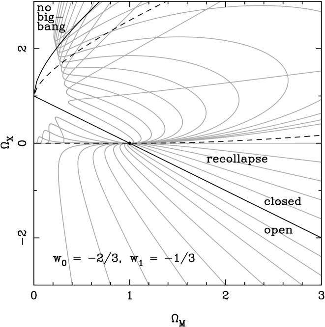
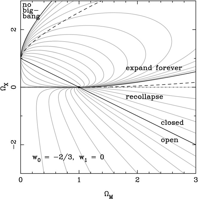
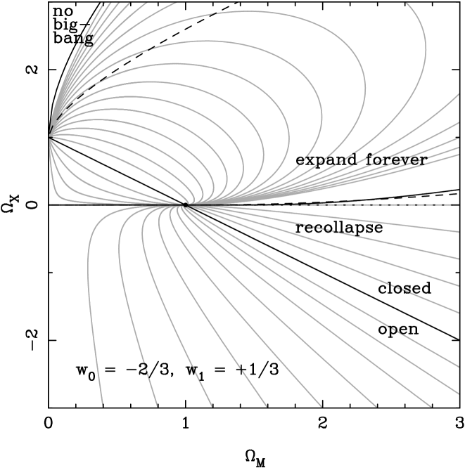
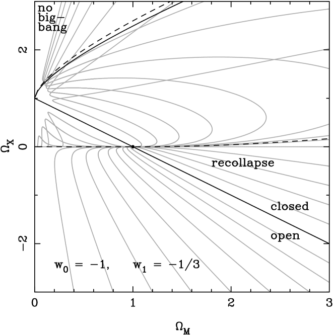
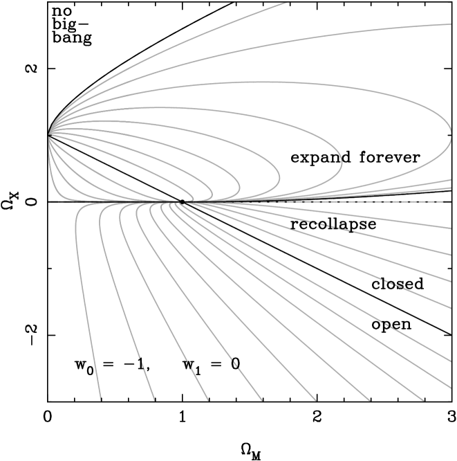
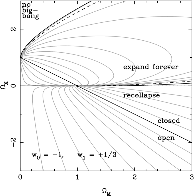
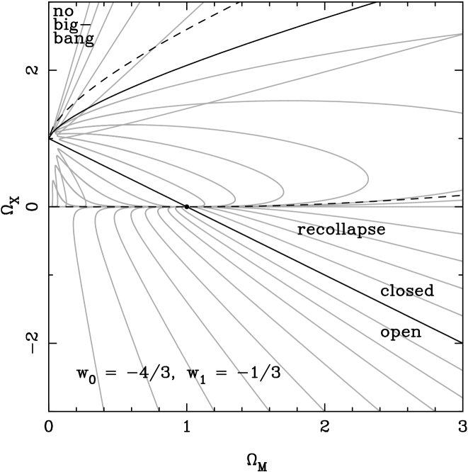
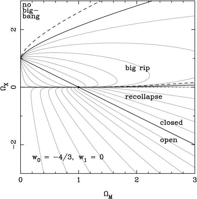
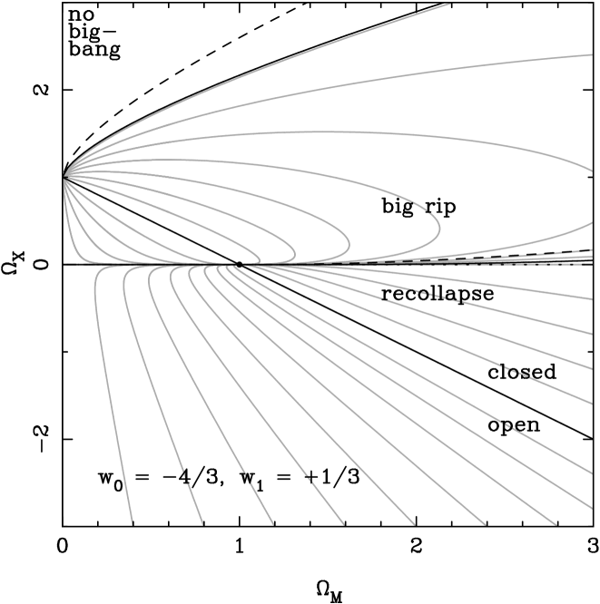
Figure 1: Plots showing the evolution of the matter and vacuum energy densities for a selection of cosmologies with different dark energy equation of state (grey lines). For cosmologies with $\Omega_{X}>0$, $a=1$ was fixed when the matter density and vacuum density were equal. The critical models that border the different types of evolution are shown by the black lines. Dashed lines in all plots show the critical models for $\Lambda$ cosmologies. The dotted line for $w_{1}\geq 0$ shows $\Omega_{X}=0$, to emphasis that recollapse can occur if $\Omega_{X}>0$ provided that $\Omega_{M}>>\Omega_{X}$.

For general $w(a)$, it is straightforward to numerically determine the critical parameters from Eq. 3 and its derivative. The different regions in ($\Omega_{M}$,$\Omega_{X}$) space are shown in Fig. 1 for $w_{0}=-4/3,-1,-2/3$ and $w_{1}=-1/3,0,1/3$ using the parameterisation of Eq. 1. Critical values of $\Omega_{M}$ and $\Omega_{X}$ at $a=1$ are shown by the solid black lines.

For comparison, in Fig. 1 we also plot various cosmological tracks (grey lines). For general $w(a)$ models, the cosmology is not uniquely specified by $\Omega_{M}(a)$ and $\Omega_{X}(a)$, as we also need to specify $a$. The cosmological tracks in Fig. 1 for $\Omega_{X}>0$ have $a=1$ when $\Omega_{M}=\Omega_{X}$. For general models, the tracks can therefore cross, and can move into regions of ($\Omega_{M}(a)$,$\Omega_{X}(a)$) space that would have been excluded at $a=1$. For the panels where $w_{1}\neq 0$, the cosmological tracks should simply be though of as examples of possible tracks that go through particular $\Omega_{M}(a)$ and $\Omega_{X}(a)$.

For $w_{1}=0$, $w_{0}<-1$ models favour a larger region of parameter space for which there is no big-bang, while $w_{0}>-1$ leads to recollapse for models in a larger region in ($\Omega_{M}$, $\Omega_{X}$) space, reflecting the fact that a smaller amount of matter is required to collapse the Universe before the dark energy dominates. For $w_{0}>-1$ cosmologies, a future singularity is predicted where the scale factor and Hubble parameter diverge, leading to a “big-rip” rather than expansion forever (Caldwell, Kamionkowski & Weinberg 2003). For further discussion of the behaviour of $w_{1}=0$ cosmologies, see de Araujo (2005); Chiba, Takahashi & Sugiyama (2005).

If we allow $w_{1}\neq 0$, the behaviour becomes even more complicated. From Eq. 5, for $w_{1}<0$, $lim_{a\to\infty}\rho_{X}=0$, and the dark energy term in Eq. 3 tends to zero. This means that all closed cosmologies ($\Omega_{K}<0$) will eventually recollapse as $da/dt=0$ for some finite $a>1$. Open cosmologies expand forever, with $lim_{a\to\infty}da/dt=\sqrt{\Omega_{K}}$. When $\Omega_{X}>0$, open models become matter dominated at late times, and can go through a phase where $\Omega_{M}(a)$ increases (although obviously $\rho_{M}$ does not). For $w_{1}>0$ and $\Omega_{X}>0$, the dark energy increases monotonically with the scale factor, and it is increasingly unlikely that the matter can cause recollapse before the dark energy takes hold and accelerates the expansion of the Universe. The region of models which have $\Omega_{X}>0$, but that recollapse therefore becomes smaller.

Solutions that recollapse are of particular importance for the spherical top-hat collapse model: for $\Lambda$ cosmologies, overdense regions that recollapse exactly follow the behaviour of these models. As we will see later on, for general $w(a)$ cosmologies we cannot link spherical perturbations directly to one of these cosmological models if the dark energy does not cluster on the scales of interest.

Given present observational constraints, the region of $(\Omega_{M},\Omega_{X})$ space probed in Fig. 1 is only of academic interest, and in the remainder of this paper we focus on the subset of models with $0<\Omega_{M}<1$ and $0<\Omega_{X}<1$.

3 linear growth of fluctuations

Considering the behaviour of homogeneous spherical perturbations provides one of the most simple models for the formation of structure in the Universe. The ease with which the behaviour can be modelled follows from Birkhoff’s theorem, which states that a spherically symmetric gravitational field in empty space is static and is always described by the Schwarzchild metric (Birkhoff 1923). This gives that the behaviour of an homogeneous sphere of uniform density can itself be modelled using the same equations of Section 2. One of the important applications of the spherical perturbation model is the derivation of the linear growth rate (pioneered by Zel’dovich & Barenblatt 1958; Peebles 1980, section 10). The application proceeds as follows: We consider two spheres containing equal amounts of material, one of background material with radius $a$, and one of radius $a_{p}$ with a homogeneous change in overdensity. Henceforth quantities with a subscript $p$ refer to the perturbation, while no subscript relates to the background. The densities within the spheres are related to their radii, with

$$\rho_{p}a_{p}^{3}=\rho a^{3},\,\,\,\delta\equiv\rho_{p}/\rho-1,$$ (9)

giving, to first order in in $\delta$,

$$a_{p}=a(1-\delta/3).$$ (10)

The cosmological equation for both the spherical perturbation and the background is

$$\frac{1}{a}\frac{d^{2}a}{dt^{2}}=-\frac{H_{0}^{2}}{2}\left[\Omega_{M}a^{-3}+[1+3w(a)]\Omega_{X}a^{f(a)}\right],$$ (11)

where $a$ should be replaced by $a_{p}$ in the matter density term for the perturbation. The dark energy density $\rho_{X}\propto a^{f(a)}$, is the same for both the perturbation and the background if the dark energy does not cluster. Because of this, substituting Eqns 9 & 10 into this equation gives, to first order in $\delta$,

$$\frac{3}{2}\Omega_{M}H_{0}^{2}a^{-3}\delta=\frac{d^{2}\delta}{dt^{2}}+\frac{2}{a}\frac{da}{dt}\frac{d\delta}{dt}.$$ (12)

Changing variables from $t$ to $a$ gives

$$\frac{3}{2}\Omega_{M}a^{-3}\delta=\frac{d^{2}\delta}{da^{2}}E^{2}(a)a^{2}+\frac{d\delta}{da}\left\{2aE^{2}(a)\right.$$

$$\hskip 28.45274pt\left.-\frac{a}{2}\left[\Omega_{M}a^{-3}+[3w(a)+1]\Omega_{X}a^{f(a)}\right]\right\},$$ (13)

which can be further simplified to give

$$\frac{3}{2}\Omega_{M}(a)=\frac{d^{2}\ln\delta}{d\ln a^{2}}+\left(\frac{d\ln\delta}{d\ln a}\right)^{2}+\frac{d\ln\delta}{d\ln a}\left\{1\right.$$

$$\hskip 56.9055pt\left.-\frac{1}{2}\left[\Omega_{M}(a)+[3w(a)+1]\Omega_{X}(a)\right]\right\}.$$ (14)

This is the generalisation of Equation B7 in Wang & Steinhardt (1998) to non-flat cosmologies, and is valid for general $w(a)$.

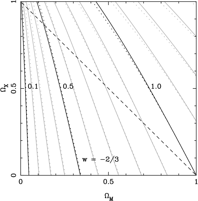
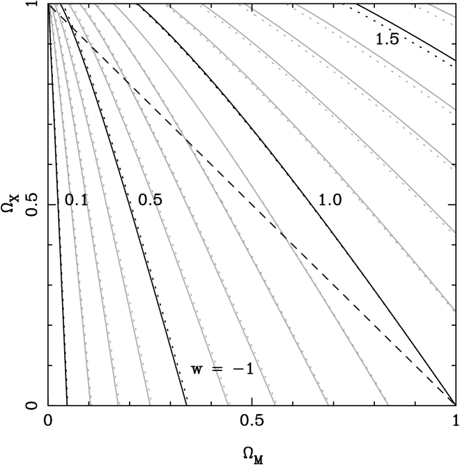
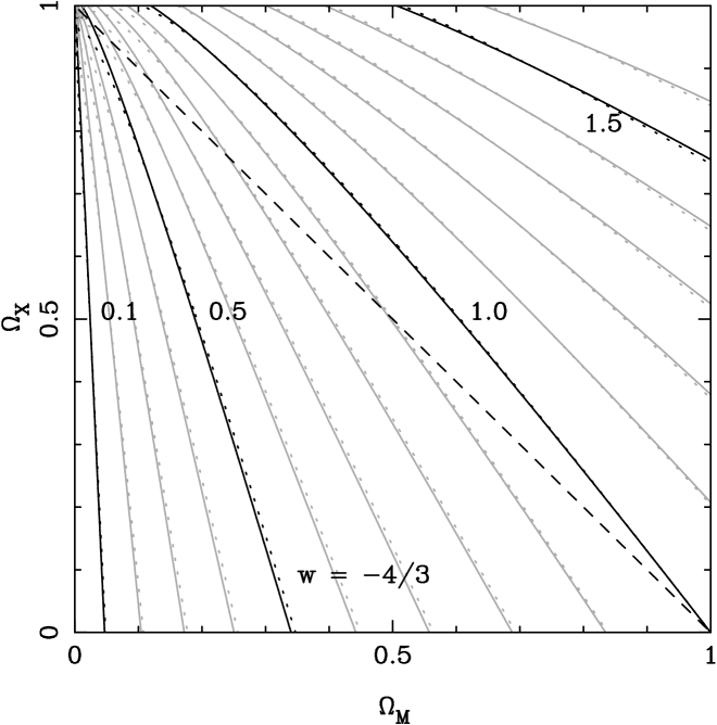
Figure 2: Plots showing contours of constant linear growth factor to present day for a selection of cosmologies (grey and black lines). The growth factor is normalised to unity for $\Omega_{M}=1$, $\Omega_{X}=0$. Increasing $w$ from $-4/3$ to $-2/3$, decreases the growth factor leading to behaviour more like that of an open Universe. Dotted contours are for the fitting formula of Eq. 20, together with Eqns. 19 & 21. The dashed line highlights flat cosmological models.

Eq. 14 can easily be solved by numerical integration, and we show contours of different linear growth factor to present day in ($\Omega_{M}$,$\Omega_{X}$) space in Fig. 2 for constant $w=-2/3,-1,-4/3$. The linear growth factor is strongly dependent on $w$, with $w>-1$ models behaving more like open Universes than $w<-1$ models as the effect of the dark energy diminishes. For the linear growth factor in a variety of cosmological models with time dependent $w(a)$ see, for example, Doran, Schwindt & Wetterich (2001); Linder & Jenkins (2003).

For $\Lambda$ cosmologies, the growing mode solution to this equation is (Heath 1977)

$$D(a)=\frac{5\Omega_{M}}{2}E(a)\int^{a}_{0}\frac{da^{\prime}}{[a^{\prime}E(a^{\prime})]^{3}},$$ (15)

where $E(a)$ is given by Eq. 3. Although this integral can be easily solved numerically, it is common to use the approximation of Carroll, Press & Turner (1992), which follows from work in Lightman & Schechter (1990) and Lahav et al. (1991)

$$D(a)\simeq\frac{5\Omega_{M}(a)a}{2}\left[\Omega_{M}(a)^{4/7}-\Omega_{\Lambda}(a)\right.$$ (16)

$$\hskip 56.9055pt\left.+\left(1+\frac{\Omega_{M}(a)}{2}\right)\left(1+\frac{\Omega_{\Lambda}(a)}{70}\right)\right]^{-1}.$$

A general solution for the growing mode solution in dark energy cosmologies, equivalent to Eq. 15, has yet to be found. However, for flat cosmological models, with constant $w$, the solution can be written in terms of the hypergeometric function ${}_{2}F_{1}$ (Silveira & Waga 1994)

$$D(a)=a\,_{2}F_{1}\left[-\frac{1}{3w},\frac{w-1}{2w},1-\frac{5}{6w},-a^{-3w}\frac{1-\Omega_{M}}{\Omega_{M}}\right].$$ (17)

Writing the growth index as

$$\frac{d\ln\delta}{d\ln a}=\Omega_{M}^{\alpha}(a),$$ (18)

Wang & Steinhardt (1998) use Eq. 14 for the special case of flat cosmologies to give

$$\alpha\simeq\frac{3}{5-w/(1-w)}$$

$$\hskip 14.22636pt+\frac{3}{125}\frac{(1-w)(1-3w/2)}{(1-6w/5)^{3}}\left[1-\Omega_{M}(a)\right].$$ (19)

This led Basilakos (2003) to extend the approximation of Carroll, Press & Turner (1992) given by Eq. 16 to the case of $w\neq-1$

$$D(a)\simeq\frac{5\Omega_{M}(a)a}{2}\left[\Omega_{M}(a)^{\alpha}-\Omega_{X}(a)\right.$$ (20)

$$\hskip 56.9055pt\left.+\left(1+\frac{\Omega_{M}(a)}{2}\right)\left(1+\mathcal{A}\Omega_{X}(a)\right)\right]^{-1},$$

with $\alpha$ given by Eq. 19, and $\mathcal{A}\simeq 1.742+3.343w+1.615w^{2}$. In Fig. 3 we plot the $\mathcal{A}$ values required to match Eq. 20 to the true linear growth factor (given by Eq. 17), for flat cosmological models with $0.1<\Omega_{M}<0.9$ as a function of $w$ (grey lines). The fit of Basilakos (2003) is shown by the dashed line. This is a poor fit for $w<-1$, so instead, we propose

$$\mathcal{A}=\frac{-0.28}{w+0.08}-0.3,$$ (21)

shown by the black line in Fig. 3.

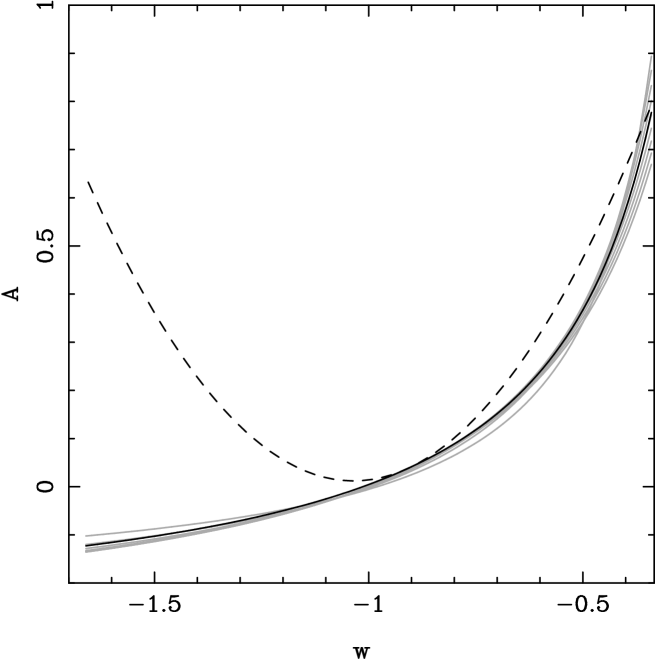
Figure 3: Plot showing the true value of $\mathcal{A}$ in Eq. 20 as a function of $w$ for 9 flat cosmologies with $\Omega_{M}$ evenly spread between $0.1$ and $0.9$ (grey lines). For comparison we plot the fitting formula of Basilakos (2003) (dashed line) and for Eq. 21 (black line).

Eq. 21 has been determined by fitting to flat cosmological models with $0.1<\Omega_{M}<0.9$. For non-flat models, the approximation of Eq. 20 remains a good fit. In Fig. 2, the dotted contours are for the fitting formula of Eq. 20, together with Eqns. 19 & 21, compared with the true value of $D_{0}$ given by the solid contours. The fitting formula fails for $\Omega_{M}<<0.1$, but for $\Omega_{M}>0.1$, the maximum error (with $0<\Omega_{X}<1$) is 3.8% for $w=-4/3$, 2.6% for $w=-1$ and 5.1% for $w=-2/3$. For comparison, the fitting formula of Carroll, Press & Turner (1992) given by Eq. 16 is accurate to 2.1% for $w=-1$ over this range of $\Omega_{M}$.

4 the critical density for collapse of spherical perturbations

We now calculate the critical overdensity for collapse of homogeneous spherical perturbations at present day in a homogeneous dark energy background. The method adopted is a development of that in Percival et al. (2000), where the critical overdensity in $\Lambda$ cosmologies was calculated. Solution schemes for an Einstein-de Sitter cosmology (Gunn & Gott 1972), for open cosmologies Lacey & Cole (1993) and for flat $\Lambda$ cosmologies (Eke, Cole & Frenk 1996) were summarised in Kitayama & Suto (1996). See also the solution scheme for $\Lambda$ cosmologies used by Barrow & Stein-Schabes (1984); Barrow & Saich (1993).

As in Section  3, we consider two spheres containing equal amounts of material: one of background material with radius $a$, and one of radius $a_{p}$ with a homogeneous change in overdensity. If the dark energy component is negligible, as at early times for $lim_{a\to 0}w(a)<-1/3$,

$$\left(\frac{da}{d(H_{0}t)}\right)^{2}=\frac{\Omega_{M}}{a}+\epsilon,$$ (22)

where $\epsilon$ is allowed to take any real value. For the background, $\epsilon=\Omega_{K}\equiv(1-\Omega_{M}-\Omega_{X})$ is the standard curvature constant. The matter density $\Omega_{M}$ is the same for both the perturbation and the background as the two spherical regions contain the same mass. Following Percival et al. (2000), a series solution for $a(H_{0}t)$ in the limit $H_{0}t\to 0$ can be obtained given by $a=\alpha(H_{0}t)^{2/3}+\beta(H_{0}t)^{4/3}+O[(H_{0}t)^{6/3}]$, where

$$\alpha=\left(\frac{9\Omega_{M}}{4}\right)^{1/3},\,\,\,\beta=\frac{3\epsilon}{20}\left(\frac{12}{\Omega_{M}}\right)^{1/3}.$$ (23)

Using the fact that the spheres contain equal mass,

$$\lim_{H_{0}t\to 0}\delta(H_{0}t)=\frac{3}{\alpha}(\beta-\beta_{p})(H_{0}t)^{2/3}+O[(H_{0}t)^{4/3}].$$ (24)

Substituting Eq. 23 into Eq. 24 gives that

$$\lim_{H_{0}t\to 0}\delta(H_{0}t)=$$

$$\hskip 28.45274pt\frac{3}{5}\left(\frac{3}{2\Omega_{M}}\right)^{2/3}\left[(1-\Omega_{M}-\Omega_{X})-\epsilon_{p}\right](H_{0}t)^{2/3}.$$ (25)

We now extrapolate this limiting behaviour to present day, using the linear growth factor to extrapolate the normalisation of the density field from early times. This gives

$$\delta_{c}=D_{0}\lim_{H_{0}t\to 0}\left[\frac{\delta(t)}{D(t)}\right],$$ (26)

where $D_{0}$ is the linear growth factor to present day. Given the normalisation of $D(t)$ adopted in Section 3, $\lim_{H_{0}t\to 0}D(H_{0}t)=\alpha(H_{0}t)^{2/3}$, where $\alpha$ is given by Eq. 23. We can therefore write $\delta_{c}$ as

$$\frac{\delta_{c}}{D_{0}}=\frac{3}{5\Omega_{M}}\left[(1-\Omega_{M}-\Omega_{X})-\epsilon_{p}\right].$$ (27)

This formula relates the linearly extrapolated overdensity $\delta_{c}$ to the initial curvature of the perturbation for cosmological models in which the dark energy becomes negligible as $H_{0}t\to 0$.

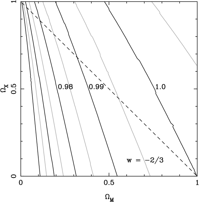
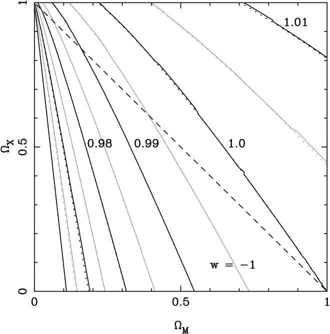
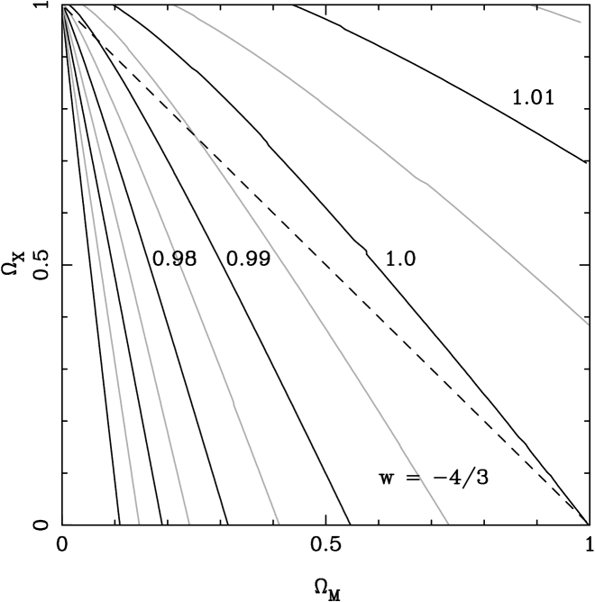
Figure 4: Plots showing contours of constant critical overdensity for a selection of cosmologies (grey and black lines) with constant $w$. Contours are plotted as a ratio of $\delta_{\rm EdS}$ as given by Eq. 29 from $0.96\delta_{\rm EdS}$ to $1.02\delta_{\rm EdS}$ at intervals of $0.005\delta_{\rm EdS}$. For the $w=-1$ cosmology we also plot the values determined by accurately solving Eq. 28 using standard Elliptical integrals (dotted lines). The difference between solid and dotted lines are caused by the numerical integration of Eqns 30, 31 & 32. The dashed line highlights flat cosmological models (as in Fig. 2).

4.1 case 1: cosmological constant

For $\Lambda$ cosmologies, the curvature of the perturbation (and energy) is conserved through the Friedmann equation

$$\left(\frac{da_{p}}{d(H_{0}t)}\right)^{2}=\frac{\Omega_{M}}{a_{p}}+\epsilon_{p}+\Omega_{\Lambda}a_{p}^{2}.$$ (28)

This equation defines a mini-cosmology, so using the methodology of Section 2, the requirement for collapse can be seen to be $-\epsilon_{p}^{3}>27\Omega_{\Lambda}\Omega_{M}^{2}/4$ (compare with Eq. 8). Given a perturbation that collapses, the time taken can be found by integrating Eq. 28, which can be reduced to a function of standard Elliptical integrals.

If $\Omega_{\Lambda}=0$, Eq. 28 can be solved analytically and, for an Einstein-de Sitter cosmology, the critical overdensity for collapse at present day reduces to

$$\delta_{\rm EdS}\equiv\frac{3}{20}(12\pi)^{2/3}\simeq 1.686,$$ (29)

which was first derived by Gunn & Gott (1972).

4.2 case 2: general $w(a)$ cosmologies

When the dark energy does not cluster, the energy within a spherical perturbation is not conserved (a comprehensive discussion of this is given in Weinberg & Kamionkowski 2003). Although this means that we cannot use Eq. 28 to determine the behaviour of the perturbation, we can still use the cosmology equation (Eq. 11). Wang & Steinhardt (1998) provide a boundary value problem for solving this second order differential equation, setting the boundary at the turn-around time. However, given the relatively straightforward initial evolution considered above, it is far simpler to set up an initial value problem (in either $a_{p}$ or $\delta$) to determine the subsequent behaviour. In a recent paper, Chiba, Takahashi & Sugiyama (2005) have also determined the limiting initial conditions for the differential equations, working directly from the cosmology equation. However, it is perhaps more intuitive to link the critical overdensity to the initial curvature of the perturbation (Eq. 27).

To see how this proceeds from the derivation above, suppose that we know $\delta_{c}$. Then Eq. 27 can be used to find the initial curvature $\epsilon_{p}$. The initial conditions, $a_{p}$, $\delta$, and $da_{p}/dt$ at some small, but finite $a$ can be obtained by substituting $\epsilon_{p}$ into Eqns 22 & 25.

Given these initial conditions, the evolution of the perturbation is uniquely specified by three equations: the cosmology equation for the perturbation and the background, and the Friedmann equation for the background. For completeness we repeat these equations here.

$$\frac{1}{a_{p}}\frac{d^{2}a_{p}}{d(H_{0}t)^{2}}=-\frac{1}{2}\left[\Omega_{M}a_{p}^{-3}+(3w(a)+1)\Omega_{X}a^{f(a)}\right],$$ (30)

$$\frac{1}{a}\frac{d^{2}a}{d(H_{0}t)^{2}}=-\frac{1}{2}\left[\Omega_{M}a^{-3}+(3w(a)+1)\Omega_{X}a^{f(a)}\right],$$ (31)

$$\frac{1}{a^{2}}\left[\frac{da}{d(H_{0}t)}\right]^{2}=\Omega_{M}a^{-3}+\Omega_{K}a^{-2}+\Omega_{X}a^{f(a)}.$$ (32)

By setting the initial value for the solution of these equations, we avoid any issues to do with symmetry: for general $w(a)$ cosmologies, not only is Eq. 28 invalid, but additionally the evolution of $a_{p}$ in time is no longer symmetric about the point of maximum expansion, because the effect of the dark energy is not symmetric about this point. This asymmetry is automatically accounted for by solving these equations from an initial value. In fact, this asymmetry leads to potentially interesting behaviour for the spherical perturbations: given the right initial conditions, perturbations can start to recollapse (turn-around), but then the repulsive force of the dark energy can cause re-expansion (Chiba, Takahashi & Sugiyama 2005).

In Fig. 4, we show contours of constant $\delta_{c}$ as a function of $\Omega_{M}$ and $\Omega_{X}$ for constant $w=-4/3,-1,-2/3$. Contours are plotted as a function of $\delta_{\rm EdS}$ as given by Eq. 29. As $\Omega_{X}\to 0$, the solutions asymptote towards the open Universe values calculated by Lacey & Cole (1993). For $\Omega_{X}>0$, we see that decreasing $w$ from $-2/3$ to $-4/3$ increases the effect of the dark energy. As for the linear growth factor, $w>-1$ cosmologies behave more like open cosmologies than those with $w<-1$: decreasing $w$ increases the importance of the dark energy for calculating $\delta_{c}$. The critical overdensities for collapse in a variety of cosmologies with varying $w(a)$ are compared in Mota & van de Bruck (2004).

5 the evolution of the critical overdensity

The evolution of the critical overdensity for collapse $\delta_{c}(a)$, is usually defined as follows: for a cosmological model with parameters $\Omega_{M}$ & $\Omega_{X}$, $\delta_{c}(a)$ gives the overdensity for a perturbation that collapses at scale factor $a$, normalised at present day. For example if we had a density field (and associated power spectrum) normalised at present day, then $\delta_{c}(a)$ (where $a$ does not necessarily equal 1) relates to spherical perturbations in this density field that collapse at scale factor $a$. $\delta_{c}$ is the particular case for perturbations that collapse at present day: perturbations that collapse earlier obviously have to be significantly more overdense. To calculate $\delta_{c}(a)$, when integrating the Friedmann equation (Eq. 28) for $\Lambda$ cosmologies, or numerically integrating Eqns. 30, 31 & 32 we would look for collapse at scale factor $a$ rather than $a=1$.

The rather weak evolution of the critical overdensity as a function of cosmological model (Fig. 4), means that the linear growth factor can be used to approximate $\delta_{c}(a)$: If $\delta_{c}$ is constant along a particular cosmological track then the evolution of $\delta_{c}(a)$ is purely driven by $D(a)^{-1}$. The only change in $\delta_{c}(a)$ between two collapse times is caused by the change in overall normalisation of the field, which can be seen by considering Eq. 26 for two cosmologies along a single cosmological track. The most obvious choice for the normalisation is $\delta_{\rm EdS}$, so the approximation will be correct in the limit as $a\to 0$,

$$\delta_{c}(a)\simeq\frac{D_{0}}{D(a)}\delta_{\rm EdS}.$$ (33)

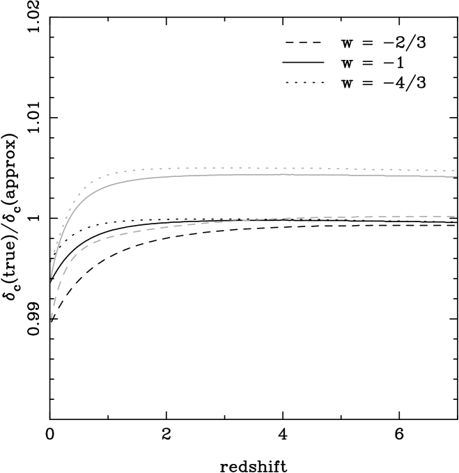
Figure 5: Plot showing the ratio between the critical overdensity for collapse $\delta_{c}(a)$ and the approximation given by Eq. 33, as a function of redshift for three different cosmological models (black lines). $\Omega_{M}=0.3$ and $\Omega_{X}=0.7$ are assumed, while $w$ is assumed to be constant with $w=-2/3,-1$, or $-4/3$. The grey lines shows the ratio between the true critical overdensity for collapse and the approximation, where the linear growth factor has itself been approximated by Eq. 20. The error in using the Einstein-de Sitter critical overdensity is of the same order as the error in the approximation of using the fitting formula of Eq. 20.

In order to demonstrate this approximation, in Fig. 5, we plot the ratio between the true critical overdensity $\delta_{c}(a)$ to the approximation given by Eq. 33 for three cosmological models with $\Omega_{M}=0.3$, $\Omega_{X}=0.7$, but with constant $w=-2/3,-1,-4/3$. As $a\to 0$, the approximation becomes more accurate. At $a=1$ (redshift $0$), the ratio is the same as the value of the surface contoured in Fig. 4. We also plot the approximate value of $\delta_{c}(a)$ calculated from Eq. 33, but with $D(a)$ and $D_{0}$ calculated using the approximation given by Eq. 20, Eq. 21 & Eq. 19 (grey lines). The error from using the approximation of Eq. 33 is of the same order as that from assuming the approximation to the linear growth factor for these cosmologies.

6 the mass function

The usefulness of the spherical model was emphasised when Press & Schechter considered smoothing the initial density field to determine the relative abundances of perturbations on different scales (Press & Schechter 1974: PS). When combined with the critical overdensity for collapse this provided a statistical model for the formation of structure in the Universe: smoothing the fluctuations leads to the masses of collapsed objects, while the spherical perturbation model gives the epoch of collapse for those perturbations that are sufficiently dense. Obviously such a simple model will fail in detail, particularly given the known complexities of asymmetrical gravitational collapse, and numerical simulations have now quantified these problems (Sheth & Tormen 1999; Jenkins et al. 2001). However PS theory has been incredibly successful and arguably still provides key insight into the processes at work in structure formation.

Two alternative formalisms are often considered for the collapse of perturbations in PS theory

1. The overdensity field is assumed to grow with the linear growth factor, and when perturbations reach the critical overdensity they are said to have collapsed.

2. Each overdense region is considered to be spherical and its collapse time is calculated as in Section 4.1.

Given the discussion in Section 5, it is easy to see that the first formalism, corresponding to a growing field, matches the approximation to $\delta_{c}(a)$ using the linear growth factor given by Eq. 33. The second formalism, which is adopted in the following analysis, corresponds to using the correct $\delta_{c}(a)$ for the spherical model.

Ma et al. (1999) considered the effect of quintessence on the mass transfer function. They provided fitting formulae for the ratio between the quintessence and $\Lambda$ cosmologies. However, if the dark energy only clusters on very large scales, the transfer function is only altered on these scales. If the power spectrum is normalised to $\sigma_{8}$ (the rms density fluctuation on scales of $8\,h\,{\rm Mpc}^{-1}$), then the scales usually of interest are not affected (Lokas, Bode & Hoffman 2004).

Figure 6: Plot showing the predicted mass function calculated using the fitting formula of Sheth & Tormen (1999) calculated for $\Omega_{M}=0.3$, $\Omega_{X}=0.7$ for three different values of $w$, and at three epochs corresponding to $a=1/3,1/2,1$. Because the power spectrum is normalised at present day, and $\delta_{c}$ is only weakly dependent on cosmology, then there is little difference between the predicted mass functions for $a=1$. As we go further back in time the difference becomes more severe because of the differing linear growth factors.

To demonstrate the effect of the dark energy equation of state on the mass function, we plot the cumulative mass function $N(>M)$, calculated using the numerical fit of Sheth & Tormen (1999) for 3 different cosmologies and 3 different epochs in Fig. 6. To determine the power spectrum we have used the fitting formulae of Eisenstein & Hu (1998) with $\Omega_{M}=0.3$, $\Omega_{b}/\Omega_{M}=0.15$, $\sigma_{8}=0.9$, $n_{s}=1$. The critical overdensity for collapse for $w=-2/3,-1$ & $-4/3$ and $\Omega_{X}=0.7$ was then calculated for $a=1/3,1/2,1$, corresponding to redshifts $z=2,1,0$. As expected, because the critical overdensity for collapse is only weakly dependent on cosmological parameters (Fig. 4), at $a=1$ (the epoch at which the power spectrum is normalised) we see very little difference in the predicted mass functions for different cosmologies. If the normalisation of the power spectrum had been constrained at a different epoch (for example by CMB fluctuations), then this would not be correct. The evolution of the mass function is strongly dependent on $w$ because of the effect on the evolution of $\delta_{c}(a)$ (Section 5) through the linear growth factor (Fig. 2). Consequently, determining the mass function at redshifts other than that used to normalise the power spectrum offers a stronger possibility of measuring $w(a)$. We will discuss the evolution of structure growth further in the next Section.

In order to compare with the observed cluster counts, we must convert from comoving position to observed angular position and redshift. The number of sources with mass $>M$ per unit solid angle in a redshift slice $dz$ is given by

$$N(>M,\Delta z)=\int_{z}^{z+\Delta z}\,dz\,N(>M)d_{\rm prop}^{2}\frac{dd_{\rm prop}}{dz},$$ (34)

where the proper distance $d_{\rm prop}$ is given by

$$d_{\rm prop}=\frac{c}{H_{0}}\int_{a}^{1}\,\frac{da}{a^{2}E(a)}.$$ (35)

This correction to the mass function reduces the significance of $w$ at low redshifts for masses of order $10^{14}{\rm\,M_{\odot}}$ (Solevi et al. 2005).

7 rate of structure growth

As discussed in the previous Section, the present day mass function does not provide a good test of $w$, although its evolution in time does. The Press-Schechter mass function (and the fitting formula of Sheth & Tormen 1999) is independent of epoch when written as a function of $\nu=\delta_{c}/\sigma_{M}$, where $\sigma_{M}$ is the rms fluctuation in the initial overdensity field on a scale corresponding to mass $M$. Consequently, it is easy to see that the evolution of the mass function is dependent on the rate at which $\delta_{c}$ changes, $d\delta_{c}(a)/da$. It is this quantity that we are testing by comparing mass functions at different epochs.

Extended Press-Schechter theory uses the smoothed initial overdensity field to create an analytic model for the build-up of structure (Bond et al. 1991; Bower 1991; Lacey & Cole 1993), in addition to providing a statistical model for the mass function. Within this extension to the theory, the rate at which structures grow is again driven by $d\delta_{c}(a)/da$ (Percival & Miller 1999; Percival et al. 2000; Cole et al. 2000; Miller, Percival & Croom 2005). Appendix A of Miller, Percival & Croom (2005) showed that the approximation of Eq. 33 can be easily extended to $d\delta_{c}(a)/da$ for $\Lambda$ cosmologies.

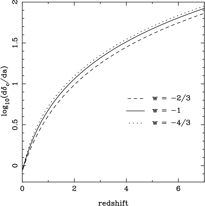
Figure 7: Plot showing the derivative of the critical overdensity for collapse with respect to the scale factor $d\delta_{c}(a)/da$ (black lines) and the approximation calculated from Eq. 33 (grey lines), as a function of redshift for three different cosmological models. $\Omega_{M}=0.3$ and $\Omega_{X}=0.7$ are assumed, while $w=-4/3,-1$, or $-2/3$. The approximation is so good that the grey lines are almost completely hidden behind the black lines.

Here, we extend this analysis to consider $d\delta_{c}(a)/da$ for $w\neq-1$ cosmologies. In Fig. 7 we show $d\delta_{c}(a)/da$ for three flat cosmological models with $\Omega_{M}=0.3$, and $w=-4/3,-1$, or $-2/3$ calculated using the derivation of Section 4.2 (black lines) and the fit of Eq. 33 (grey lines). In fact, the fit is so good that the grey lines are hardly visible in this plot. As expected $d\delta_{c}(a)/da$ is strongly dependent on the dark energy equation of state.

8 virialisation

The inhomogeneous nature of true perturbations means that they do not collapse to singularities, but instead stabilise at finite size. For $\Lambda$ cosmologies it is possible to use energy considerations to determine the final radius and density of the virialised perturbation (Lahav et al. 1991). The extension of this analysis to more general dark energy cosmologies has been considered by a number of authors (Wang & Steinhardt 1998; Horellou & Berge 2005; Maor & Lahav 2005).

Within a perturbation, the potential energy due to the matter $U_{G}$ and dark energy $U_{X}$ are given by (Horellou & Berge 2005; Maor & Lahav 2005)

$$U_{G}=-\frac{3GM^{2}}{5R},\,\,\,U_{X}=[1+3w(a)]\frac{4\pi GM}{10}\rho_{X}R^{2}.$$ (36)

These can be calculated from the Poisson Equation with pressure term. Note that there is some confusion in the literature about the exact form of $U_{X}$ and the $[1+3w(a)]$ term has sometimes been neglected in the past, although it is included in more recent work (Battye & Weller 2003; Horellou & Berge 2005). Even without this term, the discussion below about the lack of energy conservation within the perturbation remains valid, although the numerical results will obviously change.

For dark energy cosmologies the virial theorem, that a system with potential energy $U\propto R^{p}$ virialises with temperature $T=pU/2$, holds and $T=-\frac{1}{2}U_{G}+U_{X}$ at the epoch of virialisation. Assuming conservation of total energy between turn-around at $a_{\rm ta}$ and virialisation $a_{\rm vir}$ gives

$$U_{G}(a_{\rm ta})+U_{X}(a_{\rm ta})=\frac{1}{2}U_{G}(a_{\rm vir})+2U_{X}(a_{\rm vir}).$$ (37)

Substituting the definitions given by Eq. 36 leads to (Wang & Steinhardt 1998; Horellou & Berge 2005; Maor & Lahav 2005)

$$\left(1-[1+3w(a_{\rm ta})]\frac{q}{2}\right)x+[1+3w(a_{\rm vir})]\frac{qx^{3}}{y}=\frac{1}{2},$$ (38)

where

$$x = \frac{R_{\rm vir}}{R_{\rm ta}},$$

$$q = \frac{\Omega_{X}(a_{\rm ta})}{[1+\delta(a_{\rm ta})]\Omega_{M}(a_{\rm ta})},$$

$$y = \frac{\rho_{X}(a_{\rm ta})}{\rho_{X}(a_{\rm vir})}=\frac{a_{\rm ta}^{\,\,f(a_{\rm ta})}}{a_{\rm vir}^{\,\,f(a_{\rm vir})}}.$$ (39)

Here $q$ gives the ratio of the dark energy density to the matter density in the perturbation at turn-around. For $w=-1$, $y=1$ and Eq. 38 reduces to the formula of Lahav et al. (1991). For $w=-1/3$ or $\Omega_{X}=0$, we find $x=1/2$.

The above derivation was based on the assumption that total energy is conserved for the perturbation between turn-around and virialisation. This is a common assumption in the literature for cosmologies in which the dark energy remains homogeneous on the scales of the perturbations (e.g. Wang & Steinhardt 1998; Weinberg & Kamionkowski 2003; Battye & Weller 2003; Horellou & Berge 2005). Even in work that considers possible dark energy clustering, energy conservation has previously been assumed in the homogeneous case (see the discussion leading to equation 26 of Maor & Lahav 2005). However, the potential energy of the matter due to the presence of the dark energy $U_{X}$ ($U_{12}$ in the notation of Maor & Lahav 2005) is dependent on the dark energy density in the perturbation $\rho_{X}(a)$. The evolution of this density lies with the background, rather than the perturbation, so the total energy is not expected to be conserved: this is why we could not write down a Friedmann equation for the perturbation in Section 4. Obviously, if the total energy of the perturbation between turn-around and virialisation is not conserved, then Equation 37 does not hold.

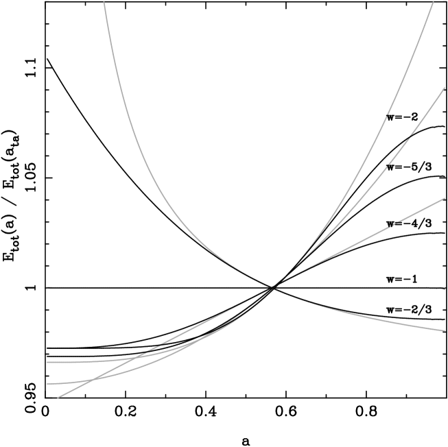
Figure 8: The total energy in an ideal homogeneous spherical perturbation (as modelled in Section 4), undergoing collapse to a singularity at $a=1$, relative to the energy at turn-around (black lines). $\Omega_{M}=0.3$ and $\Omega_{X}=0.7$ are assumed, with constant $w$ at the values shown. For general $w$, the total energy is not conserved. If the perturbations had remained at the turn-around size throughout their evolution, then the total energies would have evolved along the grey lines. The actual evolution in total energy lies between the line of constant total energy and the line of constant size for each cosmology.

In fact, we can consider two extreme situations. In the first, as above, the total energy at $a_{\rm vir}$ is the same as at $a_{\rm ta}$. In the second, we assume that the perturbation did not change size between the two epochs. Following the second assumption, the total energy in the system at $a_{\rm vir}$ would have been altered from that at $a_{\rm ta}$ by the change in the dark energy potential $U_{X,1}-U_{X,2}$, where

$$U_{X,1} = [1+3w(a_{\rm ta})]\frac{4\pi GM}{10}\rho_{X}(a_{\rm ta})R_{\rm ta}^{2},$$ (40)

$$U_{X,2} = [1+3w(a_{\rm vir})]\frac{4\pi GM}{10}\rho_{X}(a_{\rm vir})R_{\rm ta}^{2}.$$ (41)

We call using the dark energy potential $U_{X,1}$ to calculate the total energy in the perturbation at virialisation “fixing the energy at turn-around”, and using $U_{X,2}$ “fixing the energy at virialisation”. This is demonstrated in Fig. 8, where we plot the total energy in an ideal homogeneous perturbation undergoing collapse to a singularity at $a=1$ relative to the energy at turn-around (black lines), for a number of cosmologies. The total energy was calculated by combining the analysis of Section 4 with the definitions of potential energy of Eq. 36. Obviously if the total energy were constant we would find a horizontal line, as is the case when $w=-1$. If the perturbation did not evolve in size, with the radius fixed at the turn-around value, then the evolution of the total energy is shown by the grey lines. The actual total energy within the perturbation lies between these two extreme cases for each value of $w$ assumed.

For a more realistic perturbation that underwent virialisation rather than collapsing to a singularity, provided that the dark energy potential varies monotonically between $a_{\rm ta}$ and $a_{\rm vir}$, then the change in total energy in the system between turn-around and virialisation should still lie between these two cases: some of the change in total energy due to the dark energy remaining homogeneous will be converted into kinetic energy, and some will be “lost” to the background.

The second scenario, using $U_{X,2}$ to “fix” the energy at virialisation alters Eq. 38 to give

$$\left(1-[1+3w(a_{\rm vir})]\frac{q}{2y}\right)x+[1+3w(a_{\rm vir})]\frac{qx^{3}}{y}=\frac{1}{2},$$ (42)

with $x$, $y$, & $q$ defined as before. For $w=-1$ this equation again reduces to the formula of Lahav et al. (1991).

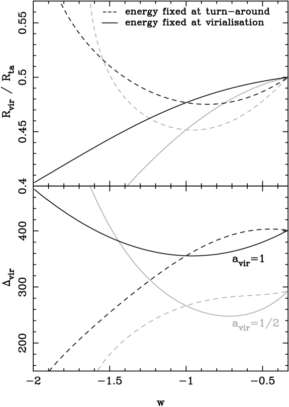
Figure 9: Upper panel: the ratio between the virialisation radius and maximum turn-around radius for a spherical perturbation that virialises at $a=1$ (black lines) or $a=1/2$ (grey lines), assumed to be the same as the epoch predicted for collapse of a homogeneous perturbation. We assume that $\Omega_{M}=0.3$, $\Omega_{X}=0.7$, and plot results as a function of constant $w$. The dashed and solid lines show two different calculations assuming conservation of energy based on the dark energy density either at turn-around, or at virialisation. Lower panel: as upper panel, but now showing the overdensity of the virialised system.

In the upper panel of Fig. 9 we plot $R_{\rm vir}/R_{\rm ta}$ in these two cases in a cosmology with $\Omega_{M}=0.3$, $\Omega_{X}=0.7$, as a function of constant $w$. We assume that virialisation occurs at the collapse epoch, set to be either the present day or $a=1/2$, for the homogeneous spherical model. For constant $w=-1/3$ we find $R_{\rm vir}/R_{\rm ta}=1/2$ as expected. For constant $w=-1$, the two solutions converge to the result of Lahav et al. (1991). For $-1<w<-1/3$, the component of the energy of the perturbation in the form of dark energy changes from turn-around to virialisation, and both energy conservation arguments predict different values of $R_{\rm vir}/R_{\rm ta}$, although the trend with $w$ is the same for both. However, for $w<-1$, the solutions diverge. It is easy to see why: for $w<<-1$, the dark energy becomes increasingly important at late times in the evolution of the Universe. For a solution that collapses at present day (for example), turn-around must happen at an epoch where the dark energy has yet to be cosmologically important. It is only between turn-around and virialisation that the dark energy becomes important. Setting the energy to be constant based on the dark energy density at virialisation simply continues the trend from $-1/3>w>-1$, with $\rho_{X}$ increasing as $w$ decreases, leading to a decrease in the potential due to the dark energy $U_{X}$, and a smaller $R_{\rm vir}/R_{\rm ta}$ ratio. However, setting the dark energy density at turn-around has the opposite effect: $\rho_{X}$ decreases, leading to $U_{X}$ and $R_{\rm vir}/R_{\rm ta}$ increasing. For perturbations that turn-around, but do not collapse, the dark energy density increases so rapidly between turn-around and virialisation that the predicted $R_{\rm vir}/R_{\rm ta}$ keeps increasing (although virialisation is never reached because the perturbation can never stabilise).

In the lower panel of Fig. 9 we plot the overdensity at virialisation $\Delta_{\rm vir}$, calculated for the two values of the total energy. As can be seen, the result has a very similar dependence on $w$ as described above for $R_{\rm vir}/R_{\rm ta}$. It is clear that further analysis is required before measurements that depend on $\Delta_{\rm vir}$ can be used to constrain $w$. The answer may lie in numerical simulations of the time evolution of the perturbation leading to virialisation, possibly of the form of Engineer, Kanekar & Padmanabhan (2000), or possibly standard N-body simulations (Meneghetti et al. 2005; Bartelmann et al. 2005). Such simulations will need to consider the evolution of total energy with time as well as the changing epoch of virialisation: given the possible strong effect of the dark energy, it seems clear that the assumption that virialisation of the perturbation occurs at the collapse time predicted in the homogeneous case will also break down in addition to the conservation of total energy.

9 conclusions

The presence of dark energy alters the way in which cosmological structures grow, thus providing an observational signature that is complementary to geometrical effects. The structure growth is dependent on the normalisation of the dark energy density $\Omega_{X}$, its equation of state, and sound speed, which determines how this component clusters. In this paper we have only considered the effect of the first two of these properties, assuming that the dark energy remains homogeneous on the scales of interest due to a high sound speed. The spherical top-hat model has been used to determine the linear growth rate and non-linear collapse overdensity threshold. The equations provided have allowed for general $w(a)$. We have also considered the statistics of observed structures through the mass function and its evolution. Finally, the virialisation of perturbations has been considered and a new argument has been presented demonstrating the importance of the lack of energy conservation within a perturbation. It is clear that more work is required before observations that use arguments based on the energy in perturbations can be used to constrain the dark energy. However, there is clearly tremendous potential for future observations to detect the cosmological effects of dark energy in sufficient detail to pin down its properties. Proving that $w\neq-1$, or indeed that $w=-1$ would be an exciting result, and remains one of the goals of modern cosmology.

References

- Barrow & Stein-Schabes (1984) Barrow J.D., Stein-schabes J., 1984, Phys. Lett. A, 103, 315
- Barrow & Saich (1993) Barrow J.D., Saich P., 1993, MNRAS, 262, 717
- Bartelmann et al. (2005) Bartelmann M., Dolag K., Perrotta F., Baccigalupi C., Moscardini L., Meneghetti M., Tormen G., 2005, NewAR, 49, 199
- Basilakos (2003) Basilakos S., 2003, ApJ, 590, 636
- Bassett, Corasaniti & Kunz (2004) Bassett B.A., Corasaniti P.S., Kunz N., 2004, ApJ, 617, L1
- Battye & Weller (2003) Battye R.A., Weller J., 2003, Phys. Rev. D, 68, 083506
- Birkhoff (1923) Birkhoff G., 1923, Relativity and Modern Physics, Harvard University Press, Cambridge, Mass.
- Bond et al. (1991) Bond J.R., Cole S., Efstathiou G., Kaiser N., 1991, ApJ, 379, 440
- Bower (1991) Bower R.G., 1991, MNRAS, 248, 332
- Caldwell, Dave & Steinhardt (1998a) Caldwell R.R., Dave R., Steinhardt P.J., 1998a, Astrophysics & Space sciences, 261, 303
- Caldwell, Dave & Steinhardt (1998b) Caldwell R.R., Dave R., Steinhardt P.J., 1998b, Phys. Rev. Let., 80, 8
- Caldwell, Kamionkowski & Weinberg (2003) Caldwell R.R., Kamionkowski M., Weinberg N.N., 2003, Phys. Rev. Let., 91, 071301
- Carroll, Press & Turner (1992) Carroll S.M., Press W.H., Turner E.L., 1992, ARA&A, 30, 499
- Chiba, Takahashi & Sugiyama (2005) Chiba T., Takahashi R., Sugiyama N., 2005, astro-ph/0501661
- Cole et al. (2000) Cole S., Lacey C.G., Baugh C.M., Frenk C.S., 2000, MNRAS, 319, 168
- Cole et al. (2005) Cole S., et al., 2005, MNRAS submitted, astro-ph/0501174
- Dave, Caldwell & Steinhardt (2002) Dave R., Caldwell R.R., Steinhardt P.J., 2002, astro-ph/0206372
- de Araujo (2005) de Araujo J.-C. N., 2005, astro-ph/0503099
- de Bernardis et al. (2000) de Bernardis, et al., 2000, Nature, 404, 955
- Doran, Schwindt & Wetterich (2001) Doran M., Schwindt J.-M., Wetterich C., 2001, Phy. Rev. D, 64, 123520
- Efstathiou et al. (2002) Efstathiou G., et al., 2002, MNRAS, 330, 29
- Eisenstein & Hu (1998) Eisenstein D.J., Hu W., 1998, ApJ, 496, 605
- Eke, Cole & Frenk (1996) Eke V.R., Cole S., Frenk C.S., 1996, MNRAS, 282, 263
- Engineer, Kanekar & Padmanabhan (2000) Engineer S., Kanekar N., Padmanabhan T., 2000, MNRAS, 314, 279
- Felten & Isaacman (1986) Felten J.E., Isaacman R., 1986, Rev. Mod. Phys., 58, 689
- Glanfield (1966) Glanfield J.R., 1966, MNRAS, 131, 271
- Gunn & Gott (1972) Gunn J.E., Gott J.R., 1972, ApJ, 176, 1
- Halverson et al. (2002) Halverson N.W., et al., 2002, ApJ, 568, 38
- Hannestad (2005) Hannestad S., 2005, astro-ph/0504017
- Heath (1977) Heath D.J., 1977, MNRAS, 179, 351
- Hinshaw et al. (2003) Hinshaw G., et al., 2003, ApJS, 148, 135
- Horellou & Berge (2005) Horellou C., Berge J., 2005, MNRAS submitted, astro-ph/0504465
- Hu & Scranton (2004) Hu W., Scranton R., 2004, Phys. Rev. D, 70, 063530
- Jassal, Bagla & Padmanabhan (2004) Jassal H.K., Bagla J.S., Padmanabhan T., 2004, MNRAS, 356, L11
- Jenkins et al. (2001) Jenkins A., Frenk C.S., White S.D.M., Colberg J.M., Cole S., Evrard A.E., Couchman H.M.P., Yoshida N., 2001, MNRAS, 321, 372
- Johri (2004) Johri V.B., 2004, astro-ph/0409161
- Kitayama & Suto (1996) Kitayama T., Suto Y., 1996, ApJ, 469, 480
- Kujat et al. (2002) Kujat J., Linn A.M., Scherrer R.J., Weinberg D.H., 2002, ApJ, 572, 1
- Lacey & Cole (1993) Lacey C., Cole S., 1993, MNRAS, 262, 627
- Lahav et al. (1991) Lahav O., Lilje P.B., Primack J.R., Rees M.J., 1991, MNRAS, 251, 128
- Lee et al. (2001) Lee A.T., et al., 2001, ApJ, 561, L1
- Lightman & Schechter (1990) Lightman A.P., Schechter P.L., 1990, ApJS, 74, 831
- Linder & Jenkins (2003) Linder E.V., Jenkins A., 2003, MNRAS, 346, 573
- Lokas, Bode & Hoffman (2004) Lokas E.L., Bode P., Hoffman Y., 2004, MNRAS, 349, 595
- Ma et al. (1999) Ma C.-P., Caldwell R.R., Bode P., Wang L., 1999, ApJ, 521, L1
- Manera & Mota (2005) Manera M., Mota D.F., 2005, MNRAS submitted, astro-ph/0504519
- Maor et al. (2002) Maor I., Brustein R., McMahon J., Steinhardt P.J., 2002, Phys. Rev. D, 65, 123003
- Maor & Lahav (2005) Maor I., Lahav O., 2005, astro-ph/0505308
- Meneghetti et al. (2005) Meneghetti M., Bartelman M., Dolag, K., Perrotta F., Baccigalupi C., Moscardini L., Tormen G., 2005, NewAR, 49, 111
- Miller, Percival & Croom (2005) Miller L., Percival W.J., Croom S.M., 2005, MNRAS submitted, astro-ph/0506591
- Moles (1991) Moles M., 1991, ApJ, 382, 369
- Mota & van de Bruck (2004) Mota D.F., van de Bruck C., 2004, A&A, 421, 71
- Nunes & Mota (2004) Nunes N.J., Mota D.F., 2004, MNRAS submitted, astro-ph/0409481
- Pearson et al. (2003) Pearson T.J., et al., 2003, ApJ, 591, 540
- Peebles (1980) Peebles P.J.E., 1980, The Large Scale Structure of the Universe, Princeton University Press
- Peebles & Ratra (1988) Peebles P.J.E., Ratra B., 1988, ApJ, 325, 17
- Peebles & Ratra (2003) Peebles P.J.E., Ratra B., 2003, Rev. Mod. Phys., 75, 559
- Percival & Miller (1999) Percival W.J., Miller L., 1999, MNRAS, 309, 823
- Percival et al. (2000) Percival W.J., Miller L., Peacock J.A., 2000, MNRAS, 318, 273
- Percival et al. (2001) Percival W.J., et al., 2001, MNRAS, 327, 1297
- Percival et al. (2002) Percival W.J., et al., 2002, MNRAS, 337, 1068
- Perlmutter et al. (1999) Perlmutter S., et al., 1999, ApJ, 517, 565
- Press & Schechter (1974) Press W., Schechter P., 1974, ApJ, 187, 425
- Ratra & Peebles (1988) Ratra B., Peebles P.J.E., 1988, ApJ, 325, 17
- Riess et al. (1998) Riess A.G., et al., 1998, AJ, 116, 1009
- Scott et al. (2003) Scott P.F., et al., 2003, MNRAS, 341, 1076
- Sheth & Tormen (1999) Sheth R.K., Tormen G., 1999, MNRAS, 108, 119
- Silveira & Waga (1994) Silveira V., Waga I., 1994, Phys. Rev. D, 64, 4890
- Solevi et al. (2005) Solevi P., Mainini R., Bonometto S.A., Maccio A.V., Klypin A., Gottlober S., 2005, MNRAS submitted, astro-ph/0504124
- Spergel et al. (2003) Spergel D.N., 2003, ApJS, 148, 175
- Tegmark et al. (2004a) Tegmark M., et al., 2004a, ApJ, 606, 702
- Tegmark et al. (2004b) Tegmark M., et al., 2004b, Phys. Rev. D, 69, 103501
- Wang & Steinhardt (1998) Wang L., Steidhardt P.J., 1998, ApJ, 508, 483
- Wang et al. (2000) Wang L., Caldwell R.R., Ostriker J.P., Steidhardt P.J., 2000, ApJ, 530, 17
- Weinberg & Kamionkowski (2003) Weinberg N.N., Kamionkowski M., 2003, MNRAS, 341, 251
- Wetterich (1988) Wetterich C., 1988, Nucl. Phys. B, 302, 668
- Zel’dovich & Barenblatt (1958) Zel’dovich Ya.B., Barenblatt G., 1958, Sov. Phys. Dokl. 3, 44-47