The Time Delays of Gravitational Lens HE 0435–1223:
An Early-Type Galaxy With a Rising Rotation Curve

Abstract

We present Hubble Space Telescope images and 2 years of optical photometry of the quadruple quasar HE 0435–1223. The time delays between the intrinsic quasar variations are $\Delta t_{AD}=-14.37_{-0.85}^{+0.75}$, $\Delta t_{AB}=-8.00_{-0.82}^{+0.73}$, and $\Delta t_{AC}=-2.10_{-0.71}^{+0.78}$ days. We also observed non-intrinsic variations of $\sim$$0.1$ mag yr^-1 that we attribute to microlensing. Instead of the traditional approach of assuming a rotation curve for the lens galaxy and then deriving the Hubble constant ($H_{0}$), we assume $H_{0}=(72\pm 7)$ km s^-1 Mpc^-1 and derive constraints on the rotation curve. On the scale over which the lensed images occur ($1\farcs 2=5h^{-1}$ kpc $\simeq 1.5R_{e}$), the lens galaxy must have a rising rotation curve, and it cannot have a constant mass-to-light ratio. These results add to the evidence that the structures of early-type galaxies are heterogeneous.

1 Introduction

Variability of the multiple images of a gravitationally lensed quasar results from two distinct phenomena: intrinsic flux variations of the background quasar, and microlensing by stars or other compact masses in the foreground galaxy. Intrinsic variations are seen in different quasar images at different times, owing to the different optical path length and gravitational time delay associated with each image. Time delays have been measured in about 10 systems, with varying levels of accuracy and difficulty of interpretation, as recently reviewed by Kochanek & Schechter Kochanek04 (2004) and Kochanek Kochanek05 (2005). Microlensing, by contrast, is an extrinsic phenomenon, arising from the granularity of the lensing mass distribution. The granularity causes the image magnification to become a very complex function of the source position (a “caustic pattern”). As the source moves with respect to the pattern, uncorrelated variability is observed in the lensed images. Microlensing has been observed in many quasar light curves, most notably in the intensively monitored systems Q 2237+0305 and Q 0957+564 (see the recent review by Wambsganss 2005).

Observations of the intrinsic and extrinsic variations have traditionally been sought for entirely different reasons. Most the effort in measuring time delays has been motivated by the prospect of determining the Hubble constant ($H_{0}$) independently of local distance indicators (Refsdal 1964). Microlensing is traditionally seen as either noise in the cosmological measurement, or a means of studying the quasar emitting region and the microlens mass function. Given some recent developments in both observational cosmology and gravitational lensing theory, we find it useful to regard both time delays and microlensing variability as complementary probes of the structure and composition of galaxy halos over a particularly interesting range of galactocentric distances.

In the Cold Dark Matter (CDM) paradigm, galaxies have an inner region that is predominantly composed of baryons, and an outer region that is predominantly composed of dark matter particles. Most of the dark matter is smoothly distributed, but a modest fraction ($\sim$1%) exists in clumps, which are sometimes referred to as CDM “satellites” or “substructures” (e.g. Kauffmann Kauffmann93 (1993), Moore et al. Moore99 (1999), Klypin et al. Klypin99 (1999), Bode, Ostriker & Turok Bode01 (2001), Zentner & Bullock Zentner03 (2003)). For a massive early-type galaxy, the transition region between baryon dominance and dark-matter dominance is typically a few effective radii ($R_{e}$) from the center. Observations that are sensitive to the mass distribution in this transition region have resulted in confusing and apparently contradictory picture. There is much evidence suggesting that galaxies have nearly flat rotation curves (isothermal lens models) extending from the inner regions (see, e.g. Gerhard et al. 2001; Rusin & Kochanek 2003; Winn, Rusin, & Kochanek 2004, Treu & Koopmans 2004) but there are some interesting counter-examples (e.g. Romanowsky et al. Romanowsky03 (2003), Treu & Koopmans Treu2002p6 (2002)).

The typical Einstein radius of a gravitational lens galaxy also happens to be several effective radii, and hence the multiple images of a background quasar tend to occur within the baryon $\rightarrow$ dark-matter transition region. Lensing observations are thereby capable of providing constraints on the mass distribution in that region. Furthermore, while traditional dynamical observations are sensitive to the total enclosed mass within some radius, time delays and microlensing depend upon the local surface density and its degree of granularity, which are often of greater interest.

First, consider time delays. Kochanek (2002) showed that time delays depend upon a combination of $H_{0}$ and the surface mass density $\langle\kappa\rangle=\langle\Sigma\rangle/\Sigma_{c}$ near the images, with $\Delta t\propto(1-\langle\kappa\rangle)/H_{0}$ to lowest order. Kochanek (2003) analyzed the 4 systems that have a simple lens geometry and for which accurate time delays, astrometry and photometry were available: PG 1115+080, SBS 1520+530, CLASS B1600+434, and HE 2149-2745. He found that the lens galaxies in those systems have similar surface densities (with a scatter in $\kappa$ of less than 0.07), but together they present a problem for either CDM theory or the consensus value of $H_{0}$. If the Hubble constant is $H_{0}=(72\pm 7)$ km s^-1 Mpc^-1, as suggested by Cepheid-based measurements (Freedman et al. 2001) and analyses of microwave background fluctuations (Spergel et al. 2003), then all four lens galaxies must have surface densities $\langle\kappa\rangle\simeq 0.2$, which is close to what one would expect from a model with a constant mass-to-light ratio ($M/L$). Only if $H_{0}\simeq 50$ km s^-1 Mpc^-1 can they have $\langle\kappa\rangle\simeq 0.5$, as one would expect from a galaxy with a flat rotation curve. To make progress we should (1) improve upon the accuracies of many of the existing time delay measurements, some of which have uncertainties of 20% or worse; (2) measure delays in more systems, to see whether the result is a fluke (and, by extension, whether galaxies are heterogeneous); and (3) measure time delays in systems for which independent dynamical measurements are available; and (4) test for the effects and possible biases that are expected to be caused by variations in lens galaxy environments, by measuring delays for lenses in groups or clusters.

Next, consider microlensing. The character of the time variability in a microlensing light curve depends upon the local surface density at the position of the quasar image, and upon the fraction of that surface density that is composed of stars ($\kappa_{\star}/\kappa$). A statistical analysis of the instantaneous flux ratios of an ensemble of lenses has shown that there is a clear difference between the magnifications of images that are minima of the time-delay surface, and the magnifications of saddle-point images. This provides evidence that the stars represent no more than about 20% of the total surface density of the lens galaxies at the positions of the quasar images (Schechter & Wambsganss 2002, Kochanek & Dalal 2004). This, in turn, supports the standard isothermal models (which have considerable dark matter near the lensed images) and argues against constant-$M/L$ models. It should be possible to go beyond the ensemble analysis and analyze the light curves of individual systems in detail, now that there is a method for analyzing quasar microlensing light curves of arbitrary complexity (Kochanek 2004). This algorithm can be used to derive estimates of all the interesting physical variables, including $\kappa$, $\kappa_{*}$ and the mean stellar mass $\langle M\rangle$. Unfortunately, with the exception of Q 2237+030, the necessary data for such analyses is lacking.

With these motivations, we have undertaken a campaign to monitor a large number of gravitational lenses using a network of optical telescopes. Our aim is to obtain accurate multi-year light curves for approximately 25 systems, with a a time sampling of 1-2 points per week whenever a target is observable. We also rely on observations with the Hubble Space Telescope (HST ) to provide the accurate photometry and astrometry that are necessary for lens modeling. This paper, which examines the particular lens HE 0435–1223, is the first in what we hope will be a long series of new or improved time delay measurements, microlensing detections, and constraints on the structures of lens galaxies.

The quadruple-image quasar HE 0435–1223 was discovered by Wisotzki et al. (2002). The background quasar (“source”) has a redshift of $z_{s}=1.689$. The redshift of the lens galaxy was recently measured by Morgan et al. (2004) to be $z_{l}=0.4541$. Evidence of microlensing at optical wavelengths was presented previously by Wisotzki et al. (2003), based on integral-field spectrophotometry. In the following section, we present new HST  images as well as a re-analysis of previously presented images. In § 3 we discuss the design of our lens monitoring campaign and data-reduction pipeline, and present 2 years of photometry of HE 0435–1223. We introduce a new method for analyzing gravitational lens light curves, which is designed to separate the intrinsic variations from the microlensing variations, and to determine the time delays between all 4 quasar images. In § 4 we present a comprehensive study of the constraints on the mass distribution of the lens galaxy that are provided by the combination of time delay measurements and the HST  data. In the final section, we summarize our conclusions and draw a comparison with the results of other time-delay measurements.

Unless otherwise stated, we assume a flat cosmological model with $\Omega_{\rm M}=0.3$. Given the source and lens redshifts, the conversion from angular to physical scales is $1\farcs 0=4.05h^{-1}$ kpc (with $H_{0}=100h$ km s^-1 Mpc^-1), the critical surface density is $\Sigma_{c}=5.18\times 10^{10}$ $h^{-1}M_{\odot}/$arcsec², and the relation between velocity dispersion and Einstein radius $b$ for a singular isothermal sphere (SIS) is $\sigma=235\sqrt{b/1\farcs 0}$ km s^-1.

2 Hubble Space Telescope Observations

We have observed HE 0435–1223 in the V (F555W), I (F814W) and H (F160W) bands using HST. The 2000 s V-band and 1450 s I-band images were both obtained as five dithered sub-images with the Wide Field Channel (WFC) of the Advanced Camera for Surveys (ACS) on 2003 August 18. The ACS images were reduced using the Pyraf-based MULTIDRIZZLE package. The 2560 sec H-band image was obtained as four dithered sub-images on 2004 January 10 using the Near-Infrared Camera and Multi-Object Spectrograph (NICMOS). These data were reduced using our own NICRED software (see Lehár et al. 2000). Since the V and I band images have already been presented by Morgan et al. (2004), we focus here on the new H-band image, shown in Fig. 1. We have labeled the four quasar images A–D, the elliptical lens galaxy G, and a nearby (SBb) spiral galaxy G22, following the nomenclature of Morgan et al. (2004). The quasar host galaxy has been stretched into a nearly complete Einstein ring, which is prominent in the H-band image after the quasars and lens galaxy have been subtracted.

We fitted the H-band image with a photometric model consisting of point sources (representing the quasars), a de Vaucouleurs bulge (the lens galaxy), a de Vaucouleurs bulge and an exponential disk (the neighboring galaxy G22), and a lensed exponential disk for the host galaxy. All of these were convolved with a PSF model and then a least-squares fit to the image was performed, following the procedures of Lehár et al. (2000). The PSF model was selected from a series of 8 images of bright stars that were observed for this purpose (Yoo et al. 2005). We tried each of the 8 stars as a PSF model and for the final analysis we selected the star that resulted in the smallest residuals when applied to the HE 0435–1223 image. In our previous experience with subtracting quasar images with NICMOS, we have found that there are often significant residuals near the Airy ring of the diffraction pattern. For this reason, we included extra model parameters that allow for a distortion of the PSF model, which resulted in a modest improvement. After finding the best fit to the H-band image, we fitted the same model to the V and I-band images, holding the astrometric and structural parameters fixed and optimizing only the fluxes. In this manner we estimated the colors of all the objects. Table 2 presents the astrometric and photometric results from an analysis of the HST  images.

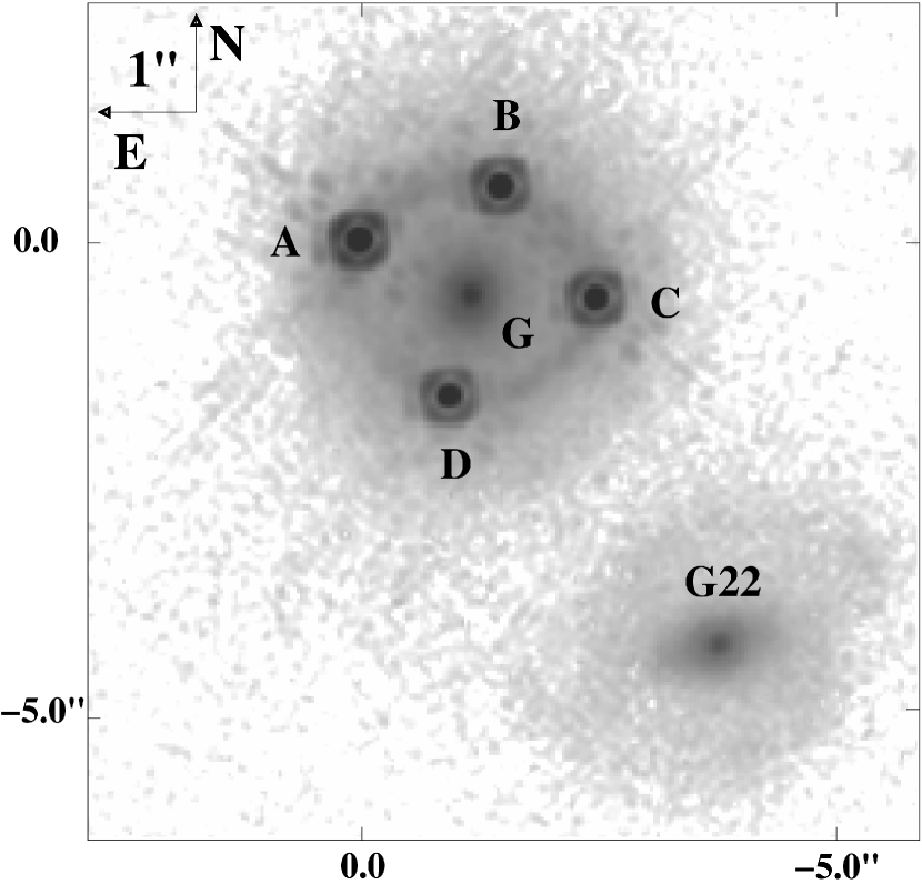
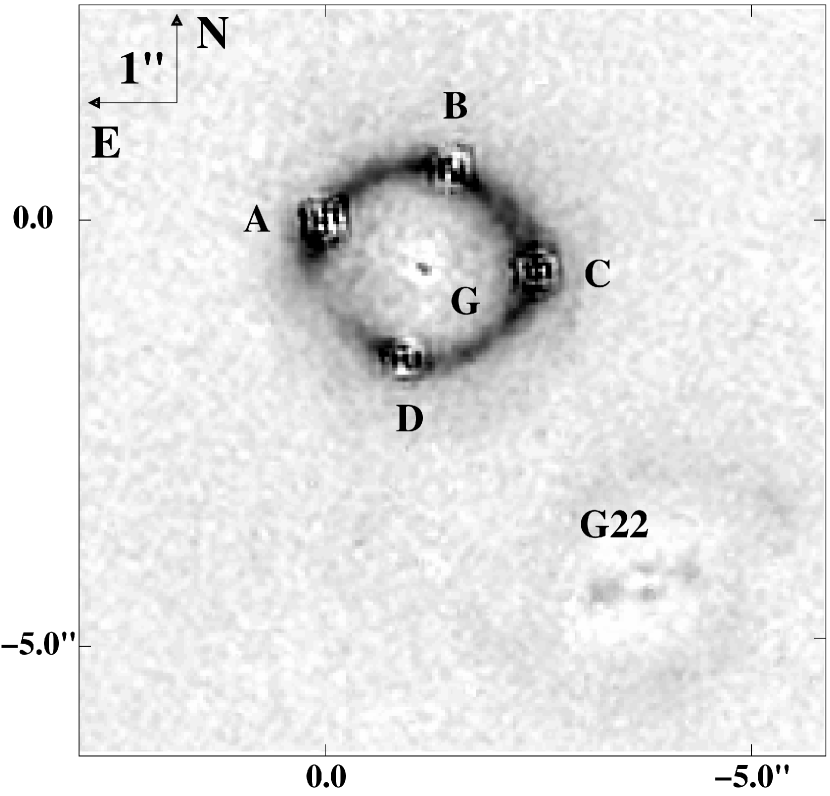
Figure 1: The gravitational lens HE 0435–1223 as observed with HST/NICMOS in the H-band. The top panel shows the original image. The bottom panel shows the residuals after subtracting a model of the 4 quasar images A–D, the lens galaxy G, and the neighboring galaxy G22. Within about $0\farcs 2$ of each quasar image position are subtraction artifacts due to imperfections of the PSF model.

The colors of the lens galaxy are in agreement with the predictions of standard population synthesis models for early-type galaxies in which star formation occurred at $z>1$. Using a range of such models to model the full spectral energy distribution of the lens galaxy and its evolution, we estimate that the rest-frame B-band absolute magnitude of the galaxy is $M_{B}=-20.46\pm 0.13$ mag (using $H_{0}=100$ km s^-1 Mpc^-1) and that it will evolve to an absolute B-band magnitude of $M_{B}=-20.3\pm 0.2$ mag at redshift zero. The neighboring galaxy G22 is bluer than the main lens galaxy, and its colors are better described by a model with a younger stellar population. Its rest-frame B-band luminosity is $M_{B}=-20.5\pm 0.5$ at the lens redshift, evolving to $M_{B}=-20.4\pm 0.5$ at redshift zero. The larger uncertainties than for the main lens galaxy are due to the broader range of evolution models consistent with the colors. In the model for the H-band image, the disk and the bulge of G22 have comparable fluxes of H$\simeq 18.8$ and $18.7$ respectively and scale lengths of $R_{d}\simeq 0\farcs 67\simeq 2.7h^{-1}$ kpc and $R_{e}\simeq 0\farcs 37\simeq 1.5h^{-1}$ kpc respectively.

The four quasar images have virtually identical colors, with the exception that image C seems to be redder by $0.17\pm 0.08$ mag in V$-$H than the other images. The colors of the quasar host galaxy (see “H” in Table 2) are consistent with those expected of an actively star-forming galaxy or from a galaxy that experienced a starburst at $z\simeq 2$. Using the method described by Kochanek, Keeton & McLeod (2000), we determined the closed curve that tracks the peak brightness of the Einstein ring as the azimuthal angle is varied from 0 to 2$\pi$ around the main lens galaxy. This curve is used as a modeling constraint in § 4.

3 Optical Monitoring

3.1 Observations and Data Reduction

The photometric monitoring observations took place between December 2003 and September 2005. Almost all of the data were obtained with the dual-beam ANDICAM camera (Depoy et al. 2003) mounted on the SMARTS 1.3m telescope, which is located at the Cerro Tololo Inter-American Observatory, in Chile. On each night, we obtained three 5 minute R-band exposures. We obtained simultaneous data in the J-band with ANDICAM, but we do not present any analysis of those data because of their much lower signal-to-noise ratio. A few observations were made with SPICAM on the 3.5m telescope of Apache Point Observatory (APO), in New Mexico. These APO observations consisted of three 1.5 min exposures in the Sloan Digital Sky Survey (SDSS) r-band at each epoch. For our final analysis, we retained only those images with a seeing of $1\farcs 8$ or better.

Although the data for this particular target were obtained with only two different telescopes (and are dominated by data from only one telescope), our monitoring campaign generally relies upon a broad array of different telescopes. For this reason, our data reduction pipeline was designed to cope with very heterogeneous images. The pixel scale, rotation, and other properties specific to the camera and telescope are stored in the image headers and accessed by the reduction pipeline. The basic idea underlying the pipeline is a version of PSF fitting. We perform a least-squares fit to each image, using a model with parameters that represent the quasar images, the lens galaxy, a set of comparison stars, the sky level, and the point spread function (PSF). The details are as follows.

For each target field, we define a set of subfields. One subfield encompasses the gravitational lens, and each of the others is centered on a comparison star. For the lens subfield, the model includes point sources for the template stars and quasar images, and an approximate de Vaucouleurs profile (see below) for the lens galaxy, all of which are convolved with the PSF. For HE0435–1223, the nearby galaxy G22 lay outside the modeled region. We hold fixed the relative positions of the quasar images and the structural parameters of the lens galaxy (i.e. its effective radius, axis ratio, and position angle), based on the parameters derived from HST  images. For the comparison star subfields, the model is a point source convolved with the PSF model. In addition, each subfield is given an independent sky level.

The PSF model is a superposition of three elliptical Gaussian functions. The relative major axis widths of the three functions are held constant, but the ellipticity and orientation of each function is allowed to vary. We allow for spatial gradients in each of the PSF parameters. We flux calibrate the images by including a prior constraint on the fluxes of the comparison stars. The mean flux of the comparison stars will vary slightly between frames (because of differences between the flux ratios of the comparison stars in the prior and in the best fit to the data). These variations provide a simple means of checking for significant problems in the PSF models. In the rare cases when a comparison star proves to be significantly variable, then either the data from that star are discarded, or, if they are desired for the determination of PSF parameters, they are kept and assigned very large flux uncertainties. Subfields that contain saturated pixels or that lie too close to the edge of the chip are ignored.

The lens galaxies are modeled using a Gaussian approximation to a de Vaucouleurs profile, i.e., a combination of a small number of elliptical Gaussian functions that best fits the integrated light profile of the appropriate de Vaucouleurs function. The accuracy of the approximation is controlled by the number of Gaussian functions employed. In practice, a single Gaussian function is often sufficient, since the lens galaxy typically contributes only a small fraction of the total light of a lens system. The advantage of the Gaussian decomposition is that the convolution with the PSF model can be computed analytically, allowing for extremely rapid computation. The integrated flux of the lens galaxy is required to be constant across all epochs, with a value that provides the minimum $\chi^{2}$ when applied to the entire series of images. A single Gaussian component was sufficient for HE0435–1223.

For HE 0435–1223, a listing of the comparison stars and their properties is given in Table 3. The photometry for the four quasar images (A, B, C, and D) is given in Table The Time Delays of Gravitational Lens HE 0435–1223: An Early-Type Galaxy With a Rising Rotation Curve, along with the differential variability of the flux standards and the value of $\chi^{2}/N_{dof}$, as a measure of image quality and the success of the fitting procedure. The r-band data were adjusted to the R-band scale by assuming an offset of $0.032$ mag, which was estimated by comparing images in each filter that were taken at similar epochs. The quoted uncertainties in the best-fitting quasar fluxes were determined from the full covariance matrix, and therefore incorporate the uncertainty the PSF model (but not the uncertainty in the lens galaxy flux, which was held constant after the optimization described in the previous paragraph). In the subsequent analysis, the uncertainty in each point with $\chi^{2}/N_{dof}>1$ was enlarged until the value of $\chi^{2}/N_{dof}$ for that particular image was unity, in order to lower the statistical weight of the points that were derived from problematic images. The final light curves are plotted in Fig. 2.

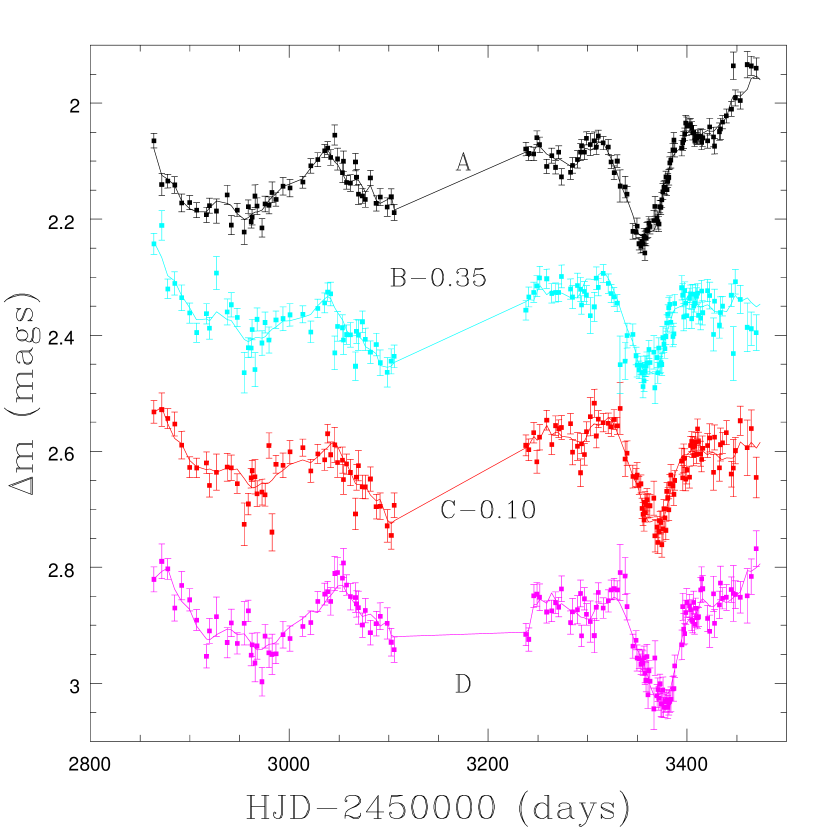
Figure 2: The light curves of images A, B, C, and D of HE 0435–1223. Arbitrary magnitude offsets have been applied to the B and C light curves, for display purposes. The solid lines are the best-fitting model light curves.

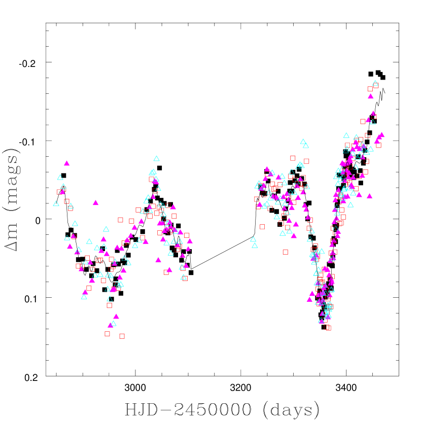
Figure 3: The time-shifted light curves of images A, B, C, and D of HE 0435–1223. The differential microlensing variations have been removed from the light curves of images B, C, and D. The solid line is the best-fitting model of the intrinsic variations of the source quasar. Error bars are not shown, to avoid clutter.

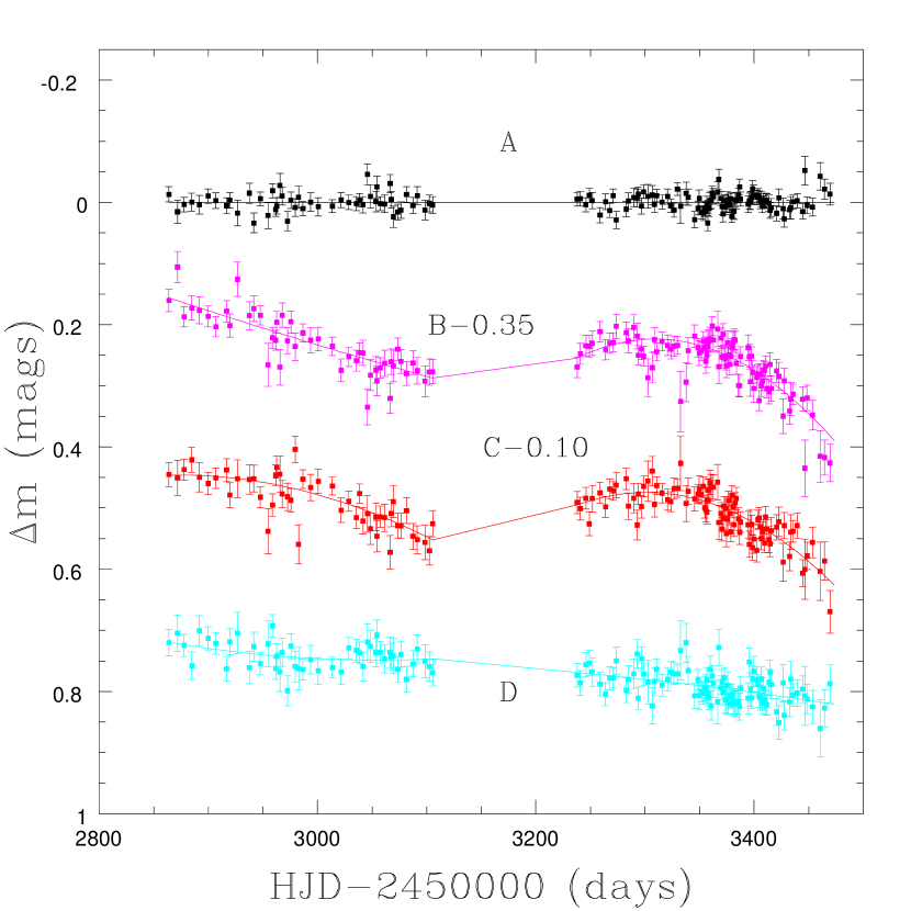
Figure 4: The differential microlensing light curves of images A, B, C, and D of HE 0435–1223, relative to image A. The best-fitting model of the intrinsic variations of the source quasar has been subtracted from the observed light curve of each image.

3.2 Light Curve Analysis

The patterns in the light curves that are common to all the images indicate that we have observed intrinsic variability at the level of 0.2 mag, which is highly significant when compared to our typical uncertainties of 0.01–0.02 mag. Less obviously, there are smaller-amplitude patterns that are specific to the light curve of each image. These uncorrelated patterns are the hallmarks of microlensing. Our goal was to decompose each light curve into intrinsic and the extrinsic variations, in order to estimate the differential time delays between the images and to analyze the microlensing variability.

We began with the premise that the intrinsic variations of the source quasar can be approximated as a Legendre series,

$$s(t)\simeq\sum_{m=0}^{N_{src}}a_{m}P_{m}\left[{t-t_{c}\over\delta t}\right],$$ (1)

where $s(t)$ is the magnitude of the source at time $t$, $t_{c}=(t_{N}+t_{1})/2$ is the midpoint of the time series, $\delta t=(t_{N}-t_{1})/2$ is the half-width of the time series, and $P_{m}$ is the $m$th Legendre polynomial. In the absence of microlensing, the light curve of the $i$th lensed image, $m_{i}(t)$, would be a time-shifted, magnified copy of the source light curve. To model the real light curves, we adopt image A as a reference image, and assume that the microlensing variations of each image relative to A can also be written as a Legendre series in time. Thus, $m_{i}(t)=s(t+\Delta t_{i})+\Delta\mu_{i}(t)$, where we have defined

$$\Delta\mu_{i}(t)=\sum_{m=0}^{N_{\mu}}c_{mi}P_{m}\left[{t-t_{c}\over\delta t}\right],$$ (2)

incorporating both the static magnification of the image and the differential microlensing variations. In fitting the observations $m_{ij}$ of the magnitude of image $i$ at time $t_{j}$, the ordinary fitting statistic is

$$\chi^{2}=\sum_{i=1}^{N_{im}}\sum_{j=1}^{N_{obs}}\left({m_{ij}-s(t_{j}+\Delta t_{i})-\Delta\mu_{i}(t_{j})\over\sigma_{ij}}\right)^{2}.$$ (3)

We cannot simply proceed by minimizing $\chi^{2}$, because any choice of the time delays would provide an acceptable fit if series of arbitrarily high orders were allowed. Some kind of restriction must be imposed that forces the model to exhibit “reasonable” quasar variability. Our approach, which is similar to that of Press, Rybicki & Hewitt 1992b , is to apply an a priori constraint that the intrinsic light curve has a power spectrum that is approximately the power spectrum of a “typical” quasar. Vanden Berk et al. (2004) have measured the typical quasar structure function in the r-band, using a large ensemble of quasar photometry from the SDSS, finding

$$V(\tau)=(\tau/\tau_{0})^{\gamma}\vspace{0.1in}{\rm mag}^{2}$$ (4)

with $\tau_{0}\simeq$ 70,000 days and $\gamma\simeq 1/3$. The $m$th term in our Legendre series has a mean square magnitude variation of $a_{m}^{2}/(2m-1)$ and a characteristic rest-frame time scale of $t_{m}=4\delta t/m(1+z_{s})$. Our “reasonability” constraint is that the mean squared power of each term should be $(t_{m}/\tau_{0})^{1+\gamma}$ (i.e. the root-mean-squared variations should vary as $m^{-4/3}$ for $\gamma=1/3$. Thus, instead of minimizing $\chi^{2}$, we minimize

$$H=\chi^{2}+\lambda\sum_{m=0}^{N_{src}}{a_{m}^{2}\over 2m-1}\left({\tau_{0}\over t_{m}}\right)^{1+\gamma},$$ (5)

where $\lambda$ is a Lagrangian multiplier that controls the weight of this a priori constraint on the quasar structure function relative to the weight of the individual data points. We determine the optimal values of $\Delta t_{i}$ by differentiating $H$ with respect to the parameters and solving the resulting linear equations. The data from each season are considered separately.

The task remains to choose the orders $N_{src}$ and $N_{\mu}$ of the Legendre series, and the strength of the Lagrange multiplier $\lambda$. In order to evaluate whether an increase in $N_{src}$ or $N_{\mu}$ is justified by the data, we use the F-test. We find that increasing $N_{src}$ results in a significant improvement until $N_{src}=20$ and thereafter ceases to be significant. Most of the improvement occurs in the range $5\leq N_{src}\leq 10$. As for the microlensing series, the improvement is significant as $N_{\mu}$ is increased to 3 and is not significant for larger choices. Most of the improvement occurs in the passage from $N_{\mu}=1$ (no microlensing) to $N_{\mu}=2$ (trends that are linear in time). We verified that these results do not depend strongly on the choice of $\lambda$, by comparing the cases $\lambda=0.01$ and $\lambda=1$.

In our final analysis, we adopted the values $N_{src}=60$, $N_{\mu}=3$, and $\lambda=1$. The choice of such a large value of $N_{src}$ should result in conservative uncertainties in the time delays. With these values, the longest delay is $\Delta t_{AD}=-14.37_{-0.85}^{+0.75}$ days, the intermediate delay is $\Delta t_{AB}=-8.00_{-0.82}^{+0.73}$ days and the shortest delay is $\Delta t_{AC}=-2.10_{-0.71}^{+0.78}$ days. The fractional uncertainties in the measurements are approximately 6%, 10%, and 35%, respectively. Fig. 3 shows the superposed light curves after shifting each light curve by the best-fitting time delay and subtracting the model of the differential microlensing variability. Table 5 Microlensing parameters for HE 0435–1223 gives the best-fitting parameters of the microlensing models for each season, and Fig. 4 shows the differential microlensing light curves. Relative to image A, image D has steadily faded. Meanwhile, images B and C faded more rapidly in the first season, then brightened between the two seasons, reached a peak during the second season and faded rapidly towards the end of the season. The common behavior of images B and C strongly suggests that it is actually image A that exhibits the greatest microlensing variability, although only the differential effects are observable.

As we would expect from an analysis of light curves that are short compared to a typical Einstein crossing time and show only low levels of variability, we cannot learn a great deal from the microlensing data as yet. We analyzed the microlensing light curves using the Monte Carlo method of Kochanek (2004) under the assumption that the average mass of the microlenses is within the range $0.2h^{2}M_{\odot}\leq\langle M_{*}\rangle\leq 2h^{2}M_{\odot}$. With this assumption, we do obtain a preliminary estimate for the physical size of the accretion disk: $0.8\mathrel{\raise 1.29167pt\hbox{$<$}\mkern-14.0mu\lower 2.58334pt\hbox{$\sim$}}r_{s15}\mathrel{\raise 1.29167pt\hbox{$<$}\mkern-14.0mu\lower 2.58334pt\hbox{$\sim$}}5.4$ where $r_{s15}=r_{s}/(10^{15}h^{-1}\hbox{cm})$. If we assume that the viscous energy release is radiated locally, then we can also estimate the ratio between the disk length scale $r_{s}$ and the gravitational radius $r_{g}=GM/c^{2}$ of the black hole to find that $r_{s}/r_{g}\simeq 39(L/L_{E})^{1/2}r_{s15}^{-1/2})$ for a black hole radiating with Eddington ratio $L/L_{E}$. Thus, our estimate of the disk scale length is a reasonable match to the hot, inner regions of an accretion disk. The data do not yet justify a more detailed microlensing analysis, but the prediction of all the microlensing models is that the future microlensing variability should be more dramatic than observed to date.

4 Models and Interpretation

4.1 Analytic theory

Kochanek (2002) presented an analytic theory of time delays that allows one to establish the quantitative connection between $H_{0}$ and the surface density of the lens galaxy, without any detailed lens modeling. It is based on a multipole-Taylor expansion of the lens potential (see also Trotter, Winn, & Hewitt 2000). In this section, we apply this theory to HE 0435–1223 in order to draw a few robust conclusions about the mass distribution of the lens galaxy.

For any pair of quasar images, we define $\langle\kappa\rangle$ as the mean surface density of the lens galaxy within an annulus whose inner and outer radii are the locations of the quasar images. It is often convenient to refer to this quantity as the “annular” surface density. We further define $\eta$ as the logarithmic slope of the surface density within the annulus (i.e. $\kappa\propto R^{\eta-1}$). We emphasize that both $\langle\kappa\rangle$ and $\eta$ are fundamentally local quantities, by which we mean that they describe the mass distribution over the very small range of radii that is spanned by the quasar images. Considering the pair of images for which the time delay is largest (and hence the fractional uncertainty in the time delay is smallest), and applying the procedure of Kochanek (2002), we find

$$H_{0}=(193\pm 25)(1-\langle\kappa\rangle)-(23\pm 3)\langle\kappa\rangle(\eta-1)\hskip 3.61371pt\hbox{km s}^{-1}~{}\hbox{Mpc}^{-1}.$$ (6)

This expression enforces a relation between $\eta$ and $\langle\kappa\rangle$, for a given value of $H_{0}$. For example, assuming that $H_{0}=(72\pm 7)$ km s^-1 Mpc^-1, and that the mass distribution of the lens galaxy is isothermal within the annulus ($\eta=2$), we may conclude that $\langle\kappa\rangle\simeq 0.56\pm 0.06$. If instead $\eta=3$ (a steeper mass distribution), then the surface density must be somewhat smaller: $0.51\pm 0.06$. Likewise, for the case $\eta=0$ (a shallower mass distribution), the surface density must be somewhat larger: $0.63\pm 0.06$.

Through this analysis, we see immediately that HE 0435–1223 is unlike most of the other simple, isolated time-delay lenses. Analyses of those other systems have shown that the lens galaxies are compatible with $H_{0}=(72\pm 7)$ km s^-1 Mpc^-1 only if their annular surface densities are considerably smaller than 0.5. For example, the lens galaxy of PG 1115+080 must have $\langle\kappa\rangle\simeq 0.24\pm 0.11$ near its Einstein radius. In contrast, the surface density of HE 0435–1223 at its Einstein radius is apparently larger than 0.5. An alternate way to express this result is that the lens galaxy of HE 0435–1223 has a slightly rising rotation curve, whereas the other lens galaxies have falling rotation curves.

Kochanek (2002) also showed how to use the astrometry and the time delay ratios to analyze the angular structure of the lens potential, and in particular to determine the balance between internal and external sources of shear. The “internal quadrupole fraction” $f_{\rm int}$ is defined such that a pure external shear has $f_{\rm int}=0$, an isothermal ellipsoid has $f_{\rm int}=0.25$, and an ellipsoidal mass distribution that is contained completely within its Einstein ring has $f_{\rm int}=1$. In this case we find that the angular structure is dominated by the external shear. As estimated from the astrometry, $f_{\rm int}=0.14\pm 0.04$. This agrees well with the estimate based on the time delay ratios, which is $f_{\rm int}=0.18\pm 0.04$.

4.2 Parametric Lens Modeling

In this section and the few sections to follow, we present a suite of calculations using traditional parametric lens models, in order to answer more specific questions about the mass distribution of the lens galaxy, the neighboring galaxies, and the possible presence of a group halo that envelops the galaxies. Whenever the results of these models can be compared to the analytic theory presented in the previous sections, they agree within about 10%.

Our goal is to identify models that successfully describe the positions of the quasar images relative to the lens galaxy, the Einstein ring curve formed by the quasar host galaxy, and the measured time delays. As a very conservative estimate of the uncertainties in the relative time delays, we doubled the statistical uncertainties that were presented in § 3.2. We fit the positions of the quasar images, the lens galaxy and the Einstein ring curve using lensmodel (Keeton 2001a ).

We used a three-component model, in which the components are the primary lens galaxy G, the nearby galaxy G22, and an independent external shear. We used a weak a priori constraint on the axis ratio of the G model ($q=0.74\pm 0.10$), which is intended to match the axis ratio of the surface brightness distribution measured with HST. We also used an a priori constraint on the amplitude of the external shear ($\gamma=0.05\pm 0.05$) based on limits from the alignment between the major axes of lens models and observed lens galaxies (Kochanek 2002). Ultimately we found that these a priori constraints did not play a significant role in determining the results. The a priori constraint on the Hubble constant was $H_{0}=72\pm 7$ km s^-1 Mpc^-1. We first described G with an ellipsoidal pseudo-Jaffe model [$\rho\propto r^{-2}(r^{2}+a^{2})^{-1}$]. In this model, the break radius $a$ can be varied continuously, allowing the mass distribution to be adjusted from the limit of a point mass ($a\rightarrow 0$) to the limit of an isothermal mass distribution ($a\rightarrow\infty$). We described G22 as either a point mass, a singular isothermal sphere (SIS), a singular isothermal ellipsoid (SIE), or a pseudo-Jaffe model.

In the best-fitting model, the mass of the lens galaxy within the cylinder bounded by the Einstein ring ($b=1\farcs 18=4.8h^{-1}$ kpc) is $2.2\times 10^{11}hM_{\odot}$. As always, this is the most robust result of lens modeling, with a negligible statistical uncertainty. The corresponding velocity dispersion for an SIS model is $\sigma=255$ km s^-1. The best-fitting value of the break radius is $a\rightarrow\infty$, so the best-fitting pseudo-Jaffe mass distribution for G is essentially isothermal. The lower limit on the break radius is $a>14\farcs 7=59h^{-1}$ kpc at 1$\sigma$ confidence, and $a>5\farcs 4=22h^{-1}$ kpc at 2$\sigma$ confidence. These constraints are illustrated in Fig. 6, which shows how the goodness-of-fit parameter ($\chi^{2}$) varies with the choice of break radius. (Also plotted in Fig. 6 are the results from the group-halo models discussed in § 4.4.) The requirement that the model match the observed time delays leads to the constraint on the break radius.

Notably, even in the best-fitting model, in which the mass distribution has a nearly flat rotation curve, the fit is rather poor ($\chi^{2}_{\rm delay}\simeq 7$ for $a=40\farcs 0$). One way to state the difficulty is that the favored value of the Hubble constant is $H_{0}\simeq 94$ km s^-1 Mpc^-1, as compared to the constraint of $H_{0}=72\pm 7$ km s^-1 Mpc^-1. Since the time delays of the model scale as $\Delta t\propto(1-\langle\kappa\rangle)/H_{0}$, it follows that a better fit would be obtained if $\langle\kappa\rangle$ were allowed to be larger than 0.5, i.e., if the rotation curve of the galaxy were rising rather than flat.

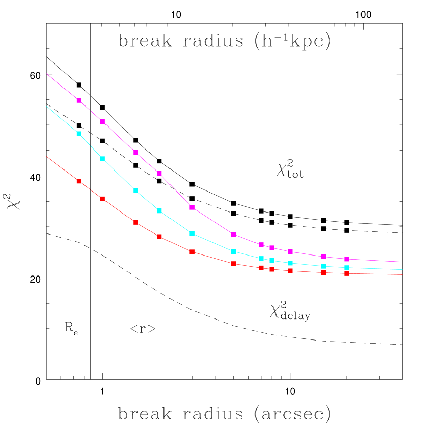
Figure 5: (Left) The goodness-of-fit parameter as a function of $a$, the break radius of the pseudo-Jaffe model for the lens galaxy G. The break radius is the length scale at which the rotation curve of the galaxy undergoes a transition from flat to Keplerian. The uppermost solid curve is for a model with an external shear. The next three solid curves are for models in which the lens galaxy is embedded in a group NFW halo with a break radius of either $r_{c}=20\farcs 0$, $10\farcs 0$ or $5\farcs 0$ (from top to bottom). The uppermost dashed curve shows the result when the group halo is modeled as an SIS. The variation in $\chi^{2}$ is governed mainly by the constraint on the observed time delays; this is illustrated by the lower dashed curve, which shows $\chi^{2}_{\rm delay}$ for the external shear model. The vertical lines mark the mean radius of the quasar images, and the effective radius of the lens galaxy.

Figure 6: (Right) The environment of HE 0435–1223. The 5 squares near the center of the map show the positions of the lens galaxy and the 4 quasar images. The large circles centered on the lens are the $20\farcs 0$ and $40\farcs 0$ radii, for visual reference. The small circles mark the locations of nearby galaxies that were identified by Morgan et al. Morgan2004p00 (2004), and the sizes of each circle are proportional to the expected amplitude of the lensing perturbation from that galaxy. Solid circles are for external shear, and dashed circles are for higher-order perturbations. The line between the lens galaxy and G20 is the locus of allowed positions for the centroid of a group halo.

4.3 The Effect of the Lens Galaxy Environment

Before considering further changes in the radial structure of the lens galaxy, we explore the possible influences of the lens galaxy environment on the measured quantities. Fig. 6 is a map of the lens galaxy and its closest neighbors, in which the symbol sizes encode the relative strengths of the perturbations expected from each galaxy. In creating this map, we assumed that the Einstein radius of each galaxy was proportional to the square root of its I-band luminosity ($b_{i}\propto\sigma_{i}^{2}\propto\sqrt{L_{i}}$). The amplitude of the external shear is then expected to be proportional to $(b_{i}/R_{i})$, and higher-order perturbations are proportional to $(b_{i}b/R_{i}^{2})$, where $b$ is the Einstein radius of the lens galaxy and $R_{i}$ is the angular separation from the lens galaxy. The dominant perturbation comes from G22, as it is both nearby and fairly luminous.

We cannot detect the external shears produced by individual galaxies because they are degenerate with the global external shear – the effect of an individual galaxy can be detected only through higher-order perturbations. As shown in Fig. 8, the higher-order perturbations generated by G22 are measurable and correspond to a constraint on its shear of $\gamma_{{\rm G}22}=0.025\pm 0.008$, regardless of whether G22 is modeled as an SIS or a point mass, and regardless of the structure of the main lens galaxy G. When G22 is modeled as an SIS, the best-fitting Einstein radius is $0\farcs 22\pm 0\farcs 07$, corresponding to a circular velocity $v_{c}=157\pm 25$ km s^-1. Since G22 should have negligible surface density at projected radii corresponding to the $R_{{\rm G}22}\simeq 4\farcs 4\simeq 18h^{-1}$ kpc projected separation of G22 and the lens, the shear that is produced by G22 equals the mean surface density of interior to $R_{{\rm G}22}$. In short, the mass of G22 can be estimated from the higher order perturbations it produces, and the result is $M_{{\rm G}22}(R<R_{{\rm G}22})=(7.9\pm 2.6)\times 10^{10}hM_{\odot}$.

As discussed by Morgan al. Morgan2004p00 (2004), we can use this measurement of the mass of G22 to determine whether or not this companion galaxy possesses a dark matter halo. Based on our estimate of the evolution-corrected B-band luminosity of G22 and the B-band Tully-Fisher relations of Kannappan, Fabricant & Franx (Kannappan2002p2358 (2002)), G22 should have a circular velocity of $v_{c}\simeq 190\pm 45$ km/s. This is very close to the circular velocity of $v_{c}=150\pm 25$ km s^-1 predicted for G22 assuming an SIS mass distribution and the measured critical radius. Since the lens model constrains the mass $M_{{\rm G}22}(R<R_{{\rm G}22})$, the predicted circular velocity depends only the scale length $R_{d}$ of G22’s mass distribution, $v_{c}^{2}\propto M_{{\rm G}22}(R<R_{{\rm G}22})/R_{d}$. As we make the mass distribution of G22 more compact (smaller $R_{d}$), then we predict a higher circular velocity. If we use our best fit disk plus bulge model from the HST data as a constant-$M/L$ model for the mass distribution, then we predict $v_{c}\simeq 275$ km s^-1, while if we add a standard NFW halo normalized so that the stars represent only 15% of the mass, we predict $v_{c}\simeq 180$ km s^-1. Thus, if the Tully-Fisher estimate of the circular velocity is correct, G22 must have a significant dark matter halo.

Unfortunately, we find that this same technique cannot be used to learn much about the other neighboring galaxies, because the perturbations that they produce are too small. The next-largest perturbation comes from the close pair of galaxies G12 and G21, which together should produce higher-order perturbations that are only 40% of strength of the effect of G22. We computed a series of models in which G21 was represented as an SIS, in addition to G22. The result was a small improvement in the fit, and a best-fitting Einstein radius for G21 of $b_{{\rm G}12}=0\farcs 17$ (or, equivalently, $\gamma_{{\rm G}12}=0.008$ and $M_{{\rm G}12}(R<R_{{\rm G}12})=1.0\times 10^{11}hM_{\odot}$, where $R_{{\rm G}12}=8\farcs 9=36h^{-1}$ kpc is the projected separation of G12 and G). But the uncertainties are large enough that at at $1\sigma$ confidence we can place only upper bounds of $b_{{\rm G}12}<0\farcs 28$, $\gamma_{{\rm G}12}<0.02$, and $M_{{\rm G}12}(R<R_{{\rm G}12})<2.5\times 10^{11}hM_{\odot}$. Given the large uncertainties, it is fruitless to try to distinguish the effects of G12 and G21 separately.

We also tried models that incorporated an a priori constraint on the external shear, $\gamma=0.00\pm 0.01$, thereby requiring that the angular structure of the lens potential be determined entirely by the primary lens galaxy and the SIS model components representing neighboring galaxies. We included SIS components for all the observed galaxies within 20″. We further assigned weak priors (50% accuracy) that encouraged the Einstein radii of the SIS models to agree with the estimates based on the observed I-band luminosities. The resulting fits to the data were only slightly poorer than the cases in which the external shear was allowed to vary independently. We conclude that the nearby galaxies are sufficient to explain most of the angular structure in the lens potential, but that there is a small component ($\gamma_{\rm ext}\simeq 0.01$ with a position angle of about $-20^{\circ}$) that is not easily attributable to the nearby galaxies. This is a reasonable result, in light of previous work that has shown that large-scale structure along the line of sight should generally provide a contribution to the shear that is of this order of magnitude (e.g. Barkana Barkana96 (1996)). Similar results were obtained when we enlarged the sample of SIS galaxies to include all the observed galaxies within 40″.

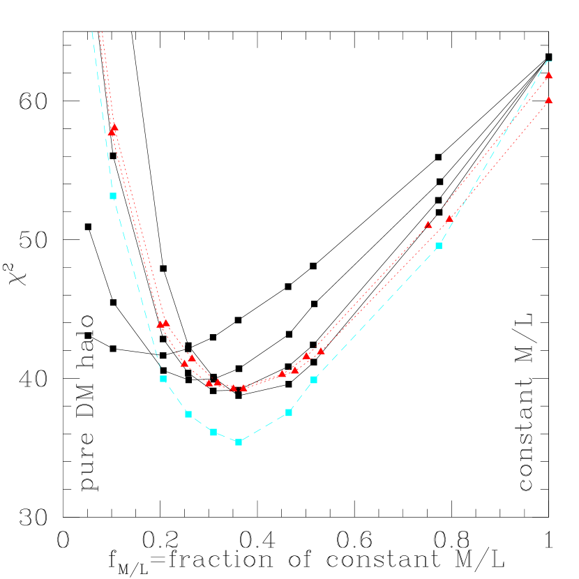
Figure 7: (Left) The goodness-of-fit parameter is plotted as a function of the shear $\gamma_{\rm pert}$ induced by the neighboring galaxy G22. Although parametrized by the shear, the constraints are due to the higher order perturbations produced by G22 – the shear itself is degenerate with the global, external shear included as part of the model. Results are shown for cases in which G22 is described by an SIS (solid squares), SIE (open squares), and a pseudo-Jaffe model with a break radius of $a=1\farcs 0$ (dashed, filled triangles). In all of these cases, the main lens galaxy is described as a pseudo-Jaffe model with $a=10\farcs 0$. If instead $a=2\farcs 0$ for the main galaxy, the Einstein radius of the SIS model for G22 increases slightly (dotted, pentagons).

Figure 8: (Right) Results of “galaxy plus halo” (de Vaucouleurs plus NFW) models. The goodness-of-fit parameter is plotted as a function of $f_{M/L}$, which is the mass of the de Vaucouleurs component divided by the mass of the best-fitting pure-de Vaucouleurs model. The 4 solid curves with squares show models with $R_{e}=0\farcs 86$ and $r_{c}=2\farcs 5$, $5\farcs 0$, $10\farcs 0$ and $20\farcs 0$ (in increasing order of the optimum value of $f_{M/L}$). The dashed line with squares shows the results for the case in which $R_{e}=0\farcs 86$ and the NFW halo shape is allowed to vary freely (as opposed to being constrained by the observed surface brightness distribution). The dotted curves with triangles show the results for $R_{e}=1\farcs 0$ and $1\farcs 2$ with $r_{c}=10\farcs 0$.

4.4 The Possibility of a Group Halo

It is possible that the mass distribution is better described by a single “group halo” rather than by individual SIS components at the locations of all the observed galaxies. However, models in which the centroid of the group halo do not coincide with the position of a galaxy are not theoretically popular – for example, models of the halo occupancy distribution (HOD) argue that all halos have a central galaxy and that the central galaxy is generally the most massive (e.g. Cooray & Sheth Cooray02 (2002)). In the models described in § 4.2 (consisting of a primary lens, the perturber G22, and an external shear) the external shear has an amplitude of $\gamma\sim 0.05$ and a position angle of approximately $-30^{\circ}$. Morgan et al. (2004) provided some evidence that the centroid of the galaxy group is in that general direction. We explored for this possibility by replacing the independent external shear parameter with a mass component representing a group halo. We tried both an SIS and an NFW mass distribution to describe the group halo. The results are plotted in Fig. 6 along with the previously described results for the external-shear models.

Generally speaking, the group-halo models provide a better fit to the data than the external-shear models. Within the group-halo models, those that have a higher convergence (for a fixed shear) produce better fits. The extra convergence allows a better fit to the time delays. Consequently, an NFW halo is favored over an SIS halo, and large NFW break radii are favored over small NFW break radii. Regardless of the form of the group-halo model, the data still impose a strong constraint on the break radius of the primary lens galaxy. The $2\sigma$ lower limit on $a$ is $4\farcs 9$ for an SIS group halo. For an NFW group halo, the corresponding lower limits are $3\farcs 4$, $4\farcs 7$, and $6\farcs 4$, for an NFW break radius of $20\farcs 0$, $10\farcs 0$, and $5\farcs 0$, respectively.

The best-fitting centroid positions for the group halo do not seem to be associated with any of the observed galaxies (see Fig. 6), which may be unphysical. The key property of the group-halo models that accounts for their superior fit to the data is that they are allowed the freedom to contribute to the local surface density near the primary lens galaxy, unlike the external-shear models. In fact, if there were a massive group halo, one would expect the primary lens galaxy to lie at its center, since the primary lens galaxy is the most luminous galaxy in the field. Its Einstein radius is nearly 5 times larger than that of the second-place galaxy G22, and its luminosity is nearly 4 times that of G22.

4.5 Embedding the Lens Galaxy in a Dark Matter Halo

All of the the preceding calculations have suggested that a concordance between $H_{0}=(72\pm 7)$ km s^-1 Mpc ^-1 and the measured time delays of HE 0435–1223 requires that the primary lens galaxy should have a rising rotation curve. Even our SIS models for G did not have a large enough surface density at the location of the Einstein radius to be compatible with the accepted value of $H_{0}$.

In order to build a model with a rising rotation curve, we combined a constant-$M/L$ model with an NFW halo. For the constant-$M/L$ component (the “galaxy” or “stellar component”), we considered models in which the galaxy has an effective radius of $R_{e}=0\farcs 86$, $1\farcs 0$ or $1\farcs 2$. We constrained its axis ratio to be $0.79\pm 0.04$, and the position angle of its major axis to be $-5^{\circ}\pm 4^{\circ}$, to match the observed surface brightness distribution. For the NFW component (“halo”), we considered four different values of the break radius: $r_{c}=2\farcs 5$, $5\farcs 0$, $10\farcs 0$ and $20\farcs 0$. The halos were centered on the stellar mass distribution and were generally constrained to have the same ellipsoidal shape. (Experiments in which the halo shape was allowed complete freedom did result in slightly improved fits, but did not change any of the conclusions described below about the radial mass distribution.) Since only G22 produces significant higher-order perturbations beyond an external shear, we included an SIS component representing G22. The cumulative effect of all the other galaxies (and large-scale structure) was represented by an external shear.

The results of these models are shown in Fig. 8. The variation in the goodness-of-fit parameter $\chi^{2}$ is plotted as a function of $f_{M/L}=M_{\star}/M_{\star,{\rm nohalo}}$. This dimensionless factor is proportional to the mass of the stellar component. It has been divided by the mass of the stellar component in the best-fitting model with no NFW halo (a purely constant-$M/L$ model). The $\chi^{2}$ values in this plot cannot be directly compared to those in Fig. 6, because of the additional constraints on the shape of the stellar mass distribution that we are imposing in this case.

The results can be summarized as follows:

1. Neither a constant-$M/L$ model, nor a pure-halo model, can provide an acceptable fit to the data. These two extremes can be ruled out with high confidence.

2. The best-fitting value of $f_{M/L}$ has a weak dependence upon the scale lengths of the mass components. For an effective radius of $R_{e}=0\farcs 86$, and NFW break radii of $r_{c}=2\farcs 5$, $5\farcs 0$, $10\farcs 0$, and $20\farcs 0$, we find $f_{M/L}=0.18\pm 0.10$, $0.28\pm 0.08$, $0.34\pm 0.07$ and $0.39\pm 0.07$, respectively. This dependence can be understood as the necessity for $f_{M/L}$ to increase as the break radius increases, in order to maintain a fixed surface density near the Einstein ring. Similarly, if we hold $r_{c}=10\farcs 0$ fixed, and make the galaxy less centrally concentrated with the choice $R_{e}=1\farcs 0$, then $f_{M/L}$ increases correspondingly to $0.36\pm 0.08$.

3. All of the best-fitting models agree on the value of the surface density within the annulus bounded by the images: $\langle\kappa\rangle\simeq 0.60\pm 0.05$. As explained in § 4.1, it is this quantity that controls the connection between the observed time delays and the Hubble constant. Note that this value of $\langle\kappa\rangle$ agrees well with the simple analytic estimate of §4.1, is 20% larger than SIS value of 0.5, and is much larger than the constant-$M/L$ value of 0.22.

4. If the effective radius of the stellar component is held fixed, then $\langle\kappa_{\star}\rangle$ (the stellar surface density at the Einstein radius) is correlated with the NFW break radius, in the sense that more compact halos must be more dark-matter dominated. For example, if $R_{e}=0\farcs 86$, then $\langle\kappa_{*}\rangle\simeq 0.05\log(hr_{c}/\hbox{kpc})$. Again, this can be understood as the necessity to maintain a sufficiently high total surface density near the locations of the quasar images.

5. Fig. 9 shows the deflection profiles of the best-fitting models with both NFW and constant-$M/L$ components. The deflection profile is roughly equivalent to the square of the rotation curve. At the location of the Einstein radius, the deflection profiles are increasing functions of radius, i.e., the galaxy has a slightly rising rotation curve.

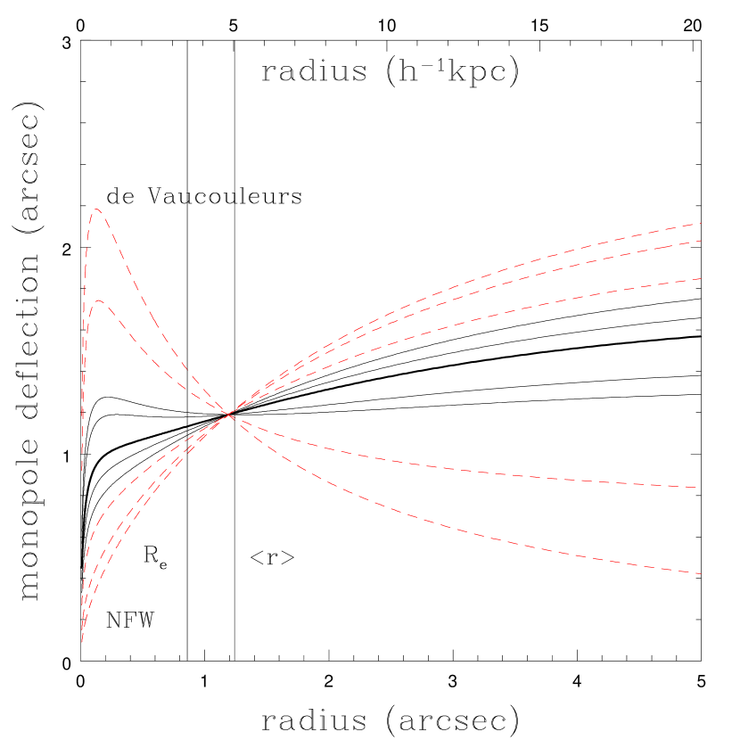
Figure 9: Radial deflection profiles for the “galaxy plus halo” (de Vaucouleurs plus NFW) models, with $R_{e}=0\farcs 86$ and $r_{c}=10\farcs 0$. The heavy solid curve is the best-fitting model and the light solid curves are models that also provide an acceptable fit ($\Delta\chi^{2}<4$). The deflection profiles plotted here are approximately the square of the rotation curve. The best fitting pseudo-Jaffe models have a constant deflection profile (flat rotation curve). A constant-$M/L$ (de Vaucouleurs only) model has a falling rotation curve and results in a poor fit to the data. The vertical lines mark the effective radius $R_{e}$ and the mean radius of the images $\langle r\rangle$.

These results from the lens models are supported by estimates of the mass-to-light ratio of the galaxy. The mass of the galaxy within its Einstein radius is determined from the measured redshifts and astrometry, without appreciable systematic error. Given the estimated B-band luminosity of the galaxy (§ 2), we can estimate the mass-to-light ratio of all the material within the Einstein radius. For the measured value $R_{e}=0\farcs 86$, the luminosity within the Einstein radius is 58% of the total luminosity. Putting it all together, the implied B-band mass-to-light ratio within the Einstein ring is $\Upsilon_{B}=15.6\pm 1.9$ as observed, and $\Upsilon_{B}=19.0\pm 4.2$ when corrected for evolution to redshift zero. (The uncertainties are dominated by the uncertainty in the luminosity.) Given the local estimate of $\Upsilon_{*}=7.8\pm 2.7$ by Gerhard et al. Gerhard2001p1936 (2001), the implication is that stars represent only $(40\pm 17)$% of the mass projected inside the Einstein ring, which is consistent with the results of the lens models.

4.6 The Connection to Theoretical Halo Models

In order to connect these models to theoretical expectations we must relate the halo parameters to estimates from simulation and account for the changes in the dark matter distribution produced by they baryonic component known as “adiabatic compression” (Blumenthal et al. Blumenthal86 (1986)). In principle, we could use adiabatically compressed halos in the lens modeling, but in practice it would slow down the computations by an unacceptable degree because of the need for ellipsoidal rather than circular lens models. Recall, however, that the data really only specify the mass within the Einstein ring and the surface density at the ring. With this in mind, we searched for adiabatically compressed halo models that match these key observables. For each of the “galaxy plus NFW” models described in the previous section, we calculated the mass within the Einstein radius and the surface density at the Einstein radius. As a matter of convenience, we used a Hernquist model (Hernquist Hernquist1990p359 (1990)) instead of the de Vaucouleurs model. Hernquist models have the desirable property that the enclosed mass as a function of radius can be computed analytically in both two and three dimensions. We then searched a collection of adiabatically-compressed halo models for examples that satisfy the constraints on the enclosed mass and the local surface density. The collection of halo models was the same collection that was computed previously by Kochanek Kochanek2003p49 (2003), which in turn was based upon the early-type lens models of Keeton 2001b and the Bullock et al. bullock2001p559 (2001) parameterizations of halo virial masses and concentrations.

First, we consider halos without applying any adiabatic compression. Fig. 10 shows the ability of these models to fit the data, as a function of the halo concentration and the cold baryonic mass fraction $f_{b,{\rm cold}}$. The latter quantity represents the stellar component. In a constant-$M/L$ model, $f_{b,{\rm cold}}=1$, but in a standard CDM halo it is limited to the global baryonic mass fraction of $f_{b,{\rm cold}}<0.15=\Omega_{b}/\Omega_{\rm M}$ (Spergel et al. Spergel2003p175 (2003)). The range of NFW break used in the models of §4.5 span the range that i s expected for a halos with the mass of the primary lens galaxy. The models which successfully fit the data have relatively low baryon fractions, $\log f_{b,{\rm cold}}=-2.3\pm 0.4$ compared to the global average, so only $\sim 3\%$ of the baryons originally in the halo can have cooled to make the observed galaxy. The best-fitting halos have a virial mass of $\log(M_{vir}/hM_{\odot})=13.5\pm 0.4$, a virial radius of $\log(hr_{vir}/\hbox{kpc})=2.7\pm 0.1$, and a break radius of $\log(hr_{c}/\hbox{kpc})=2.0\pm 0.3$. The mass of the stellar component is $\log(M_{*}/hM_{\odot})=11.2\pm 0.2$. The contribution from dark matter is considerable even within the Einsten radius. In projection, the stars constitute $(40\pm 10)\%$ of the mass inside the Einstein radius and $(30\pm 8)\%$ of the mass within two effective radii. In three dimensions, the stars constitute $(74\pm 11)\%$ of the mass inside a sphere with a radius of $R_{e}$. Thus, measurements of stellar dynamics through optical spectroscopy would be mainly sensitive to the stellar mass rather than the dark matter.

Next, we include the effects of adiabatic compression. The dark matter becomes more important, and the inferred stellar surface density must be adjusted to compensate. We express this by parameterizing the results as a function of the ratio of stellar surface densities found with and without adiabatic compression. Fig. 10 also shows the effect of adding adiabatic compression to the models. The cold baryon fraction $\log f_{b,{\rm cold}}=-2.4\pm 0.4$ and the stellar mass $\log(M_{*}/hM_{\odot})=10.9\pm 0.2$ are a factor of two smaller, but the virial mass, virial radius, and break radius are little changed. As a result, the dark-matter fraction in the inner regions rises appreciably, to $(77\pm 9)\%$ and $(82\pm 10)\%$ of the projected mass inside the Einstein radius and $2R_{e}$, and to $(58\pm 8)\%$ of the mass inside a sphere of radius $R_{e}$.

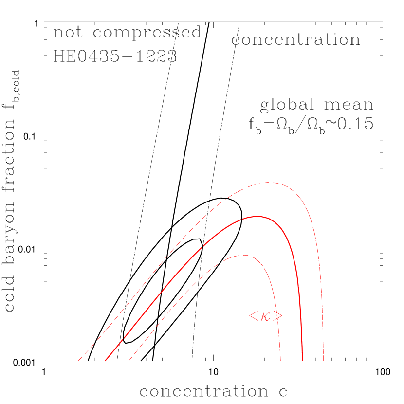
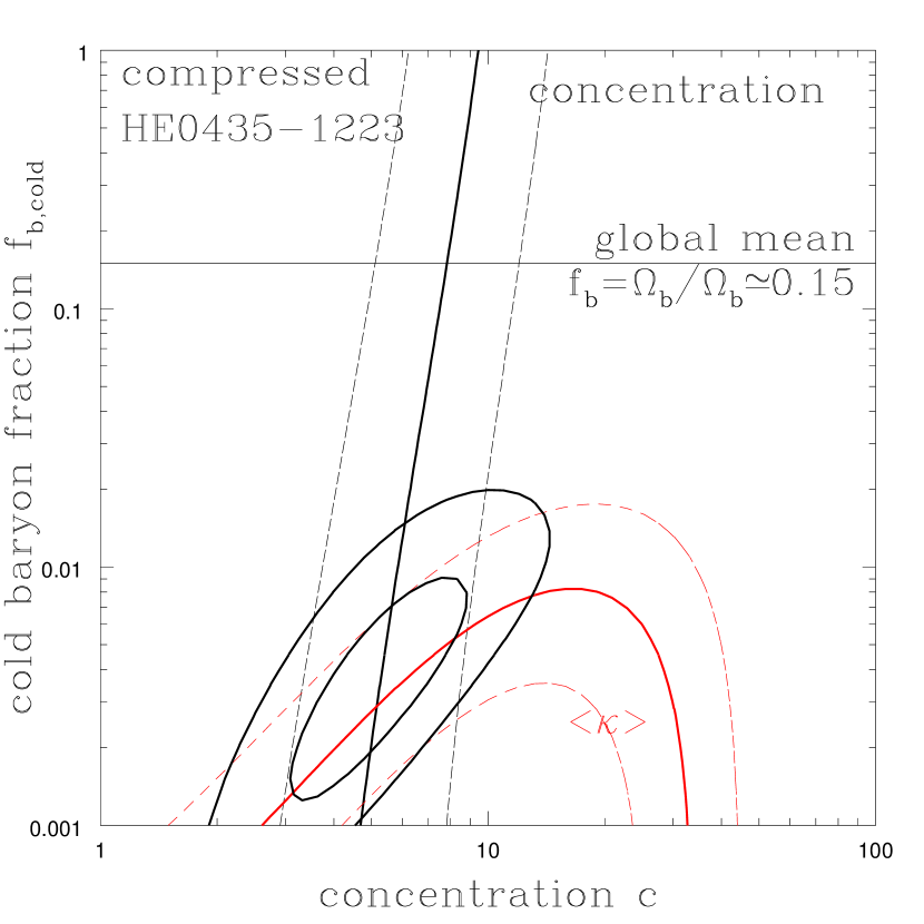
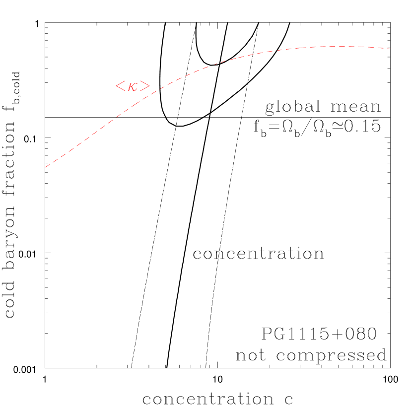
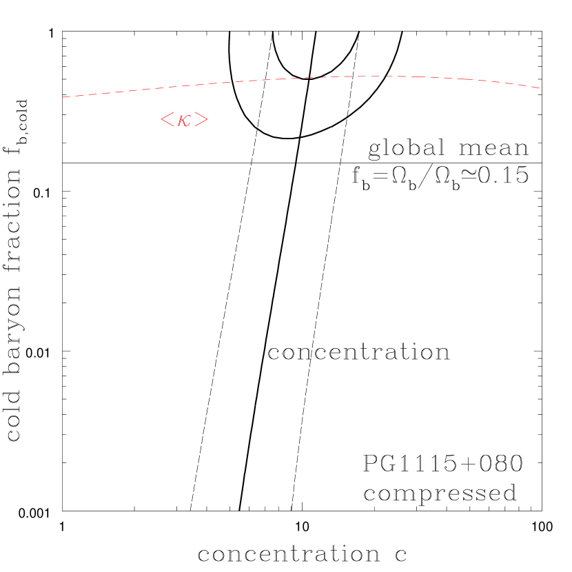
Figure 10: Standard halo models for HE 0435–1223 (top) and PG 1115+080 (bottom), without adiabatic compression (left) and with adiabatic compression (right). The error ellipses show the 68% and 95% confidence regions in the space of the halo concentration $c$ and the cold baryon fraction $f_{b,{\rm cold}}$. The constraint is essentially the product of the constraint on the halo concentration for a given halo mass (roughly vertical solid and dashed lines showing the mean and typical dispersion in the concentration) and the surface density at the Einstein ring $\langle\kappa\rangle$ (the second set of solid and dashed lines). For PG1115+080, only the lower bound on $\langle\kappa\rangle$ is visible. A horizontal line marks the global mean value for the ratio between the baryonic and total masses of halos.

5 Conclusions

Our analysis of HE 0435–1223 adds to the evidence that the structures of early-type galaxy halos are heterogeneous, rather than homogeneous. Assuming that $H_{0}=(72\pm 7)$ km s^-1 Mpc^-1, most time-delay lens galaxies must have centrally concentrated mass distributions that are strongly dominated by the stars in their central regions (Kochanek 2002). They must have falling rotations curves and low surface densities at the galactocentric distances where the lensed images occur (1–2$R_{e}$). HE 0435–1223, by contrast, must have a rising rotation curve at the radius of the lensed images. As an illustration of this heterogeneity, we performed the same “galaxy plus NFW” analysis for the quadruple-image quasar PG 1115+080. In that case, the best-fitting model has constant mass-to-light ratio ($f_{M/L}>0.9$), a very small surface density at the Einstein radius ($\langle\kappa\rangle=0.16\pm 0.05$), and a comparable stellar surface density. If we focus on the adiabatically-compressed model, then the estimated stellar mass in the PG 1115+080 model [$\log(M_{*}/hM_{\odot})=10.7\pm 0.1$] is similar to the estimate for HE 0435–1223, but the virial mass [$\log(M_{vir}/hM_{\odot})=10.9\pm 0.1$] is far smaller. This is because the cold-baryon fraction in the PG 1115+080 model is nearly unity. In fact, the cold-baryon fraction must be larger that the cosmological limit of $\Omega_{b}/\Omega_{\rm M}\simeq 0.15$.

The enormous difference between these halos is difficult to attribute to any errors in our measurements of HE 0435–1223. Our estimates for the surface densities can be incorrect only in the event of a gross error in the time delay measurements, or if there are contributions to $\langle\kappa\rangle$ besides the primary lens galaxy and its halo. The former possibility is very unlikely because of the multiple correlated features that we observed in the light curves of the four images. The latter possibility is also unlikely, given the results of the extensive suite of models presented in § 4. For example, models with $f_{b,{\rm cool}}\simeq 0.1$ have annular surface densities of $\langle\kappa\rangle\simeq 0.3$ rather than $0.6$, which would require a time delay of $\Delta t_{AD}\simeq-25$ days. This is ruled out at very high confidence. We attempted to find successful models in which some of the convergence was generated by a nearby group halo, but we found that these models cannot remove the requirement that the lens galaxy has a rising rotation curve; they produce too much shear.

A natural context in which this heterogeneity of halos might be understood is the halo model for populating dark matter halos with galaxies (see the review by Cooray & Sheth Cooray02 (2002)). The typical early-type lens galaxy should be a member of a group of galaxies. In the halo model, one of the galaxies in a group lies at the center of the massive group halo, while the other galaxies are smaller satellites orbiting in the group halo. Because baryonic cooling enormously increases the central densities of galaxies as compared to a pure dark-matter halo, the lensing cross section is dominated by the individual cross sections of the member galaxies, rather than the group as a whole (e.g. Kochanek & White Kochanek2001p531 (2001)). However, it is likely that the surface densities and stellar mass fractions of the central galaxy and the satellite galaxies on scales larger than an effective radius are very different.

In this context, one possible interpretation is that HE 0435–1223 is the central galaxy of its group. It has a high dark-matter surface density, and the stars constitute only a small fraction of the overall baryonic mass of the group. At the other extreme, the lens galaxy in PG 1115+080 is a satellite galaxy with a partially stripped halo all of whose baryons have been converted to stars. The galaxy G22 in HE 0435–1223 is intermediate to these extremes.

Which type of galaxy dominates the lens population: central galaxies, or satellite galaxies? The theoretical expectation is unclear. It depends on the detailed balance between the higher cross-section of the more massive central galaxies and the large number of satellite galaxies. The present sample of time delay lenses suggests the two populations are comparable. The three lenses PG 1115+080, HE 2149–2745 and B1600+434 require low dark-matter surface densities (for $H_{0}=72$ km s^-1 Mpc^-1) and are probably satellite galaxies. In contrast, HE 0435–1223 and HE 1104–1805 require high dark-matter surface densities, and are probably central galaxies of groups. This explanation for the heterogeneity of the time delay lenses predicts that for time delay lenses that are satellite galaxies, there should be a nearby, group center galaxy that has a much higher mass-to-light ratio than either the lens or other satellite galaxies.

Table 1: Astrometry of HE 0435–1223

Component	$\Delta\hbox{RA}$	$\Delta\hbox{Dec}$
A	$\equiv 0$	$\equiv 0$
B	$+1\farcs 476\pm 0\farcs 003$	$+0\farcs 553\pm 0\farcs 001$
C	$+2\farcs 467\pm 0\farcs 002$	$-0\farcs 603\pm 0\farcs 004$
D	$+0\farcs 939\pm 0\farcs 002$	$-1\farcs 614\pm 0\farcs 001$
G	$+1\farcs 165\pm 0\farcs 002$	$-0\farcs 573\pm 0\farcs 002$

Note. — For the NICMOS images we adopted pixel scales of $\Delta x=0\farcs 0760$ and $\Delta y=0\farcs 0753$.

Table 2: Photometry of HE 0435–1223

Comp	H=F160W	I=F814W	V=F555W	$R_{e}$	$\mu_{e}$	$q$	$\theta_{maj}$
	(mag)	(mag)	(mag)	(”)	mag/arcsec2		(PA, deg)
A	$17.31\pm 0.02$	$17.84\pm 0.02$	$18.41\pm 0.03$
B	$17.80\pm 0.02$	$18.39\pm 0.04$	$18.99\pm 0.07$
C	$17.80\pm 0.03$	$18.41\pm 0.02$	$19.07\pm 0.06$
D	$18.06\pm 0.02$	$18.62\pm 0.04$	$19.12\pm 0.04$
G	$16.86\pm 0.04$	$18.85\pm 0.02$	$21.55\pm 0.13$	$0\farcs 86\pm 0\farcs 04$	$18.26\pm 0.07$	$0.79\pm 0.04$	$-5\pm 4$
H	$20.55\pm 0.16$	$22.06\pm 0.17$	$23.27\pm 0.59$	$0\farcs 18\pm 0\farcs 02$		$0.55\pm 0.03$	$-82\pm 4$

Note. — Magnitudes are given in the Vega system. Components A-D are quasar images, G is the primary lens galaxy, and H is the quasar host galaxy.

Table 3: Comparison Stars in the Field of HE 0435–1223

Star	$\Delta\hbox{RA}$	$\Delta\hbox{Dec}$	$F_{0}$	$F_{obs}$
S1	$-81\farcs$	$48\farcs$	$1.000\pm 0.0100$	$1.0046\pm 0.0049$
S2	$-9\farcs$	$49\farcs$	$1.117\pm 0.0100$	$1.1129\pm 0.0043$
S3	$-6\farcs$	$-37\farcs$	$0.966\pm 0.0100$	$0.9637\pm 0.0037$
S4	$-66\farcs$	$29\farcs$	$0.893\pm 0.0100$	$0.8956\pm 0.0047$
S5	$-28\farcs$	$-38\farcs$	$0.680\pm 0.0100$	$0.6792\pm 0.0040$

Note. — The relative positions given in this table are measured in arc seconds east and north of quasar image A. $F_{0}$ is the defined flux of the star used for the flux calibration and its prior uncertainty. $F_{obs}$ is the mean flux of the star in the calibrated SMARTS observations. The APO r-band fluxes were multiplied by $1.032$ to match the SMARTS R-band flux scale.

Table 4: HE0435–1223 Lightcurves

HJD	$\chi^{2}/N_{dof}$	QSO A	QSO B	QSO C	QSO D	$\langle\hbox{Stars}\rangle$	Source
$2863.883$	$0.67$	$2.065\pm 0.013$	$2.632\pm 0.019$	$2.592\pm 0.018$	$2.821\pm 0.022$	$-0.002\pm 0.003$	SMARTS
$2871.829$	$1.67$	$2.140\pm 0.015$	$2.628\pm 0.022$	$2.561\pm 0.020$	$2.790\pm 0.023$	$-0.003\pm 0.003$	SMARTS
$2877.843$	$0.82$	$2.134\pm 0.012$	$2.644\pm 0.017$	$2.670\pm 0.017$	$2.803\pm 0.018$	$\hphantom{-}0.002\pm 0.003$	SMARTS
$2884.784$	$1.38$	$2.141\pm 0.012$	$2.653\pm 0.018$	$2.661\pm 0.017$	$2.870\pm 0.019$	$\hphantom{-}0.001\pm 0.003$	SMARTS
$2891.827$	$1.03$	$2.172\pm 0.015$	$2.689\pm 0.024$	$2.685\pm 0.022$	$2.831\pm 0.024$	$-0.003\pm 0.003$	SMARTS
$2899.843$	$0.93$	$2.171\pm 0.012$	$2.728\pm 0.018$	$2.712\pm 0.017$	$2.856\pm 0.019$	$\hphantom{-}0.001\pm 0.003$	SMARTS
$2906.848$	$2.25$	$2.184\pm 0.009$	$2.729\pm 0.011$	$2.745\pm 0.011$	$2.891\pm 0.012$	$\hphantom{-}0.007\pm 0.002$	SMARTS
$2916.803$	$1.56$	$2.192\pm 0.010$	$2.720\pm 0.015$	$2.713\pm 0.014$	$2.953\pm 0.016$	$\hphantom{-}0.006\pm 0.002$	SMARTS
$2919.828$	$0.65$	$2.177\pm 0.013$	$2.759\pm 0.020$	$2.738\pm 0.019$	$2.910\pm 0.021$	$\hphantom{-}0.001\pm 0.003$	SMARTS
$2926.780$	$3.08$	$2.186\pm 0.012$	$2.736\pm 0.018$	$2.643\pm 0.016$	$2.885\pm 0.019$	$\hphantom{-}0.000\pm 0.003$	SMARTS
$2937.672$	$2.54$	$2.158\pm 0.010$	$2.727\pm 0.015$	$2.710\pm 0.014$	$2.930\pm 0.016$	$\hphantom{-}0.004\pm 0.002$	SMARTS
$2941.689$	$2.91$	$2.210\pm 0.010$	$2.728\pm 0.013$	$2.698\pm 0.012$	$2.896\pm 0.014$	$\hphantom{-}0.006\pm 0.002$	SMARTS
$2947.698$	$1.03$	$2.184\pm 0.011$	$2.756\pm 0.016$	$2.720\pm 0.016$	$2.931\pm 0.018$	$\hphantom{-}0.002\pm 0.002$	SMARTS
$2954.711$	$0.75$	$2.222\pm 0.021$	$2.826\pm 0.037$	$2.815\pm 0.035$	$2.896\pm 0.037$	$-0.012\pm 0.003$	SMARTS
$2958.742$	$0.98$	$2.179\pm 0.012$	$2.791\pm 0.018$	$2.772\pm 0.017$	$2.875\pm 0.018$	$\hphantom{-}0.003\pm 0.002$	SMARTS
$2961.682$	$0.83$	$2.204\pm 0.011$	$2.746\pm 0.017$	$2.772\pm 0.016$	$2.952\pm 0.018$	$\hphantom{-}0.005\pm 0.002$	SMARTS
$2962.680$	$1.63$	$2.196\pm 0.010$	$2.734\pm 0.014$	$2.740\pm 0.014$	$2.934\pm 0.016$	$\hphantom{-}0.004\pm 0.002$	SMARTS
$2965.630$	$2.47$	$2.160\pm 0.012$	$2.744\pm 0.019$	$2.809\pm 0.019$	$2.965\pm 0.021$	$\hphantom{-}0.000\pm 0.003$	SMARTS
$2967.637$	$2.01$	$2.177\pm 0.010$	$2.773\pm 0.016$	$2.723\pm 0.014$	$2.936\pm 0.016$	$\hphantom{-}0.006\pm 0.002$	SMARTS
$2972.619$	$2.49$	$2.215\pm 0.010$	$2.770\pm 0.014$	$2.763\pm 0.013$	$2.997\pm 0.015$	$\hphantom{-}0.009\pm 0.002$	SMARTS
$2975.669$	$1.86$	$2.174\pm 0.010$	$2.775\pm 0.014$	$2.728\pm 0.013$	$2.919\pm 0.015$	$\hphantom{-}0.005\pm 0.002$	SMARTS
$2979.632$	$1.36$	$2.176\pm 0.012$	$2.690\pm 0.019$	$2.758\pm 0.019$	$2.947\pm 0.022$	$\hphantom{-}0.000\pm 0.003$	SMARTS
$2982.682$	$0.97$	$2.154\pm 0.018$	$2.839\pm 0.032$	$(2.847\pm 0.032)$	$2.950\pm 0.035$	$-0.010\pm 0.003$	SMARTS
$2986.634$	$1.78$	$2.166\pm 0.009$	$2.722\pm 0.011$	$2.723\pm 0.011$	$2.949\pm 0.013$	$\hphantom{-}0.006\pm 0.002$	SMARTS
$2993.664$	$2.62$	$2.143\pm 0.009$	$2.724\pm 0.013$	$2.721\pm 0.013$	$2.916\pm 0.014$	$\hphantom{-}0.005\pm 0.002$	SMARTS
$3000.684$	$3.01$	$2.146\pm 0.009$	$2.701\pm 0.011$	$2.715\pm 0.011$	$2.923\pm 0.013$	$\hphantom{-}0.006\pm 0.002$	SMARTS
$3013.617$	$0.84$	$2.136\pm 0.010$	$2.694\pm 0.015$	$2.714\pm 0.015$	$2.902\pm 0.017$	$\hphantom{-}0.003\pm 0.002$	SMARTS
$3021.612$	$1.27$	$2.108\pm 0.011$	$2.734\pm 0.018$	$2.744\pm 0.016$	$2.895\pm 0.018$	$\hphantom{-}0.005\pm 0.002$	SMARTS
$3028.619$	$1.66$	$2.097\pm 0.009$	$2.704\pm 0.013$	$2.704\pm 0.012$	$2.859\pm 0.014$	$\hphantom{-}0.006\pm 0.002$	SMARTS
$3035.614$	$0.92$	$2.082\pm 0.011$	$2.715\pm 0.018$	$2.694\pm 0.017$	$2.846\pm 0.019$	$\hphantom{-}0.001\pm 0.003$	SMARTS
$3038.592$	$1.22$	$2.077\pm 0.010$	$2.670\pm 0.015$	$2.676\pm 0.014$	$2.842\pm 0.016$	$\hphantom{-}0.003\pm 0.002$	SMARTS
$3041.618$	$0.83$	$2.093\pm 0.013$	$2.706\pm 0.022$	$2.679\pm 0.021$	$2.859\pm 0.024$	$-0.003\pm 0.003$	SMARTS
$3045.653$	$0.89$	$2.055\pm 0.017$	$2.689\pm 0.030$	$2.780\pm 0.029$	$2.811\pm 0.030$	$-0.007\pm 0.003$	SMARTS
$3048.616$	$4.80$	$2.096\pm 0.009$	$2.719\pm 0.012$	$2.735\pm 0.011$	$2.809\pm 0.012$	$\hphantom{-}0.007\pm 0.002$	SMARTS
$3053.581$	$3.86$	$2.120\pm 0.009$	$2.715\pm 0.011$	$2.737\pm 0.011$	$2.819\pm 0.012$	$\hphantom{-}0.007\pm 0.002$	SMARTS
$3054.576$	$3.75$	$2.100\pm 0.009$	$2.749\pm 0.013$	$2.758\pm 0.013$	$2.793\pm 0.013$	$\hphantom{-}0.006\pm 0.002$	SMARTS
$3057.528$	$1.01$	$2.137\pm 0.011$	$2.722\pm 0.017$	$2.749\pm 0.016$	$2.831\pm 0.017$	$\hphantom{-}0.003\pm 0.002$	SMARTS
$3061.539$	$1.35$	$2.138\pm 0.012$	$2.737\pm 0.019$	$2.749\pm 0.018$	$2.850\pm 0.019$	$\hphantom{-}0.001\pm 0.003$	SMARTS
$3066.577$	$0.85$	$2.102\pm 0.015$	$2.808\pm 0.027$	$2.803\pm 0.025$	$2.852\pm 0.025$	$-0.003\pm 0.003$	SMARTS
$3067.597$	$1.33$	$2.128\pm 0.012$	$2.745\pm 0.019$	$2.743\pm 0.018$	$2.863\pm 0.020$	$\hphantom{-}0.000\pm 0.003$	SMARTS
$3069.533$	$1.78$	$2.157\pm 0.013$	$2.725\pm 0.020$	$2.750\pm 0.019$	$2.870\pm 0.021$	$-0.003\pm 0.003$	SMARTS
$3073.533$	$0.80$	$2.160\pm 0.013$	$2.761\pm 0.020$	$2.727\pm 0.018$	$2.900\pm 0.021$	$\hphantom{-}0.000\pm 0.003$	SMARTS
$3076.505$	$1.21$	$2.166\pm 0.012$	$2.762\pm 0.018$	$2.757\pm 0.018$	$2.874\pm 0.019$	$\hphantom{-}0.000\pm 0.003$	SMARTS
$3081.553$	$0.95$	$2.129\pm 0.013$	$2.748\pm 0.021$	$2.779\pm 0.020$	$2.912\pm 0.021$	$\hphantom{-}0.000\pm 0.003$	SMARTS
$3087.494$	$0.60$	$2.173\pm 0.013$	$2.795\pm 0.021$	$2.766\pm 0.019$	$2.897\pm 0.021$	$\hphantom{-}0.001\pm 0.003$	SMARTS
$3091.500$	$1.75$	$2.162\pm 0.011$	$2.795\pm 0.017$	$2.797\pm 0.017$	$2.884\pm 0.018$	$\hphantom{-}0.002\pm 0.002$	SMARTS
$3098.511$	$0.95$	$2.179\pm 0.016$	$2.829\pm 0.028$	$2.814\pm 0.026$	$2.897\pm 0.027$	$-0.005\pm 0.003$	SMARTS
$3102.479$	$0.74$	$2.162\pm 0.014$	$2.845\pm 0.024$	$2.795\pm 0.021$	$2.929\pm 0.024$	$-0.003\pm 0.003$	SMARTS
$3105.485$	$1.37$	$2.188\pm 0.012$	$2.793\pm 0.018$	$2.786\pm 0.017$	$2.942\pm 0.019$	$\hphantom{-}0.003\pm 0.002$	SMARTS
$3237.884$	$0.99$	$2.079\pm 0.011$	$2.690\pm 0.018$	$2.707\pm 0.017$	$2.916\pm 0.019$	$\hphantom{-}0.004\pm 0.002$	SMARTS
$3240.859$	$0.69$	$2.087\pm 0.012$	$2.698\pm 0.019$	$2.684\pm 0.017$	$2.924\pm 0.020$	$\hphantom{-}0.003\pm 0.002$	SMARTS
$3245.860$	$0.55$	$2.088\pm 0.012$	$2.668\pm 0.018$	$2.676\pm 0.017$	$2.849\pm 0.019$	$\hphantom{-}0.001\pm 0.003$	SMARTS
$3248.962$	$0.48$	$2.060\pm 0.012$	$2.718\pm 0.019$	$2.665\pm 0.018$	$2.846\pm 0.021$	$-0.032\pm 0.002$	APO
$3251.810$	$0.87$	$2.072\pm 0.013$	$2.676\pm 0.022$	$2.651\pm 0.020$	$2.852\pm 0.023$	$-0.002\pm 0.003$	SMARTS
$3258.833$	$1.71$	$2.109\pm 0.010$	$2.646\pm 0.013$	$2.653\pm 0.013$	$2.877\pm 0.015$	$\hphantom{-}0.005\pm 0.002$	SMARTS
$3263.793$	$2.22$	$2.091\pm 0.009$	$2.688\pm 0.012$	$2.678\pm 0.011$	$2.875\pm 0.013$	$\hphantom{-}0.005\pm 0.002$	SMARTS
$3267.836$	$0.74$	$2.111\pm 0.012$	$2.656\pm 0.017$	$2.676\pm 0.016$	$2.861\pm 0.018$	$\hphantom{-}0.001\pm 0.003$	SMARTS
$3270.816$	$1.53$	$2.085\pm 0.009$	$2.661\pm 0.012$	$2.676\pm 0.012$	$2.869\pm 0.014$	$\hphantom{-}0.005\pm 0.002$	SMARTS
$3273.787$	$1.43$	$2.127\pm 0.012$	$2.659\pm 0.017$	$2.649\pm 0.016$	$2.837\pm 0.019$	$\hphantom{-}0.001\pm 0.003$	SMARTS
$3282.705$	$1.32$	$2.119\pm 0.011$	$2.652\pm 0.015$	$2.670\pm 0.015$	$2.895\pm 0.018$	$\hphantom{-}0.002\pm 0.002$	SMARTS
$3284.804$	$0.70$	$2.107\pm 0.013$	$2.701\pm 0.022$	$2.684\pm 0.020$	$2.876\pm 0.023$	$\hphantom{-}0.001\pm 0.003$	SMARTS
$3289.712$	$1.48$	$2.097\pm 0.012$	$2.691\pm 0.020$	$2.664\pm 0.017$	$2.873\pm 0.020$	$\hphantom{-}0.004\pm 0.002$	SMARTS
$3292.776$	$1.40$	$2.085\pm 0.012$	$2.737\pm 0.020$	$2.671\pm 0.017$	$2.845\pm 0.020$	$\hphantom{-}0.003\pm 0.003$	SMARTS
$3293.773$	$0.75$	$2.074\pm 0.011$	$2.687\pm 0.017$	$2.698\pm 0.016$	$2.918\pm 0.018$	$\hphantom{-}0.005\pm 0.002$	SMARTS
$3296.777$	$1.90$	$2.085\pm 0.009$	$2.705\pm 0.013$	$2.674\pm 0.013$	$2.854\pm 0.014$	$\hphantom{-}0.005\pm 0.002$	SMARTS
$3298.703$	$0.94$	$2.061\pm 0.011$	$2.666\pm 0.017$	$2.681\pm 0.016$	$2.881\pm 0.019$	$\hphantom{-}0.001\pm 0.003$	SMARTS
$3302.659$	$0.78$	$2.071\pm 0.019$	$2.640\pm 0.033$	$2.716\pm 0.031$	$2.893\pm 0.036$	$-0.006\pm 0.003$	SMARTS
$3306.684$	$0.49$	$2.065\pm 0.015$	$2.617\pm 0.024$	$2.701\pm 0.025$	$2.918\pm 0.029$	$-0.008\pm 0.003$	SMARTS
$3308.711$	$0.67$	$2.075\pm 0.013$	$2.674\pm 0.020$	$2.652\pm 0.020$	$2.869\pm 0.023$	$-0.004\pm 0.003$	SMARTS
$3310.673$	$1.00$	$2.057\pm 0.010$	$2.645\pm 0.015$	$2.667\pm 0.015$	$2.843\pm 0.017$	$\hphantom{-}0.001\pm 0.002$	SMARTS
$3315.652$	$1.49$	$2.069\pm 0.009$	$2.650\pm 0.013$	$2.644\pm 0.013$	$2.870\pm 0.015$	$\hphantom{-}0.004\pm 0.002$	SMARTS
$3320.696$	$1.91$	$2.076\pm 0.009$	$2.652\pm 0.013$	$2.661\pm 0.012$	$2.858\pm 0.014$	$\hphantom{-}0.005\pm 0.002$	SMARTS
$3323.637$	$0.92$	$2.102\pm 0.011$	$2.658\pm 0.016$	$2.678\pm 0.016$	$2.839\pm 0.017$	$\hphantom{-}0.002\pm 0.003$	SMARTS
$3326.603$	$0.82$	$2.120\pm 0.012$	$2.645\pm 0.017$	$2.684\pm 0.017$	$2.837\pm 0.018$	$\hphantom{-}0.002\pm 0.002$	SMARTS
$3329.682$	$1.23$	$2.100\pm 0.009$	$2.656\pm 0.013$	$2.695\pm 0.013$	$2.839\pm 0.014$	$\hphantom{-}0.004\pm 0.002$	SMARTS
$3332.594$	$0.34$	$2.143\pm 0.028$	$2.626\pm 0.045$	$2.801\pm 0.049$	$2.809\pm 0.048$	$-0.020\pm 0.003$	SMARTS
$3337.677$	$1.19$	$2.145\pm 0.017$	$2.713\pm 0.027$	$2.795\pm 0.029$	$2.815\pm 0.029$	$-0.011\pm 0.003$	SMARTS
$3339.622$	$0.72$	$2.157\pm 0.014$	$2.703\pm 0.021$	$2.751\pm 0.021$	$2.868\pm 0.023$	$-0.003\pm 0.003$	SMARTS
$3345.555$	$1.34$	$2.221\pm 0.012$	$2.744\pm 0.017$	$2.749\pm 0.016$	$2.936\pm 0.018$	$\hphantom{-}0.004\pm 0.002$	SMARTS
$3348.651$	$1.31$	$2.222\pm 0.010$	$2.745\pm 0.013$	$2.786\pm 0.013$	$2.926\pm 0.015$	$\hphantom{-}0.005\pm 0.002$	SMARTS
$3349.714$	$0.69$	$2.212\pm 0.014$	$2.741\pm 0.022$	$2.802\pm 0.020$	$2.956\pm 0.023$	$-0.032\pm 0.002$	APO
$3351.639$	$0.75$	$2.242\pm 0.011$	$2.759\pm 0.015$	$2.810\pm 0.015$	$2.957\pm 0.017$	$\hphantom{-}0.003\pm 0.002$	SMARTS
$3353.584$	$1.54$	$2.246\pm 0.010$	$2.756\pm 0.013$	$2.802\pm 0.013$	$2.967\pm 0.014$	$\hphantom{-}0.005\pm 0.002$	SMARTS
$3354.670$	$1.50$	$2.239\pm 0.010$	$2.798\pm 0.014$	$2.815\pm 0.014$	$2.961\pm 0.015$	$\hphantom{-}0.005\pm 0.002$	SMARTS
$3355.660$	$2.50$	$2.242\pm 0.009$	$2.808\pm 0.013$	$2.838\pm 0.012$	$2.965\pm 0.013$	$\hphantom{-}0.006\pm 0.002$	SMARTS
$3356.647$	$1.71$	$2.229\pm 0.010$	$2.818\pm 0.015$	$2.829\pm 0.014$	$2.956\pm 0.015$	$\hphantom{-}0.005\pm 0.002$	SMARTS
$3357.582$	$1.48$	$2.258\pm 0.011$	$2.788\pm 0.015$	$2.804\pm 0.014$	$2.982\pm 0.016$	$\hphantom{-}0.003\pm 0.002$	SMARTS
$3357.708$	$0.54$	$2.232\pm 0.011$	$2.806\pm 0.017$	$2.812\pm 0.015$	$2.982\pm 0.017$	$-0.027\pm 0.002$	APO
$3358.630$	$1.71$	$2.233\pm 0.010$	$2.792\pm 0.014$	$2.803\pm 0.013$	$2.994\pm 0.015$	$\hphantom{-}0.004\pm 0.002$	SMARTS
$3359.624$	$1.75$	$2.219\pm 0.010$	$2.784\pm 0.015$	$2.798\pm 0.014$	$2.954\pm 0.016$	$\hphantom{-}0.003\pm 0.002$	SMARTS
$3360.595$	$0.96$	$2.218\pm 0.014$	$2.794\pm 0.021$	$(2.750\pm 0.020)$	$3.020\pm 0.024$	$-0.001\pm 0.003$	SMARTS
$3361.625$	$0.82$	$2.206\pm 0.011$	$(2.767\pm 0.016)$	$2.775\pm 0.016$	$2.978\pm 0.018$	$\hphantom{-}0.002\pm 0.002$	SMARTS
$3362.605$	$0.63$	$2.212\pm 0.013$	$2.794\pm 0.020$	$2.797\pm 0.020$	$2.996\pm 0.023$	$-0.001\pm 0.003$	SMARTS
$3366.603$	$1.16$	$2.203\pm 0.017$	$2.781\pm 0.027$	$2.779\pm 0.027$	$3.044\pm 0.033$	$-0.008\pm 0.003$	SMARTS
$3367.669$	$1.61$	$2.178\pm 0.013$	$2.846\pm 0.022$	$2.841\pm 0.021$	$2.956\pm 0.023$	$-0.003\pm 0.003$	SMARTS
$3369.662$	$0.93$	$2.197\pm 0.011$	$2.831\pm 0.018$	$2.788\pm 0.017$	$3.022\pm 0.020$	$\hphantom{-}0.001\pm 0.002$	SMARTS
$3370.637$	$1.44$	$2.204\pm 0.011$	$2.857\pm 0.016$	$2.815\pm 0.015$	$3.011\pm 0.017$	$\hphantom{-}0.004\pm 0.002$	SMARTS
$3371.592$	$1.64$	$2.208\pm 0.010$	$2.839\pm 0.015$	$2.772\pm 0.014$	$3.026\pm 0.016$	$\hphantom{-}0.005\pm 0.002$	SMARTS
$3372.609$	$1.07$	$2.179\pm 0.010$	$2.819\pm 0.015$	$2.801\pm 0.014$	$3.001\pm 0.016$	$\hphantom{-}0.003\pm 0.002$	SMARTS
$3373.634$	$0.92$	$2.180\pm 0.012$	$2.823\pm 0.020$	$2.797\pm 0.018$	$3.036\pm 0.021$	$\hphantom{-}0.003\pm 0.002$	SMARTS
$3374.591$	$1.06$	$2.167\pm 0.012$	$2.861\pm 0.021$	$2.800\pm 0.018$	$3.036\pm 0.022$	$\hphantom{-}0.002\pm 0.003$	SMARTS
$3375.586$	$2.01$	$2.153\pm 0.010$	$2.834\pm 0.015$	$2.754\pm 0.013$	$3.012\pm 0.016$	$\hphantom{-}0.005\pm 0.002$	SMARTS
$3376.612$	$1.27$	$2.145\pm 0.009$	$2.799\pm 0.014$	$2.766\pm 0.013$	$3.041\pm 0.015$	$\hphantom{-}0.005\pm 0.002$	SMARTS
$3377.603$	$1.58$	$2.145\pm 0.010$	$2.815\pm 0.014$	$2.773\pm 0.013$	$3.030\pm 0.016$	$\hphantom{-}0.005\pm 0.002$	SMARTS
$3378.636$	$1.03$	$2.127\pm 0.010$	$2.837\pm 0.015$	$2.752\pm 0.014$	$3.032\pm 0.016$	$\hphantom{-}0.004\pm 0.002$	SMARTS
$3379.620$	$0.90$	$2.149\pm 0.010$	$2.769\pm 0.016$	$2.729\pm 0.014$	$3.028\pm 0.017$	$\hphantom{-}0.004\pm 0.002$	SMARTS
$3380.602$	$1.50$	$2.133\pm 0.010$	$2.780\pm 0.015$	$2.714\pm 0.013$	$3.041\pm 0.017$	$\hphantom{-}0.004\pm 0.002$	SMARTS
$3381.588$	$2.06$	$2.128\pm 0.009$	$2.801\pm 0.013$	$2.703\pm 0.012$	$3.033\pm 0.015$	$\hphantom{-}0.005\pm 0.002$	SMARTS
$3382.583$	$1.01$	$2.103\pm 0.011$	$2.756\pm 0.016$	$2.697\pm 0.015$	$3.031\pm 0.019$	$\hphantom{-}0.002\pm 0.003$	SMARTS
$3383.611$	$2.31$	$2.098\pm 0.009$	$2.741\pm 0.012$	$2.728\pm 0.012$	$3.027\pm 0.014$	$\hphantom{-}0.005\pm 0.002$	SMARTS
$3385.591$	$0.94$	$2.081\pm 0.012$	$2.759\pm 0.019$	$2.752\pm 0.018$	$3.010\pm 0.021$	$\hphantom{-}0.000\pm 0.003$	SMARTS
$3386.601$	$1.92$	$2.064\pm 0.009$	$2.774\pm 0.014$	$2.748\pm 0.013$	$3.009\pm 0.016$	$\hphantom{-}0.004\pm 0.002$	SMARTS
$3387.592$	$1.37$	$2.081\pm 0.010$	$2.750\pm 0.014$	$2.695\pm 0.014$	$2.970\pm 0.016$	$\hphantom{-}0.003\pm 0.002$	SMARTS
$3394.604$	$0.58$	$2.077\pm 0.014$	$2.717\pm 0.022$	$2.668\pm 0.021$	$2.934\pm 0.026$	$-0.005\pm 0.003$	SMARTS
$3395.603$	$0.90$	$2.068\pm 0.013$	$2.746\pm 0.022$	$2.681\pm 0.020$	$2.868\pm 0.023$	$-0.004\pm 0.003$	SMARTS
$3396.540$	$0.72$	$2.064\pm 0.015$	$2.712\pm 0.025$	$2.719\pm 0.024$	$2.907\pm 0.027$	$-0.006\pm 0.003$	SMARTS
$3397.559$	$0.86$	$2.053\pm 0.010$	$2.711\pm 0.016$	$2.673\pm 0.015$	$2.914\pm 0.018$	$\hphantom{-}0.001\pm 0.002$	SMARTS
$3398.553$	$2.26$	$2.034\pm 0.009$	$2.748\pm 0.013$	$2.695\pm 0.012$	$2.878\pm 0.014$	$\hphantom{-}0.004\pm 0.002$	SMARTS
$3399.577$	$2.90$	$2.040\pm 0.009$	$2.732\pm 0.014$	$2.717\pm 0.013$	$2.861\pm 0.014$	$\hphantom{-}0.004\pm 0.002$	SMARTS
$3402.527$	$0.93$	$2.039\pm 0.011$	$2.744\pm 0.019$	$2.686\pm 0.018$	$2.866\pm 0.020$	$-0.001\pm 0.003$	SMARTS
$3403.559$	$1.40$	$2.037\pm 0.009$	$2.690\pm 0.013$	$2.678\pm 0.013$	$2.873\pm 0.014$	$\hphantom{-}0.004\pm 0.002$	SMARTS
$3404.573$	$1.13$	$2.043\pm 0.011$	$2.683\pm 0.016$	$2.722\pm 0.015$	$2.891\pm 0.017$	$\hphantom{-}0.002\pm 0.002$	SMARTS
$3405.560$	$1.60$	$2.051\pm 0.010$	$2.692\pm 0.014$	$2.679\pm 0.014$	$2.893\pm 0.016$	$\hphantom{-}0.003\pm 0.002$	SMARTS
$3406.563$	$1.68$	$2.051\pm 0.010$	$2.707\pm 0.014$	$2.700\pm 0.014$	$2.861\pm 0.015$	$\hphantom{-}0.004\pm 0.002$	SMARTS
$3407.560$	$0.82$	$2.064\pm 0.011$	$2.691\pm 0.016$	$2.695\pm 0.015$	$2.898\pm 0.017$	$\hphantom{-}0.003\pm 0.003$	SMARTS
$3408.573$	$1.31$	$2.057\pm 0.010$	$2.684\pm 0.014$	$2.679\pm 0.014$	$2.871\pm 0.015$	$\hphantom{-}0.004\pm 0.002$	SMARTS
$3409.559$	$1.02$	$2.060\pm 0.010$	$2.705\pm 0.015$	$2.683\pm 0.014$	$2.887\pm 0.016$	$\hphantom{-}0.003\pm 0.002$	SMARTS
$3410.557$	$2.02$	$2.059\pm 0.009$	$2.662\pm 0.012$	$2.678\pm 0.012$	$2.887\pm 0.013$	$\hphantom{-}0.005\pm 0.002$	SMARTS
$3411.560$	$1.04$	$2.057\pm 0.010$	$2.683\pm 0.015$	$2.716\pm 0.015$	$2.885\pm 0.016$	$\hphantom{-}0.004\pm 0.002$	SMARTS
$3413.559$	$1.40$	$2.058\pm 0.011$	$2.704\pm 0.018$	$2.720\pm 0.017$	$2.839\pm 0.018$	$\hphantom{-}0.002\pm 0.002$	SMARTS
$3414.548$	$1.04$	$2.067\pm 0.013$	$2.714\pm 0.021$	$2.674\pm 0.018$	$2.820\pm 0.020$	$-0.001\pm 0.003$	SMARTS
$3415.546$	$2.39$	$2.060\pm 0.010$	$2.695\pm 0.014$	$2.711\pm 0.013$	$2.837\pm 0.015$	$\hphantom{-}0.003\pm 0.002$	SMARTS
$3420.566$	$0.76$	$2.065\pm 0.013$	$2.690\pm 0.020$	$2.673\pm 0.019$	$2.888\pm 0.022$	$-0.002\pm 0.003$	SMARTS
$3422.590$	$0.67$	$2.041\pm 0.014$	$2.677\pm 0.024$	$2.682\pm 0.023$	$2.910\pm 0.028$	$-0.006\pm 0.003$	SMARTS
$3426.545$	$0.85$	$2.058\pm 0.017$	$2.736\pm 0.031$	$2.749\pm 0.028$	$2.846\pm 0.031$	$-0.006\pm 0.003$	SMARTS
$3427.548$	$0.51$	$2.074\pm 0.013$	$2.676\pm 0.022$	$2.691\pm 0.021$	$2.897\pm 0.024$	$-0.003\pm 0.003$	SMARTS
$3432.535$	$2.14$	$2.049\pm 0.010$	$2.728\pm 0.016$	$2.733\pm 0.015$	$2.865\pm 0.016$	$\hphantom{-}0.003\pm 0.002$	SMARTS
$3433.538$	$2.87$	$2.044\pm 0.011$	$2.689\pm 0.017$	$2.711\pm 0.016$	$2.827\pm 0.017$	$\hphantom{-}0.002\pm 0.002$	SMARTS
$3435.535$	$1.05$	$2.033\pm 0.011$	$2.686\pm 0.017$	$2.700\pm 0.016$	$2.853\pm 0.018$	$\hphantom{-}0.002\pm 0.003$	SMARTS
$3439.584$	$0.40$	$2.022\pm 0.012$	$2.668\pm 0.020$	$(2.626\pm 0.018)$	$2.852\pm 0.022$	$-0.034\pm 0.002$	APO
$3444.512$	$0.83$	$2.010\pm 0.013$	$2.739\pm 0.022$	$2.681\pm 0.020$	$2.838\pm 0.022$	$-0.002\pm 0.003$	SMARTS
$3446.492$	$1.49$	$1.935\pm 0.019$	$2.729\pm 0.040$	$2.782\pm 0.038$	$2.845\pm 0.040$	$-0.014\pm 0.003$	SMARTS
$3448.503$	$1.46$	$1.991\pm 0.011$	$2.699\pm 0.019$	$2.658\pm 0.017$	$2.847\pm 0.020$	$-0.001\pm 0.003$	SMARTS
$3453.506$	$0.68$	$1.995\pm 0.014$	$2.647\pm 0.025$	$2.688\pm 0.024$	$2.852\pm 0.027$	$-0.007\pm 0.003$	SMARTS
$3460.480$	$0.68$	$1.934\pm 0.023$	$2.694\pm 0.048$	$2.736\pm 0.042$	$2.849\pm 0.047$	$-0.015\pm 0.003$	SMARTS
$3464.483$	$0.79$	$1.936\pm 0.016$	$2.661\pm 0.032$	$2.739\pm 0.029$	$2.816\pm 0.031$	$-0.006\pm 0.003$	SMARTS
$3469.479$	$1.46$	$1.940\pm 0.015$	$2.745\pm 0.029$	$2.746\pm 0.025$	$2.768\pm 0.025$	$-0.005\pm 0.003$	SMARTS

Note. — The HJD is relative to JD 2450000. The formal uncertainties were rescaled whenever the value of $\chi^{2}/N_{dof}$ was greater than unity (see text). The QSO A-D columns give the magnitudes of the quasar images relative to the comparison stars. The $\langle\hbox{Stars}\rangle$ column gives the mean magnitude of the standard stars for that epoch relative to their mean for all epochs. The mean is non-zero because of the structure of the covariance matrix, but it should deviate from zero by no more than its uncertainties. Note that there is a small offset of the APO r-band fluxes from the SMARTS R-band fluxes (see text). A few points, enclosed in parentheses, are dropped in the fits to the light curves.

Table 5: Microlensing parameters for HE 0435–1223

Note. — The parameters of the model of differential microlensing variability in HE 0435–1223. The uncertainties do not include uncertainties arising from the uncertainties in the time delays.

References

- (1) Barkana, R., 1996, ApJ, 458, 17
- (2) Blumenthal, G., Faber, S., Flores, R., & Primack, J., 1986, ApJ, 301, 27
- (3) Bode, P., Ostriker, J. P. and Turok, N. 2001, ApJ, 556, 93
- (4) Bullock J.S., Kolatt, T.S., Sigad, Y., Somerville, R.S., Kravtsov, A.V., Klypin, A.A., Primack, J.R., & Dekel, A., 2001, MNRAS, 321, 559
- (5) Cooray, A., & Sheth, R., 2002, Phys Rep, 372, 1
- (6) Depoy, D.L., Atwood, B., Belville, S.R., Brewer, D.F., Byard, P.L., Gould, A., Mason, J.A., O’Brien, T.P., Pappalardo, D.P., Pogge, R.W., Steinbrecher, D.P., & Tiega, E.J., 2003, SPIE, 4841, 827
- (7) Freedman, W., et al., 2001, ApJ, 553, 47
- (8) Gerhard, O., Kronawitter, A., Saglia, R.P., & Bender, R., 2001, AJ, 121, 1936
- (9) Hernquist, L., 1990, ApJ, 356, 359
- (10) Kannappan, S.J., Fabricant, D.G., & Franx, M., 2002, AJ, 123, 2358
- (11) Kauffmann, G., White, S.D.M., & Guiderdoni, B., 1993, MNRAS, 264, 201
- (12) Keeton, C.R., 2001, astro-ph/0102340
- (13) Keeton, C.R., 2001b, ApJ, 46, 60
- (14) Klypin, A., Kravtsov, A.V., Valenzuela, O., & Prada, F., 1999, ApJ, 522, 82.
- (15) Kochanek, C.S., & White, M., 2001, ApJ 559, 531
- (16) Kochanek, C.S., 2002, in The Shapes of Galaxies and Their Dark Halos, Proceedings of the Yale Cosmology Workshop, P. Natarajan, ed., (Singapore: World Scientific) 65
- (17) Kochanek, C.S., 2002, ApJ, 578, 25
- (18) Kochanek, C.S., 2003, ApJ, 583, 49
- (19) Kochanek, C.S., & Schechter, P.L., 2004, in Measuring and Modeling the Universe, Carnegie Observatories Astrophysics Series, W.L. Freedman, ed., (Cambridge: Cambridge Univ. Press) 117
- (20) Kochanek, C.S., & Dalal, N., 2004, ApJ, 610, 69
- (21) Kochanek, C.S., 2004, ApJ, 605, 58
- (22) Kochanek, C.S., 2005, Strong Gravitational Lensing, Part 2 of Gravitational Lensing: Strong, Weak & Micro, Proceedings of the 33rd Saas-Fe Advanced Course, G. Meylan, P. Jetzer & P. North, eds. (Springer Verlag: Berlin) [astro-ph/0407232]
- (23) Koopmans, L.V.E., & Treu, T., 2003, ApJ, 583, 606
- (24) Moore, B. Ghigna, S., Governato, F., Lake, G., Quinn, T., Stadel, J., & Tozzi, P., 1999, ApJ, 524, L19
- (25) Morgan, N.D., Kochanek, C.S., Pevunova, O., & Schechter, P.L., 2004, AJ in press [astro-ph/0410614]
- (26) Muñoz, J.A., Kochanek, C.S., & Keeton, C.R., 2001, ApJ, 558, 657
- (27) Press, W.H., Rybicki, G.B., & Hewitt, J.N., 1992b, ApJ, 385, 416
- (28) Refsdal, S. 1964, MNRAS, 128, 307
- (29) Romanowsky, A.J., Douglas, N.G., Arnaboldi, M., Kuijken, K., Merrifield, M.R., Napolitano, N.R., Capaccioli, M., & Freeman, K.C., 2003, Science, 301, 1696
- (30) Rusin, D., & Kochanek, C.S., 2003, ApJ in press [astro-ph/0412001]
- (31) Schechter, P.L., & Wambsganss, J., 2002, ApJ, 580, 685
- (32) Spergel, D.N., Verde, L., Peiris, H.V., et al., 2003, ApJS, 148, 175
- (33) Vanden Berk, D.E., Wilhite, B.C., Kron, R.G., et al., 2004, ApJ, 601, 692
- (34) Treu, T., & Koopmans, L.V.E., 2002, MNRAS, 337, 6
- (35) Treu, T., & Koopmans, L.V.E., 2004, ApJ, 611, 739
- Trotter et al. (2000) Trotter, C. S., Winn, J. N., & Hewitt, J. N. 2000, ApJ, 535, 671
- Vakulik et al. (2004) Vakulik, V. G., et al. 2004, A&A, 420, 447
- (38) Wambsganss, J., 2005, Gravitational Microlensing, Part 3 of Gravitational Lensing: Strong, Weak & Micro, Proceedings of the 33rd Saas-Fe Advanced Course, G. Meylan, P. Jetzer & P. North, eds. (Springer Verlag: Berlin) [astro-ph/0407232]
- Winn et al. (2004) Winn, J. N., Rusin, D., & Kochanek, C. S. 2004, Nature, 427, 613
- (40) Wisotzki, L., Schechter, P.L., Bradt, H.V., Heinmuller, J.,. & Riemers, D., 2002, A&A, 395, 17
- (41) Wisotzki, L., Becker, T., Christensen, L., Helms, A., Jahnke, K., Kelz, A., Roth, M.M., & Sanchez, S.F., 2003, A&A, 408, 455
- (42) Yoo, J., Kochanek, C.S., Falco, E.E., & McLeod, B.A., 2005, ApJ in press [astro-ph/0502299]
- (43) Zentner, A.R., & Bullock, J.S., 2003, ApJ, 598, 49