Polarization of Quasars: Electronic Scattering in the Broad Absorption Line Region

Abstract

It is widely accepted that the broad absoption line region (BALR) exists in most (if not all) quasars with a small covering factor. Recent works showed that the BALR is optically thick to soft and even medium energy X-rays, with a typical hydrogen column density of a few 10²³ to $>$ 10²⁴ cm^-2. The electronic scattering in the thick absorber might contribute significantly to the observed continuum polarization for both BAL QSOs and non-BAL QSOs. In this paper, we present a detailed study of the electronic scattering in the BALR by assuming an equatorial and axisymmetric outflow model. Monte-Carlo simulations are performed to correct the effect of and radiation transfer and attenuation. Assuming an average covering factor of 0.2 of the BALR, which is consistent with observations, we find the electronic scattering in the BALR with a column density of $\sim$ 4 $\times$ 10²³ cm^-2 can successfully produce the observed average cotinuum polarization for both BAL QSOs and non-BAL QSOs. The observed distribution of the continuum polarization of radio quiet quasars (for both BAL QSOs and non-BAL QSOs) is helpful to study the dispersal distribution of the BALR. We find that, to match the observations, the maximum continuum polarization produced by the BALR (while viewed edge-on) peaks at $P$ = 0.34%, which is much smaller than the average continuum polarization of BAL QSOs ($P$ = 0.93%). The discrepancy can be explained by a selection bias, that the BAL with larger covering factor, and thus producing larger continuum polarization, is more likely to be detected. A larger sample of radio quiet quasars with accurate measurement of the continuum polarization will help give better constraints to the distribution of the BALR properties.

1 Introduction

About 10-20 % optically selected QSOs exhibit broad absorption troughs in resonant lines up to 0.1c blueward of the corresponding emission lines (Hewett & Foltz 2003, Reichard et al. 2003). Usually the Broad Absorption Lines (BAL) are detected only in high ionization ones, such as CIV, NV, SiIV and OVI, named high ionized BAL (HiBAL), but 10% of BAL QSOs show also low ionization lines (LiBAL), such as MgII, AlIII and even FeII. The blue shift of the absorption lines suggests that they are formed in a partially ionized wind, outflowing from the quasar. The observed flux ratios of the emission to absorption line imply that the covering factor of the BAL Region (BALR) be $<$ 20% (Hamann, Korista & Morris 1993). Futhermore, the properties of UV/X-ray continuum and emission lines of BAL QSOs and non-BAL QSOs are also found to be similar (Weymann et al. 1991; Reichard et al. 2003; Green et al. 2001). These facts lead to a general picture that BALR covers only a small fraction of sky and may be present in every quasar (Weymann et al. 1991). We note there are evidences suggesting that LiBAL QSOs are in a special evolution phase of quasars rather than merely viewed on a special inclination (Voit, Weymann & Korista 1993; Canalizo & Stockton 2001; c.f., Willott, Rawlings,& Grimes 2003; Lewis, Chapman, & Kuncic 2003).

The evidence for non-spherical BALR is also supported by the discovery that BAL QSOs are usually more polarized than non-BAL QSOs (Ogle et al. 1999). BAL QSO is the only high polarization population among the radio quiet QSOs (e.g., Stockman, Moore & Angel 1984). Stockman et al. found 9 of 30 BAL QSOs show high polarization ($P>1.5\%$) in the optical continuum. The result was confirmed later by Schmidt & Hines (1999), who found the average polarization degree of BAL QSOs is 2.4 times that of the optically selected quasars. Consistently, Hutsem$\grave{e}$kers & Lamy (2001) obtained average polarization degrees of $\sim$ 0.43$\%$, 0.93$\%$ and 1.46$\%$ for non-BAL QSOs, HiBAL QSOs and LiBAL QSOs respectively. This result is similar to that of Schmidt & Hines (1999): 0.4$\%$ and 1.0$\%$ for non-BAL and BAL QSOs. It is also evident that the polarization distribution of non-BAL QSOs drops sharply toward high polarization (see also Berriman et al. 1990).

BAL QSOs are notorious X-ray weak following the work of Green & Mathur (1996; see also Brinkmann et al. 1999). Now we have strong evidences that the weakness in X-rays is not intrinsic but due to strong X-ray absorption, with the hydrogen column density of a few 10²³ to $>$ 10²⁴ cm^-2 (Wang et al. 1999; Gallagher et al. 2000; Mathur et al. 2000). The X-ray absorber might be responsible for the recently detected blueshifted X-ray BALs, suggesting they are outflowing at even higher velocities and highly ionized (Chartas et al. 2002; 2003). The electronic scattering in the thick X-ray absorber may contribute significantly to the observed continuum polarization for both BAL QSOs and non-BAL QOSs, if BALR exists in every quasar. In this paper, we perform detailed calculations and Monte Carlo simulations to study the polarization produced by electronic scattering in the BALR. By comparing the expected polarizations with the observed ones, we give strong contraints to the BALR model.

2 Models and the Monte-Carlo method

There are many dynamic models for the BAL outflow, depending on the flow type (hydrodynamic or hydromagnetic flow) and the accelerating mechanisms (radiation, gas pressure or magnetic field). In most models, the flow is accelerated through the resonant line scattering, which is supported by the line-locking phenomena. A general difficulty of such models, however, is to prevent the flow from being fully ionized while its average density drops rapidly with increasing radius. One solution proposed by Murry & Chiang (1995, hereafter MC95) is that the flow is shielded from the intense soft X-ray radiation by highly ionized medium in the inner region with a typical column density of a few $10^{23}$ cm^-2 to 10²⁴ cm^-2. This shielding gas can also account for the observed heavy X-ray absorption. This model is in qualitative agreement with more recent hydrodynamic calculation of the radiative accelerated wind from an accretion disk (Proga, Stone & Kallman. 2001). The second solution is the two-phase flow, in which a dense, low ionization, cold clouds are embeded in a highly ionized, hot and tenuous medium. The cold clouds with a small filling factor, accelerated by the line and continuum radiation pressure to high velocities, is responsible for the BAL features. An implement to the second scheme is the massive hydromagnetic and radiative driven wind model. In the model, the massive high-ionized continuous outflow is driven centrifugally, and accelerated radiatively by the central continuum source (Everett 2002; Konigl & Kartje 1994; de Kool & Begelman 1995). The total column density of the hot medium is also very large (with N${}_{H}=10^{22}$ cm${}^{-2}\sim 10^{26}$ cm^-2 ). In fact such a medium itself can also be considered as the shielding gas. A third scheme is the dusty wind due to the mass loss of stars in the nucleus; both the dust absorption and the line scattering contribute to the accelerating force of the gas (Voit et al. 1993; Scoville & Norman 1995).

Following MC95, we assume an equatorial and axisymmetric outflow, with a half open angle $\theta_{0}$ (see Fig. 1). In this paper, we focus on the continuum polarization produced by the electronic scattering in the outflow, and leave the study of the resonant scattering, which can produce obvious polarization around the broad absorption trough, in a future paper (Wang et al. in prep). The shielding gas is the major source of the electronic scattering and X-ray photo-electronic absorption. Since both the scattering and X-ray absorption are insensitive to the density profile of the shielding gas, we assume a constant electron density in this region. We consider a range of column densities ($10^{23}$ to $>10^{24}$ cm^-2) for this region, consistent with that obtained from the X-ray observations.

Following Lee, Blandford & Western (1994), we denote the density of the polarized incident photons in direction $(\theta_{i},\varphi_{i})$ as

$$\left(\begin{array}[]{cc}\rho_{11}^{i}&\rho_{12}^{i}\\ \rho_{21}^{i}&\rho_{22}^{i}\end{array}\right)$$

where $\rho_{ij}$ is the i,j component of the photon-density matrix. The outward density in the direction $(\theta_{o},\varphi_{o})$ is

$$\left(\begin{array}[]{cc}\rho_{11}^{o}&\rho_{12}^{o}\\ \rho_{21}^{o}&\rho_{22}^{o}\end{array}\right).$$

For the electronic scattering we may write the outward photon density after one scattering as (see Chandrasekar 1950):

$$\rho_{11}^{o} \propto \rho_{11}^{i}[\cos^{2}\theta_{o}\cos^{2}\theta_{i}\cos^{2}(\varphi_{i}-\varphi_{o})+2\cos\theta_{o}\cos\theta_{i}\sin\theta_{o}\sin\theta_{i}\cos(\varphi_{i}-\varphi_{o})+\sin^{2}\theta_{o}\sin^{2}\theta_{i}]$$ (1)

$$+\rho_{22}^{i}\cos^{2}\theta_{o}\sin^{2}(\varphi_{i}-\varphi_{o})+\frac{1}{2}(\rho_{12}^{i}+\rho_{21}^{i})[\cos^{2}\theta_{o}\cos\theta_{i}\sin(2\varphi_{i}-2\varphi_{o})$$

$$+2\cos\theta_{o}\sin\theta_{o}\sin\theta_{i}\sin(\varphi_{i}-\varphi_{o})]$$

$$\rho_{22}^{o}\propto\rho_{11}^{i}\cos^{2}\theta_{i}\sin^{2}(\varphi_{i}-\varphi_{o})+\rho_{22}^{i}\cos^{2}(\varphi_{i}-\varphi_{o})-\frac{1}{2}(\rho_{12}^{i}+\rho_{21}^{i})\cos\theta_{i}\sin(2\varphi_{i}-2\varphi_{o})$$ (2)

$$\rho_{12}^{o} \propto \rho_{11}^{i}[-\frac{1}{2}\cos\theta_{o}\cos^{2}\theta_{i}\sin(2\varphi_{i}-2\varphi_{o})-\sin\theta_{o}\sin\theta_{i}\cos\theta_{i}\sin(\varphi_{i}-\varphi_{o})]$$ (3)

$$+\frac{1}{2}\rho_{22}^{i}\cos\theta_{o}\sin(2\varphi_{i}-2\varphi_{o})+\rho_{21}^{i}[-\frac{1}{2}\cos\theta_{o}\cos\theta_{i}+\frac{1}{2}\cos\theta_{o}\cos\theta_{i}\cos(2\varphi_{i}-2\varphi_{o})]$$

$$+\rho_{12}^{i}[\frac{1}{2}\cos\theta_{o}\cos\theta_{i}+\frac{1}{2}\cos\theta_{o}\cos\theta_{i}\cos(2\varphi_{i}-2\varphi_{o})+\sin\theta_{o}\sin\theta_{i}\cos(\varphi_{i}-\varphi_{o})]$$

$$\rho_{21}^{o} \propto \rho_{11}^{i}[-\frac{1}{2}\cos\theta_{o}\cos^{2}\theta_{i}\sin(2\varphi_{i}-2\varphi_{o})-\sin\theta_{o}\sin\theta_{i}\cos\theta_{i}\sin(\varphi_{i}-\varphi_{o})]$$ (4)

$$+\frac{1}{2}\rho_{22}^{i}\cos\theta_{o}\sin(2\varphi_{i}-2\varphi_{o})+\rho_{12}^{i}[-\frac{1}{2}\cos\theta_{o}\cos\theta_{i}+\frac{1}{2}\cos\theta_{o}\cos\theta_{i}\cos(2\varphi_{i}-2\varphi_{o})]$$

$$+\rho_{21}^{i}[\frac{1}{2}\cos\theta_{o}\cos\theta_{i}+\frac{1}{2}\cos\theta_{o}\cos\theta_{i}\cos(2\varphi_{i}-2\varphi_{o})+\sin\theta_{o}\sin\theta_{i}\cos(\varphi_{i}-\varphi_{o})]$$

The four STOKES parameters read,

$$I=\rho_{11}+\rho_{22},\;\;Q=\rho_{11}-\rho_{22},\;\;U=\rho_{12}+\rho_{21},\;\;V=\rho_{12}-\rho_{21}$$ (5)

Other interesting quantities, such as the total flux, the PA rotation, the polarization degree and the polarized flux, can be calculated from the Stokes parameters. The polarization degree follows

$$p=\frac{\sqrt{Q^{2}+U^{2}}}{I}$$ (6)

Following the steps below, we run Monte-Carlo simulations to calculate the output Stokes parameters for given incident radiation and spatial distribution of the scatterer.

• For each incident photon, we give a random propagation direction. Then, the unit density matrix of the photon with a given polarization degree is calculated (Lee 1994).

• The probability of the photon passing through an absorber with an optical depth $\tau$ is $p=\exp(-\tau)$. By assigning a random number in [0,1] to $p$, we calculate the corresponding $\tau$. If $\tau$ is larger than the real optical depth along the photon propagation direction ($\tau^{\prime}$), the photon will escape from the medium and be collected in the output basket.

• If $\tau^{\prime}>\tau$, the photon will be scattered at $\vec{r}$, where the real optical depth along the path of the photon is $\tau$. The emergent direction and the density matrix of the scattered photon is calculated (equations 1,2,3 $\&$4).

• The frequency of the scattered photon is calculated by taking into consideration of Doppler shift, which is a function of the incident direction, emergent direction and the velocity vector of the scattering particle. The velocity vector of the scattering particle is determined by the bulk velocity and the thermal velocities at $\vec{r}$ (Lee $\&$ Blandford 1997).

We repeat step 2, 3, 4 until the photon either escapes or is absorbed by the accretion disk, which is assumed to be optically thick with no reflection.

3 Results and Discussion

In the case of optical thin limit ($\tau<<$ 1), the polarization degree viewed at an inclination angle $i$ can be written analytically as (Brown & McLean 1978, hereafter BM78)

$$P_{e}=2\bar{\tau}(1-3\gamma)\sin^{2}i$$ (7)

where

$$\gamma=\frac{\int_{-1}^{+1}\mu^{2}\tau(\mu)d\mu}{\int_{-1}^{+1}\tau(\mu)d\mu}$$ (8)

and

$$\bar{\tau}=\frac{3}{32}\int_{-1}^{+1}\tau(\mu)d\mu$$ (9)

where $\mu=\cos\theta$ and $\tau(\mu)$ is the Thomson depth at different polar angle $\theta$.

If BALR covers the inclination angle from 90^o - $\theta_{0}$ to 90^o + $\theta_{0}$ (see Fig. 1) and the accretion disk is optically thick with no reflection, the average polarization due to the electron scattering for BAL and non-BAL QSO can be written as

$$R\equiv\frac{<P_{e}^{BAL}>}{<P_{e}^{non-BAL}>}=\frac{(1-\mu_{0})(1-\mu_{0}^{2}/3)}{2/3-\mu_{0}+\mu_{0}^{3}/3}$$ (10)

where $\mu_{0}=\sin\theta_{0}$.

Assuming a constant Thomson depth ($\tau_{0}$) of the the shielding gas at different directions, we obtain the average polarization for BAL QSOs

$$\bar{P}_{B}=(1-\frac{1}{3}\mu_{0}^{2})\frac{3}{16}\tau_{0}\mu_{0}(1-\mu_{0}^{2})$$ (11)

The constant column density of the shielding gas at different direction is over-simplified. However, a distribution of $\tau$ will not significantly change the estimated mean optical depth ($\int_{-\mu_{0}}^{\mu_{0}}\tau(\mu)d\mu$) if $\sin\theta_{0}$ is small.

Using the observed values of R = 2.2 and $\bar{P}_{B}$ = 0.93% (see §1), we obtain $\mu_{0}$=0.5 and $\tau_{0}$=0.144. $\mu_{0}=0.5$ is much larger than 0.2 derived from the observed fraction of BAL QSOs. We point out the discrepancy might be due to selection bias, if $\mu_{0}$ has a dispersal distribution instead of a $\delta$ function for quasars. We can see that we have higher chance to detect BAL QSOs with higher $\mu_{0}$, and reversely, higher chance for non BAL QSOs with lower $\mu_{0}$. Thus the average $\mu_{0}$ of the observed BAL QSOs tends to be higher than that derived from the fraction of BAL QSOs (also see Morris 1988), and that of the observed non-BAL QSOs tends to be lower. For example, an average $\mu_{0}$ = 0.25 for the observed BAL QSOs and $\mu_{0}$ = 0.188 for the observed non-BAL QSOs can easily macth the observed value R = 2.2. Using $\mu_{0}=0.2$, to produce the observed average polarization of BAL QSOs, $\tau_{0}=0.26$ or $N_{e}=3.9\times 10^{23}$ cm^-2 is required. If assuming an average $\mu_{0}=0.25$ for the observed BAL QSOs, we obtained a slightly lower $N_{e}=3.25\times 10^{23}$ cm^-2. The predicted average column density is consistent with those derived from the X-ray observations (Wang et al. 1999; Gallagher et al. 2000; Mathur et al. 2000).

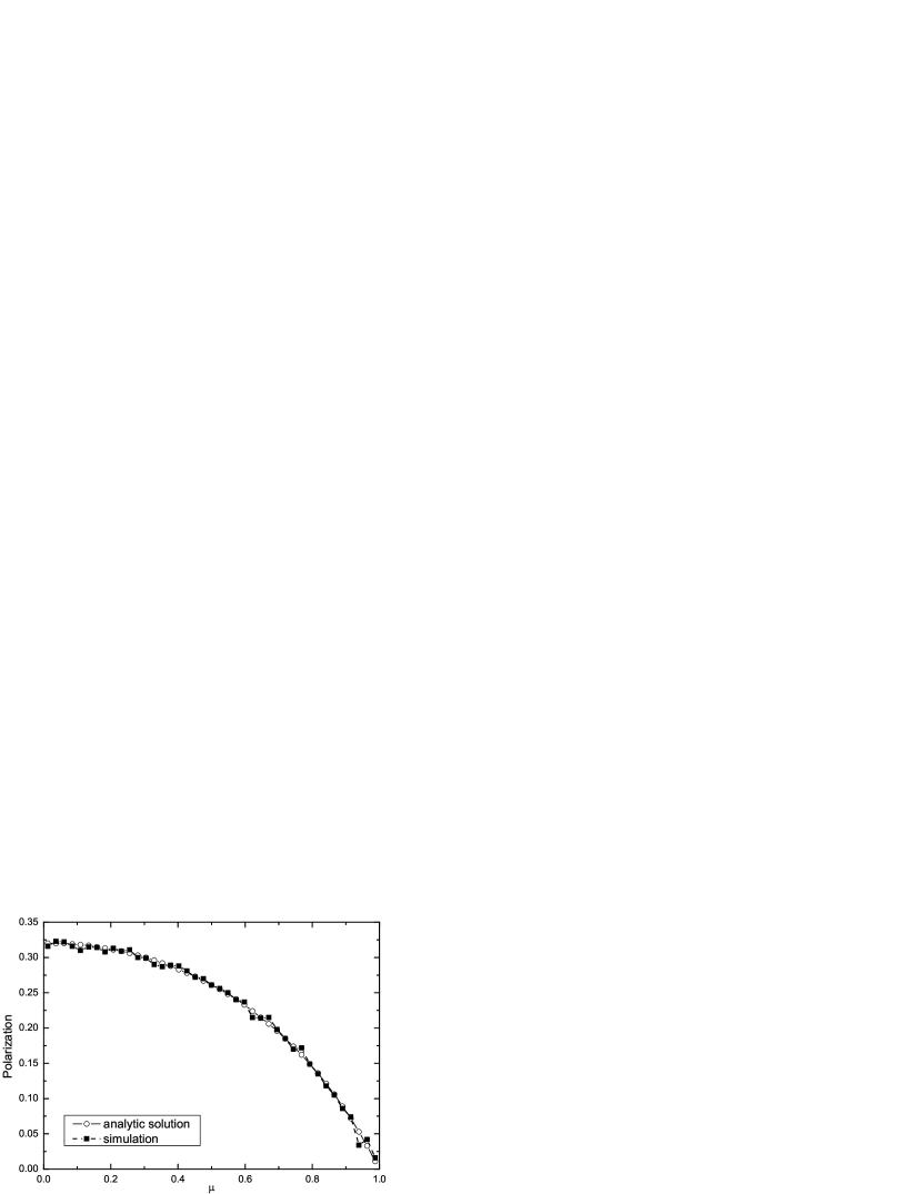
Figure 2: The output polarization of the single-scattered light viewed at different inclination angle $i$ in the case of optically thin limit ($\tau<<1$). The geometry of the scatterer is presented in Fig. 1. Here $\mu=\cos i$, $\theta_{0}=12^{\rm o}$, and $N_{e}$ = $4\times 10^{23}$ cm^-2. The analytic result is presented as open circles (eq. 7), and the simulation resuls as black squares.

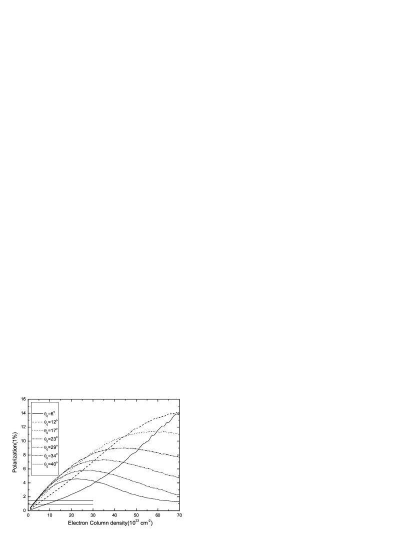
Figure 3: The average continuum polarization degree for BAL QSO as a function of the column density for different $\theta_{0}$, based on Monte-Carlo simulations. The two horizontal lines mark the polarization degree 0.93% (the average value of HiBAL QSOs) and 1.46% (the average of LiBAL QSOs). The data

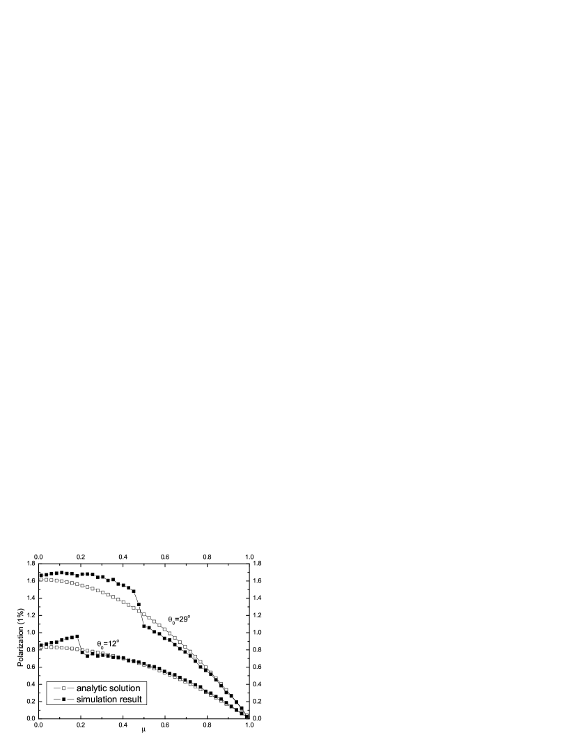
Figure 4: The effect of the radiation transfer on the output polarization for $N_{e}=4\times 10^{23}$ cm^-2 ($\tau_{e}=0.266$). The analytic result takes into account of only single scattering while both multiple scattering and the attenuation of the direct light is considered in the Monte-Carlo simulation.

Following the procedures described in §2, we perform Monte-Carlo simulations to correct the effect of radiative transfer. We test the Monte-Carlo code by simulating single scattering process, and found the results from the simulations are in good agreement with the analytic ones (Fig. 2). In the simulations below, we consider the half covering angle $\theta_{0}$ from 6^o to 40^o and the column density of electron $N_{e}$ from $10^{23}$ cm^-2 to $7\times 10^{24}$ cm^-2. In Fig. 3 we plot the resulted average continuum polarization degree ($\bar{P}_{B}$) for BAL QSO as a function of the column density. We can see that, to produce the observed average polarization degrees of HiBAL (0.93%), the minimum column density of 2 $\times 10^{23}$ cm^-2 is required for the range of $\theta_{0}$ considered. This number increases to 3.5 $\times 10^{23}$ cm^-2 for LiBAL. Using the average $\theta_{0}=12^{\rm o}$ (corresponding to $\mu_{0}$=0.2), we derive a column density of 4 $\times 10^{23}$ cm^-2 for HiBAL, slightly higher than the analytical result. In Fig. 4, we plot the output polarization degree as a function of the viewing angle from Monte Carlo simulations, assuming $N_{e}$ = 4 $\times 10^{23}$ cm^-2 ($\tau_{e}$ = 0.266). For comparison, the analytic results, which is valid when $\tau_{e}$ $<<$ 1, are also presented. The impact of the radiative transfer to the polarization degree is apparent in the figure. Basically, because of the attenuation of the direct continuum, the radiative thransfer causes larger polariztion for BAL QSOs than that from the analytic calculation. For non-BAL QSOs, the situation is more complex. For a model with small $\theta_{0}$ = $12^{\rm o}$, the optical depth at small inclination angle is smaller, consequently the scattered photons escape more likely along the polar direction, which results in slightly larger (smaller) polariztion at smaller (larger) inclinations. However, for a model with larger $\theta_{0}$ = $29^{\rm o}$, the attenuation of the scattered light becomes important, which reduces the polarization for non-BAL QSOs.

We point out that, in additional to the observed average polarization degrees for BAL and non-BAL QSOs, the distribution of the observed polarization of a radio quiet QSO sample can provide further constraints to the model of the scatterer. We consider the optically thin case first. For a given axisymmetric electron-scatterer, the polarization degrees at different view angles $i$ follow eq. 7. The normalized distribution of the polarization degree can thus be written as

$$\frac{dN}{dp}=\frac{1}{dp/d\mu}=\frac{1}{2p_{0}\sqrt{1-p/p_{0}}}\;\;{\mathrm{for}}\;p\leq p_{0}$$ (12)

where $p_{0}$ is the polarization degree viewed at the direction perpendicular to the symmetric axis. Note $p_{0}$ depends on the optical depth and the geometry of the scatterer. We notice that the distribution is a monotonic increasing function of $p$ for a given scatterer. Monte-Carlo simulations, which taking account of radiative transfer for larger optical depth, give similar result (see. Fig. 5). However, an opposite trend was found in the observed distributions given by Stockman et al (1984) and Berriman et al. (1990), who found the observed distribution of polarization degree of all QSOs (including BAL QSOs) decreases with increasing $p$ above 0.2%. We argue that the discrepancy might also be explained by a dispersal distribution of the properties of the shielding gas. Here considering a distribution of $p_{0}$ as $f(p_{0})$, we can write formally the distribution of $p$ as

$$\frac{dN}{dp}=\int_{p}^{1}\frac{f(p_{0})dp_{0}}{2p_{0}\sqrt{1-p/p_{0}}}$$ (13)

If the observed distribution of the polarization is known, we can solve the above equation inversely, e.g.,through Richardson-Lucy approach, to obtain the $f(p_{0})$, which in turn can be used to constrain the geometry of the scatterer. Using the polarization distribution of QSOs presented by Stockman et al (1984, see Fig. 1 in their paper), which can be described approximately with

$$\frac{dN}{dp}=\left\{\begin{array}[]{ll}16.5&(p<0.2\%)\\ 22.23\exp(-p/0.0067)&(p>0.2\%)\end{array}\right.$$

we obtain $f(p_{0})$ in Fig. 6, which rises steeply toward lower $p_{0}$ with a peak at $p_{0}\simeq 0.34\%$. This suggests that the shielding gas in a large fraction of QSOs either have smaller column density, or smaller covering factor. Note that $P$ = $0.34\%$ is much smaller than the average continuum polarization of BAL QSOs which is 0.93%. This suggests that most of the quasars have BALR with covering factor much smaller than 0.2, thus these BALR make less contribution to the observed sample of BAL QSOs because of the smaller chance to be detected. A larger sample of radio quiet quasars with accurate measurement of the continuum polarization will help give better constraints to the distribution of the BALR properties. Note the observed distribution at the small polarization end ($p<0.2\%$) was not well constrained because of the limited accuracy of the measurements, thus the resulted shape of $f(p_{0})$ has large uncertainty.

Note that the derived $f(p_{0})$ is also valid for axisymmetric scattering models, including the polar scattering models (e.g., Ogle 1997; Lamy & Hutsemékers 2004) and possible bi-conical scattering model (Elvis 2000). The reason is that the polarization produced by axisymmetric outflow is $\propto\sin^{2}i$, but independent to the outflow model (eq.7).

In passing, we point out that the average level, as well as the angle-dependence, of the polarization degree may be affected by the anisotropic emission of the continuum source, which is neglected in the above calculations. Certain levels of anisotropy are expected in optically thick accretion disk models, which usually predict stronger emission in polar directions than on the equatorial plane. In such models, the average polarization degree would be lowered in our equatorial scatterer model, and the polarization degree increases with inclination faster than in the case of isotropic continuum emission. However, we believe that the anisotropic emission would not severely affect our results for two reasons. First, BAL QSOs are at least as luminous as non-BAL QSOs . Second, we do not find anti-correlation between the polarization degree and the continuum luminosity (Moore, R. L. & Stockman, H. S. 1984), which is expected in a model with anisotropic continuum.

4 Conclusion

We show that the X-ray absorber in the BAL QSOs is capable to reproduce the observed continuum polarization for both BAL QSOs and non-BAL QSOs. However, the covering factor of the BALR in quasars is required to have a dispersal distribution, instead of a $\delta$ function. We also find that to macth the observed distribution of the continuum polarization of radio quiet quasars, the BALR in most QSOs produces much smaller maximum continuum polarization $p0$ (while viewed edge-on) with a peak at $p0$ = 0.34%, which is much smaller than the average continuum polarization of BAL QSOs, which is 0.93%. Consequently, the BAL QSOs with small $p0$ are likely to have covering factor of BALR much smaller than 0.2, thus make less contribution to the observed sample of BAL QSOs because of the smaller chance to be detected.

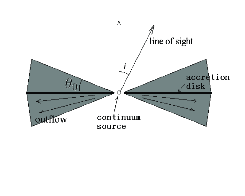
Figure 1: The geometry of the outflow model used in the paper.

Figure 5: The distributions of the polarization degree for models with $\theta_{0}=12^{\rm o}$ and $\theta_{0}=29^{\rm o}$. The left two panels are the analytic results and the two right panels are the simulation results. A column desity $N_{e}=4\times 10^{23}$ cm^-2 is assumed.

Figure 6: The reconstructed $p_{0}$ distribution assuming an axisymmetric electron-scattering model, where $p_{0}$ is the polarization degree detected on equatorial plane. See text for details.

References

- Berriman, Schmidt, West, & Stockman (1990) Berriman, G., Schmidt, G. D., West, S. C., & Stockman, H. S. 1990, ApJS, 74, 869
- Boroson (2002) Boroson, T. A. 2002, ApJ, 565, 78
- Boroson & Meyers (1992) Boroson, T. A. & Meyers, K. A. 1992, ApJ, 397, 442
- Brinkmann, Wang, Matsuoka, & Yuan (1999) Brinkmann, W., Wang, T., Matsuoka, M., & Yuan, W. 1999, A&A, 345, 43
- Canalizo & Stockton (2001) Canalizo, G. & Stockton, A. 2001, ApJ, 555, 719
- Chandrasekhar (1950) Chandrasekhar S., 1950, Radiative Transfer
- Chartas et al. (2002) Chartas, G., Brandt, W. N., Gallagher, S. C., & Garmire, G. P. 2002, ApJ, 579, 169
- Chartas et al. (2003) Chartas, G., Brandt, W. N., & Gallagher, S. C. 2003, ApJ, 595, 85
- de Kool & Begelman (1995) de Kool, M., & Begelman, M. C. 1995, ApJ, 455, 448
- Elvis (2000) Elvis, M. 2000, New Astronomy Review, 44, 559
- Elvis (2000) Elvis, M. 2000, ApJ, 545, 63
- Everett (2002) Everett J.E., 2002, submitted to ApJ
- Gallagher et al. (2000) Gallagher, S. C., Brandt, W. N., Laor, A., Elvis, M., Mathur, S., Wills, B. J., & Iyomoto, N. 2000, NASA STI/Recon Technical Report N, 91583
- Green & Mathur (1996) Green, P. J. & Mathur, S. 1996, ApJ, 462, 637
- Green et al. (2001) Green, P. J., Aldcroft, T. L., Mathur, S., Wilkes, B. J., & Elvis, M. 2001, ApJ, 558, 109
- Hamann, Korista, & Morris (1993) Hamann, F., Korista, K. T., & Morris, S. L. 1993, ApJ, 415, 541
- Hewett & Foltz (2003) Hewett, P. C., & Foltz, C. B. 2003, AJ, 125, 1784
- Hutsemkers & Lamy (2001) Hutsemkers D., Lamy H., 2001, ASP Conference Series
- Konigl & Kartje (1994) Konigl, A., & Kartje, J. F. 1994, ApJ, 434, 446
- Lamy & Hutsemékers (2004) Lamy, H., & Hutsemékers, D. 2004, A&A, 427, 107
- Lee, Blandford & Western (1994) Lee H.W., Blandford R.D., Western L., 1994, MNRAS267, 303-311
- Lee (1994) Lee H.W., 1994, MNRAS268,49-60
- Lee & Blandford (1997) Lee H.W., Blandford R.D., 1997,MNRAS, 288,19-42
- Lewis, Chapman, & Kuncic (2003) Lewis, G. F., Chapman, S. C., & Kuncic, Z. 2003, ApJ, 596, L35
- Mathur et al. (2000) Mathur S., Green P.J., Arav N., Brotherton M., Crenshaw M., Dekool M., Elvis M., Goodrich R.W., Hamann F., Hines D.C., Kashyap V., Korista K., Peterson B.M., Shields J., Shlosman I., van Breugel W., Voit M., 2000, ApJL, 533, L79-L82
- McLean & Brown (1978) McLean, I. S., & Brown, J. C. 1978, A&A, 69, 291
- Morris (1988) Morris, S. L. 1988, ApJ, 330, L83
- Moore & Stockman (1984) Moore, R. L., & Stockman, H. S. 1984, ApJ, 279, 465
- Murray et al. (1995) Murry N., Chiang J. Grossman S.A., Voit G.M., 1995, ApJ, 451, 498-509
- Ogle (1997) Ogle, P. M. 1997, ASP Conf. Ser. 128: Mass Ejection from Active Galactic Nuclei, 78
- Ogle et al. (1999) Ogle P.M., Cohen M.H., Miller J.S., Tran H.D., Goodrich R.M., Martel A.R., 1999, ApJS. 125, 1-34
- Proga, Stone, & Kallman (2001) Proga, D., Stone, J. M., & Kallman, T. R. 2001, Advances in Space Research, 28, 459
- Reichard et al. (2003) Reichard, T. A., et al. 2003, AJ, 126, 2594
- Schmidt & Hines (1999) Schmidt, G. D. & Hines, D. C. 1999, ApJ, 512, 125
- Scoville & Norman (1995) Scoville, N., & Norman, C. 1995, ApJ, 451, 510
- Stockman, Moore, & Angel (1984) Stockman, H. S., Moore, R. L., & Angel, J. R. P. 1984, ApJ, 279, 485
- Voit, Weymann, & Korista (1993) Voit, G. M., Weymann, R. J., & Korista, K. T. 1993, ApJ, 413, 95
- (38) Wang T.G., Wang J.X., Brinkmann W., Matsuoka M., 1999, ApJL. 519, L35-L38
- Weymann et al. (1991) Weymann R.J., Morris S.L., Foltz C.C., Hewett P.C., 1991, ApJ, 373, 23
- Willott, Rawlings, & Grimes (2003) Willott, C. J., Rawlings, S., & Grimes, J. A. 2003, ApJ, 598, 909