Transit Photometry of the Core-Dominated Planet HD 149026b

Abstract

We report $g$, $V$, and $r$ photometric time series of HD 149026 spanning predicted times of transit of the Saturn-mass planetary companion, which was recently discovered by Sato and collaborators. We present a joint analysis of our observations and the previously reported photometry and radial velocities of the central star. We refine the estimate of the transit ephemeris to $T_{c}~{}[{\rm HJD}]=(2453527.87455^{+0.00085}_{-0.00091})+(2.87598^{+0.00012}_{-0.00017})\ N$. Assuming that the star has a radius of $1.45\pm 0.10~{}R_{\odot}$ and a mass of $1.30\pm 0.10~{}M_{\odot}$, we estimate the planet radius to be $0.726\pm 0.064\ R_{\rm Jup}$, which implies a mean density of $1.07^{+0.42}_{-0.30}\ {\rm g\,cm^{-3}}$. This density is significantly greater than that predicted for models which include the effects of stellar insolation and for which the planet has only a small core of solid material. Thus we confirm that this planet likely contains a large core, and that the ratio of core mass to total planet mass is more akin to that of Uranus and Neptune than that of either Jupiter or Saturn.

1 Introduction

Sato et al. (2005) recently presented the discovery of a planetary companion to the bright G0 iv star HD 149026. The star exhibits a time-variable Doppler shift that is consistent with a sinusoid of amplitude $K=43$ m s^-1 and period $P=2.9$ days, which would be produced by the gravitational force from an orbiting planet with $M_{\rm P}\sin i=0.36$ $M_{\rm Jup}$. Furthermore, at the predicted time of planet-star conjunction, the star’s flux declines by 0.3% in the manner expected of an eclipse by a planet of radius $0.72$ $R_{\rm Jup}$ (given an estimate of the stellar radius, 1.45 $R_{\odot}$, that is based on the stellar parallax and effective temperature). Sato et al. (2005) observed three such eclipses. This discovery is extraordinary for at least two reasons.

Firstly, the occurrence of eclipses admits this system into the elite club of bright stars with detectable planetary transits. Of all the previously-known transiting systems, only HD 209458 (Charbonneau et al. 2000; Henry et al. 2000) and TrES-1 (Alonso et al. 2004; Sozzetti et al. 2005) have parent stars brighter than $V=12$, and therefore only they are amenable to a number of fascinating measurements requiring a very high signal-to-noise ratio. Among these studies are (i) the search for satellites and rings (Brown et al. 2001), (ii) the search for period variations due to additional companions (Wittenmyer et al. 2005), (iii) the detection of (or upper limits on) atmospheric absorption features in transmission (Charbonneau et al. 2002; Brown, Libbrecht, & Charbonneau 2002; Deming et al. 2005a), (iv) the characterization of the exosphere (Bundy & Marcy 2000; Moutou et al. 2001, 2003; Vidal-Madjar et al. 2003, 2004; Winn et al. 2004; Narita et al. 2005), (v) the measurement of the angle between the sky-projected orbit normal and stellar rotation axis (Queloz et al. 2000; Winn et al. 2005), and (vi) the search for spectroscopic features near the times of secondary eclipse (Richardson et al. 2003a, 2003b), and (vii) the direct detection of thermal emission from the planet (Charbonneau et al. 2005; Deming et al. 2005b). Charbonneau (2004) reviews these techniques and related investigations.

Secondly, the planet is the smallest and least massive of the 8 known transiting extrasolar planets. This makes HD 149026b an important test case for theories of planetary structure. Sato et al. (2005) argued that, once the effects of stellar insolation are included, the small planetary radius implies that the planet has a large and dense core. In particular, assuming a core density $\rho_{c}=5.5\ {\rm g\,cm^{-3}}$, their models predict a prodigious core mass of 78 Earth masses, or 74% of the total mass of the planet. This, in turn, would seemingly prove that the planet formed through core accretion, as opposed to direct collapse through a gravitational instability.

A system of such importance should be independently confirmed, and the determination of its basic parameters should be refined through multiple observations. With this as motivation, we performed photometry of HD 149026 on two different nights when transits were predicted by Sato et al. (2005). These observations and the data reduction procedures are described in § 2. The model that we used to determine the system parameters is described in § 3, and the results are discussed in § 4. Our data are available in digital form in the electronic version of this article, and from the authors upon request.

2 The Observations and Data Reduction

2.1 FLWO 1.2m $g$ and $r$ Photometry

We observed HD 149026 ($V=8.16$, $B-V=0.56$) on UT 2005 June 6 and UT 2005 July 2 with the 48-inch (1.2m) telescope of the F. L. Whipple Observatory (FLWO) located at Mount Hopkins, Arizona. We used Minicam, an optical CCD imager with two $2048\times 4608$ chips. In order to increase the duty cycle of the observations, we employed $2\times 2$ binning, which reduced the readout and overhead time to 20 s. Each binned pixel subtends approximately $0\farcs 6$ on the sky, giving an effective field of view of about $10\arcmin\times 23\arcmin$ for each CCD. Fortunately, there exists a nearby object of similar brightness and color (HD 149083; $V=8.05$, $B-V=0.40$, $\Delta\alpha$ $=5.1\arcmin$, $\Delta\delta=-17\arcmin$), which we employed as an extinction calibrator. We selected the telescope pointing so that both stars were imaged simultaneously. We defocused the telescope so that the full-width at half-maximum (FWHM) of a stellar image was typically 15 binned pixels (9$\arcsec$), and we used automatic guiding to ensure that the centroid of the stellar images drifted no more than 3 binned pixels over the course of the night. In addition to enabling longer integration times, this served to mitigate the effects of pixel-to-pixel sensitivity variations that were not perfectly corrected by our flat-fielding procedure. On UT 2005 June 6, we gathered 5.5 hrs of SDSS $g$-band observations with typical integration times of 8 s and a cadence of 28 s. The conditions were photometric, and the frames span an airmass from 1.01 to 1.74. On UT 2005 July 2, we gathered 4.4 hrs of SDSS $r$-band observations with integration times of 6 s and a median cadence of 26 s. The field appeared to remain free of clouds for the duration of the observations, which spanned an airmass range of 1.01 to 1.43, although occasional patches of high cirrus could be seen in images from the MMT all-sky camera.

We converted the image time stamps to Heliocentric Julian Day (HJD) at mid-exposure. The images were overscan-subtracted, trimmed, and divided by a flat-field image. We performed aperture photometry of HD 149026 and the comparison star HD 149083, using an aperture radius of 15 binned pixels (9$\arcsec$) for the UT 2005 June 6 data, and an aperture radius of 20 binned pixels (12$\arcsec$) for the UT 2005 July 2 data. We subtracted the underlying contribution from the sky for both the target and calibrator by estimating the counts in an annulus exterior to the photometric aperture. The relative flux of HD 149026 was computed as the ratio of the fluxes within the two apertures. Normalization and residual extinction corrections are described in § 3.

2.2 TopHAT $V$ Photometry at FLWO

TopHAT is an automated telescope located on Mt. Hopkins, Arizona, which was designed to perform multi-color photometric follow-up of transiting extrasolar planet candidates identified by the HAT network (Bakos et al. 2004). Since TopHAT has not previously been described in the literature, we digress briefly to outline the principal goals and features of the instrument.

Wide-field transit surveys must contend with a large rate of astrophysical false positives, which result from stellar systems that contain an eclipsing binary and precisely mimic the single-color photometric light curve of a Jupiter-sized planet transiting a Sun-like star (Brown 2003; Charbonneau et al. 2004; Mandushev et al. 2005; Torres et al. 2004). Although multi-epoch radial velocity follow-up is an effective tool for identifying these false positives (e.g. Latham 2003), instruments such as TopHAT and Sherlock (Kotredes et al. 2004) can be fully-automated, and thus offer a very efficient means of culling the bulk of such false positives. TopHAT is a 0.26m diameter f/5 commercially-available Baker Ritchey-Chrétien telescope on an equatorial fork mount developed by Fornax Inc. A 1$\fdg$25-square field of view is imaged onto a 2k$\times$2k Peltier-cooled, thinned CCD detector, yielding a pixel scale of 2$\farcs$2. The time for image readout and associated overheads is 25 s. Well-focused images have a typical FWHM of 2 pixels. A two-slot filter-exchanger permits imaging in either $V$ or $I$. The components are protected from inclement weather by an automated asymmetric clamshell dome.

We observed HD 149026 on UT 2005 July 2, the same night as the FLWO 1.2m $r$ observations described above. In order to extend the integration times and increase the duty cycle of the observations, we broadened the point spread function (PSF) by performing small, regular motions in RA and DEC according to a prescribed pattern that was repeated during each 13 s integration (see Bakos et al. 2004 for details). The resulting PSF had a FWHM of 3.5 pixels (7$\farcs$7). We gathered 4.8 hrs of $V$ observations with a cadence of 68 s, spanning an airmass range of 1.01 to 1.45.

We converted the time stamps in the image headers to HJD at mid-exposure. We calibrated the images by subtracting the overscan bias and a scaled dark image, and dividing by an average sky flat from which large outliers had been rejected. We evaluated the centroids of the target and the three brightest calibrators in each image. For each star, we summed the flux within an aperture with a radius of 8 pixels (17$\farcs$6), and subtracted a local sky estimate based on the median flux in an annulus exterior to the photometric aperture. We divided the resulting time series for the target by the statistically-weighted average of the time series for the three calibrator stars. The resulting relative flux time series was then corrected for normalization and residual extinction effects as described in the following section.

3 The Model

We attempted to fit simultaneously (i) the 3 photometric time series discussed above, (ii) the $(b+y)/2$ photometry of 3 transits presented by Sato et al. (2005), and (iii) the 7 radial velocities that were measured by Sato et al. (2005) when the planet was not transiting. We did not attempt to fit the 4 radial velocities measured during transits, which would have required a model of the Rossiter-McLaughlin effect (Queloz et al. 2002; Ohta, Taruya, & Suto 2004; Winn et al. 2005).

We modeled the system as a circular Keplerian orbit. Following Sato et al. (2005), we assumed the stellar mass ($M_{\rm S}$) to be $1.30~{}M_{\odot}$ and the stellar radius ($R_{\rm S}$) to be $1.45~{}R_{\odot}$. The free parameters were the planetary mass ($M_{\rm P}$), planetary radius ($R_{\rm P}$), orbital inclination ($i$), orbital period ($P$), central transit time ($T_{c}$), and the heliocentric radial velocity of the center of mass ($\gamma$). We included 2 free parameters for each of our 3 photometric time series: an overall flux scaling $C$; and a residual extinction coefficient ($k$) to correct for differential extinction between the target star and the comparison object, which have somewhat different colors. These are defined such that the relative flux observed through an airmass $X$ is $C\exp(-kX)$ times the true relative flux. The residual extinction corrections were small but important at the millimagnitude level; for example, in the $g$ band, we found $k\approx-2\times 10^{-3}$. The 3 time series presented by Sato et al. (2005) were already corrected for airmass, so we allowed each of these to have only an independent flux scaling. Finally, we allowed the data from each spectrograph (Keck/HIRES and Subaru/HDS) to have an independent value of $\gamma$.

We computed the model radial velocity at each observed time as $\gamma+\Delta v_{r}$, where $\Delta v_{r}$ is the line-of-sight projection of the orbital velocity of the star. We calculated the model flux during transit using the linear limb-darkening law $B_{\lambda}(\mu)=1-u_{\lambda}(1-\mu)$, where $B_{\lambda}$ is the normalized stellar surface brightness profile and $\mu$ is the cosine of the angle between the normal to the stellar surface and the line of sight. We employed the “small planet” approximation as described by Mandel & Agol (2002). We held the limb darkening parameter $u_{\lambda}$ fixed at a value appropriate for a star with the assumed properties, and for the bandpass concerned, according to the models of Claret & Hauschildt (2003) and Claret (2004). These values were $u_{g}=0.73$, $u_{r}=0.61$, $u_{V}=0.62$, and $u_{b+y}=0.67$.

The goodness-of-fit parameter is

$$\chi^{2}=\chi^{2}_{v}+\chi^{2}_{f}=\sum_{n=1}^{N_{v}}\left(\frac{v_{O}-v_{C}}{\sigma_{v}}\right)^{2}+\sum_{n=1}^{N_{f}}\left(\frac{f_{O}-f_{C}}{\sigma_{f}}\right)^{2},$$ (1)

where $v_{O}$ and $v_{C}$ are the observed and calculated radial velocities, of which there are $N_{v}=7$, and $f_{O}$ and $f_{C}$ are the observed and calculated fluxes, of which there are $N_{f}=2310$. Of the flux measurements, 679 are our $g$-band measurements, 574 are our $r$-band measurements, 237 are our $V$-band measurements, and 820 are the $(b+y)$/2 measurements of Sato et al. (2005). We minimized $\chi^{2}$ using an AMOEBA algorithm (Press et al. 1992).

The radial velocity uncertainties $\sigma_{v}$ were taken from Table 2 of Sato et al. (2005). To estimate the uncertainties in our photometry, we performed the following procedure. We expect the two dominant sources of uncertainty to be scintillation noise ($\sigma_{S}$) and Poisson noise ($\sigma_{P}$). Young (1967) advocated an approximate scaling law for the fractional error due to scintillation noise (see also Dravins et al. 1998):

$$\sigma_{S}=0.06\ X^{7/4}\left(\frac{D}{{\rm 1~{}cm}}\right)^{-2/3}\left(\frac{t_{\rm exp}}{{\rm 1~{}s}}\right)^{-1/2}\exp\left(-\frac{h}{{\rm 8000~{}m}}\right),$$ (2)

where $X$ is the airmass, $D$ is the diameter of the aperture, $t_{\rm exp}$ is the exposure time, and $h$ is the altitude of the observatory. For each of our 3 time series, we assumed that the noise in each point obeyed

$$\sigma=\sqrt{\sigma_{P}^{2}+(\beta\sigma_{S})^{2}},$$ (3)

where $\sigma_{S}$ was calculated with Eq. 2. We determined the constant $\beta$ by requiring $\chi^{2}/N_{\rm DOF}=1$ for that particular time series. Thus we did not attempt to use the $\chi^{2}$ statistic to test the validity of the model; rather, we assumed the model is correct, and sought the appropriate weight for each data point. The results for $\beta$ ranged from 1.2 to 1.5. To estimate the uncertainties in each of the three Sato et al. (2005) time series (which were already corrected for airmass), we simply assigned an airmass-independent error bar to all the points such that $\chi^{2}/N_{\rm DOF}=1$. The results agreed well with the RMS values quoted in Table 5 of Sato et al. (2005).

After assigning the weight of each data point in this manner, we analyzed all the data simultaneously and found the best-fitting solution. This solution is overplotted on the data in Figure 1. Our photometry, after correcting for the overall flux scale and for airmass, is given in Table 1. We estimated the uncertainties in the model parameters using a Monte Carlo algorithm, in which the optimization was performed on each of $7\times 10^{4}$ synthetic data sets, and the distribution of best-fitting values was taken to be the joint probability distribution of the parameters. Each synthetic data set was created as follows:

1. We randomly drew $N_{f}=2310$ flux measurements $\{t_{n},f_{n}\}$ from the real data set. We drew these points with replacement, i.e., we allowed for repetitions of the original data points. This procedure, recommended by Press et al. (1992), estimates the probability distribution of the measurements using the measured data values themselves, rather than the more traditional approach of assuming a certain model for the underlying process.

2. This procedure was impractical for the radial velocity measurements, because the number of data points is too small. Instead, in each realization, we discarded a single radial velocity measurement chosen at random. This was intended as a test of the robustness of the results to single outliers. To each of the remaining $N_{v}=6$ radial velocities, we added a random number drawn from a Gaussian distribution, with zero mean and a standard deviation equal to the quoted 1 $\sigma$ uncertainty.

3. To account for the uncertainty in the stellar properties, we assigned a stellar mass by picking a random number from a Gaussian distribution with mean $1.30~{}M_{\odot}$ and standard deviation $0.10~{}M_{\odot}$. Likewise, for the stellar radius, we used a Gaussian distribution with a mean of $1.45~{}R_{\odot}$ and a standard deviation of $0.10~{}R_{\odot}$. We note that this procedure does not take into account the intrinsic correlation between these two variables that is expected from models of stellar structure and evolution. Assuming a stellar mass-radius relation would provide an independent constraint that would reduce the overall uncertainty on the planetary radius (Cody & Sasselov 2002). We elected not to make such an assumption because the stellar age, and therefore its evolutionary state, are not known with sufficient precision.

4 Discussion and Conclusions

Figure 1: Radial velocity variations and photometry of HD 149026. The upper two panels show the radial velocity measurements by Sato et al. (2005), as a function of time (left) and orbital phase (right). Open symbols are Subaru/HDS measurements, and filled circles are Keck/HIRES measurements. The best-fitting value of $\gamma$ (for each spectrograph) has been subtracted from the data. The best-fitting model is overplotted. The remaining panels show the photometry from this work and Sato et al. (2005). Although the points have been averaged into 5 minute bins for presentation purposes (10 minute bins, for TopHAT), the fitting procedure was performed on unbinned data.

The best-fitting model is illustrated in Fig. 1. The estimated probability distribution for each model parameter is shown in Fig. 2. Some of the parameters have correlated uncertainties, as shown in Fig. 3. In addition to showing correlations among the model parameters, Fig. 3 shows the distributions for three fundamental properties of a single-transit light curve: the transit depth in the absence of stellar limb-darkening, defined as $(R_{\rm P}/R_{\rm S})^{2}$; the transit duration, defined as the time between first and fourth contact ($t_{\rm IV}-t_{\rm I}$); and the ingress duration, defined as the time between first and second contact ($t_{\rm II}-t_{\rm I}$). Since we have assumed a circular Keplerian orbit, the ingress and egress durations are equal. The contact times can be calculated from our model parameters via the relations

$$\sin i\hskip 1.4457pt\cos\frac{\pi(t_{\rm IV}-t_{\rm I})}{P} = \sqrt{1-\left(\frac{R_{\rm S}+R_{\rm P}}{a}\right)^{2}}$$

$$\sin i\hskip 1.4457pt\cos\frac{\pi(t_{\rm II}-t_{\rm I})}{P} = \sqrt{1-\left(\frac{R_{\rm S}-R_{\rm P}}{a}\right)^{2}},$$ (4)

where $a$ is the semi-major axis, given by Kepler’s law $G(M_{\rm S}+M_{\rm P})/a^{3}=(2\pi/P)^{2}$.

Figure 2: Estimated probability distributions of some planetary, stellar, and orbital parameters. The dotted histograms show the results of fits to all $7\times 10^{4}$ Monte Carlo realizations of the data. The solid histograms show the results for the cases when the biggest radial velocity outlier is dropped; we favor these results for reasons described in the text. The one-dimensional probability distribution for $i$ (lower left panel) shows a secondary peak near $i=90\arcdeg$, which contains 9% of the solutions. We clip these solutions prior to determining the best-fit values and confidence limits (see text). Solid vertical lines show the median value of each of the solid histograms. Dashed vertical lines show the 68.3% confidence limits.

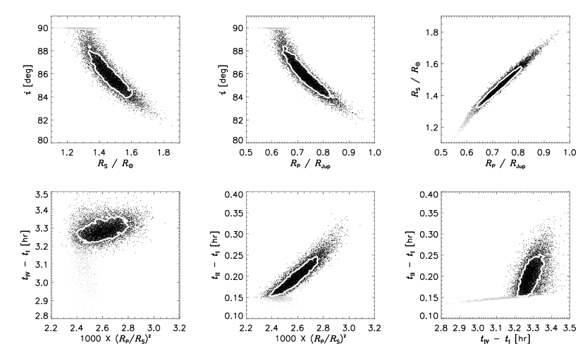
Figure 3: Joint probability distributions of some planetary, stellar, and orbital parameters, based on the $10^{4}$ Monte Carlo realizations in which $v_{3}$ was dropped. The density of points is proportional to the probability density. The white contours are isoprobability contours enclosing 68.3% of the points. Solutions with $i>89\fdg 75$ (an arbitrary threshold) are colored gray to distinguish between the two solution branches described in the text.

We found that the probability distributions did not depend significantly on which of the 7 radial velocity measurements were discarded, with the important exception of the third Subaru/HDS measurement ($v_{3}=-42.48\pm 3.10$ m s^-1 at HJD 2453208.909939). When this point was dropped, the results for the orbital period, planetary mass, and velocity offsets changed by 1 $\sigma$. In Fig. 2, the solid histograms show the results of the $10^{4}$ trials for which $v_{3}$ was discarded, and the dotted histograms show the results of all $7\times 10^{4}$ trials. We believe that either the model fails to accurately describe $v_{3}$ within its quoted uncertainty (due to a missing ingredient such as a nonzero eccentricity or an additional planetary companion), or that the true uncertainty in this measurement is larger than the estimate (due to stellar jitter or some other source of systematic error). In support of this claim, we note that this single point makes a disproportionate contribution to $\chi^{2}_{v}$. When any single radial velocity measurement besides $v_{3}$ is dropped, the minimum $\chi^{2}_{v}$ ranges from 13 to 19. Yet when $v_{3}$ is dropped, $\chi^{2}_{v}=0.5$. In Table 2, we present the results for the cases in which $v_{3}$ is dropped. Our intention is to avoid biased results from an oversimplified model or an underestimated uncertainty.

The one-dimensional probability distribution for $i$ shows that the majority of solutions favor $i\approx 86\arcdeg$, but a peak is evident at $i=90\arcdeg$ (see the lower left panel of Fig. 2). We identify these maximum-$i$ solutions by applying an arbitrary cut-off of $i>89\fdg 75$, and we display these solutions with a distinct coloring in Fig. 3. These solutions, which account for 9% of the total, represent a pile-up at equatorial configurations owing to the numerical constraint $i\leq 90\arcdeg$. We exclude this solution subset prior to determining the best-fit values and confidence limits listed in Table 2. We note that the duration of ingress and egress is significantly shorter for HD 149026 than for either HD 209458 or TrES-1. The available photometry samples the times of ingress and egress only sparsely. We encourage high-cadence monitoring of these key portions of the transit curve.

Based on this analysis, our best estimate of the transit ephemeris is

$$T_{c}~{}[{\rm HJD}]=(2453527.87455^{+0.00085}_{-0.00091})+(2.87598^{+0.00012}_{-0.00017})\ N.$$ (5)

Tabulation of the observed time of each eclipse is of interest because deviations from the predictions of a single-period ephemeris could indicate the presence of planetary satellites or additional planetary companions (Brown et al. 2001, Miralda-Escudé 2002). In particular, terrestrial planets that induce a radial-velocity perturbation below current detection limits can nonetheless be detected through accurate eclipse timing (Holman & Murray 2005, Agol et al. 2005). We searched for evidence of timing anomalies as follows. We constructed a model transit light curve for each of the 4 bandpasses [$g$, $r$, $V$, and $(b+y)/2$], based on the optimal parameters appearing in Table 2 and the appropriate limb darkening coefficient (§ 3). For each of the 6 extinction-corrected, normalized light curves (identified by an index $j$), we then evaluated the $\chi^{2}$ of the fit as a function of assumed time of center of eclipse, $T_{c}^{j}$. After we identified the optimal value for $T_{c}^{j}$, we assigned uncertainties by identifying the timing offsets at which the value of $\chi^{2}$ had increased by 1. We list these values in Table 3, and plot the “observed minus calculated” ($O-C$) residuals in Figure 4. The typical timing precision is 2 minutes, which is comparable to results from other ground-based photometry (for a tabulation of $O-C$ for other transiting-planet systems, see Charbonneau et al. 2005 for TrES-1, and Wittenmyer et al. 2005 for HD 209458). We find no evidence for deviations from the predictions of a constant orbital period. We encourage future monitoring of the times of eclipse of this system. In particular, space-based observations (Brown et al. 2001) should achieve a substantial improvement in timing precision, and thus permit a more sensitive search for perturbing planets.

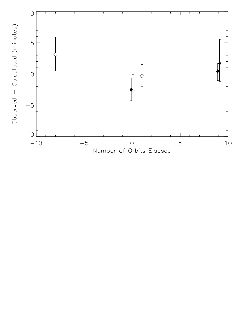
Figure 4: The “observed minus calculated” ($O-C$) residuals for the 3 light curves presented in this paper (black diamonds) and for the 3 light curves in Sato et al. (2005, open diamonds). In the two cases where two estimates are available for the same transit, we have slightly offset the values along the horizontal axis for clarity. The assumed ephemeris is given in Eq. 5. The data plotted here are given in Table 3.

Due to its favorable apparent brightness, the HD 149026 system will be particularly amenable to a variety of follow-up studies. Such pursuits will be more observationally challenging than was the case for HD 209458, owing to the smaller size of the planet relative to the parent star. Nonetheless, we are certain that such challenges will be met and overcome. Now that a handful of transiting planets of bright stars have been identified, the long-sought-after goal of comparative exoplanetology may be realized.

Table 1: Photometry of HD 149026

Telescope	Filter	HJD	Relative flux	Uncertainty
FLWO48	g	$2453527.750311$	$0.9983$	$0.0018$
FLWO48	g	$2453527.750624$	$0.9984$	$0.0018$
FLWO48	g	$2453527.750936$	$0.9988$	$0.0018$
FLWO48	g	$2453527.751260$	$0.9999$	$0.0018$
FLWO48	g	$2453527.751585$	$1.0006$	$0.0018$

Note. — The quoted uncertainties are based on the procedure described in § 2, which assumes that our model is correct. We intend for this Table to appear in entirety in the electronic version of the Astronomical Journal. A portion is shown here to illustrate its format. The data are also available in digital from the authors upon request.

Table 2: System Parameters of HD 149026

Parameter	Best fit	68% conf. limits
		lower	upper
$M_{\rm S}$ [$M_{\odot}$]	$1.30$	$-0.10$	$+0.10$
$R_{\rm S}$ [$R_{\odot}$]	$1.45$	$-0.10$	$+0.10$
$M_{\rm P}$ [$M_{\rm Jup}$]	$0.330$	$-0.023$	$+0.022$
$R_{\rm P}$ [$R_{\rm Jup}$]	$0.726$	$-0.062$	$+0.066$
$P$ [days]	$2.87598$	$-0.00017$	$+0.00012$
$T_{c}-2453527$ [HJD]	$0.87455$	$-0.00091$	$+0.00085$
$i$ [deg]	$85.8$	$-1.3$	$+1.6$
$\gamma_{\rm HIRES}$ [m s-1]	$6.6$	$-1.8$	$+1.8$
$\gamma_{\rm HIRES}-\gamma_{\rm HDS}$ [m s-1]	$5.8$	$-2.8$	$+2.6$

Note. — Results are based on fits to the $10^{4}$ Monte Carlo realizations of the data in which $v_{3}$ was dropped (see § 3). Values for $M_{\rm S}/M_{\odot}$ were drawn from a Gaussian random distribution with mean 1.30 and standard deviation 0.1. Values for $R_{\rm S}/R_{\odot}$ were drawn from a Gaussian random distribution with mean 1.45 and standard deviation 0.1. All other quantities listed in this table were free parameters in the model.

Table 3: Observed Times of Transit

Event	$T_{c}\ [{\rm HJD}]$	$N_{\rm elapsed}$	$\sigma_{\rm HJD}$	$(O-C)$	$\frac{(O-C)}{\sigma_{\rm HJD}}$
Sato et al. (2005)	2453504.8689	$-$8.0	0.0019	$+$0.0022	$+$1.15
Sato et al. (2005)	2453527.8727	0.0	0.0017	$-$0.0018	$-$1.09
This work [FLWO48 $g$]	2453527.8728	0.0	0.0012	$-$0.0018	$-$1.41
Sato et al. (2005)	2453530.7503	$+$1.0	0.0012	$-$0.0002	$-$0.17
This work [FLWO48 $r$]	2453553.7587	$+$9.0	0.0010	$+$0.0003	$+$0.32
This work [TopHAT $V$]	2453553.7597	$+$9.0	0.0023	$+$0.0012	$+$0.51

References

- Agol et al. (2005) Agol, E., Steffen, J., Sari, R., & Clarkson, W. 2005, MNRAS, 359, 567
- Alonso et al. (2004) Alonso, R., et al. 2004, ApJ, 613, L153
- Bakos et al. (2004) Bakos, G., Noyes, R. W., Kovács, G., Stanek, K. Z., Sasselov, D. D., & Domsa, I. 2004, PASP, 116, 266
- Bouchy et al. (2004) Bouchy, F., Pont, F., Santos, N. C., Melo, C., Mayor, M., Queloz, D., & Udry, S. 2004, A&A, 421, L13
- Brown (2003) Brown, T. M. 2003, ApJ, 593, L125
- Brown, Libbrecht, & Charbonneau (2002) Brown, T. M., Libbrecht, K. G., & Charbonneau, D. 2002, PASP, 114, 826
- Brown et al. (2001) Brown, T. M., Charbonneau, D., Gilliland, R. L., Noyes, R. W., & Burrows, A. 2001, ApJ, 552, 699
- Bundy & Marcy (2000) Bundy, K. A., & Marcy, G. W. 2000, PASP, 112, 1421
- Charbonneau et al. (2000) Charbonneau, D., Brown, T. M., Latham, D. W., & Mayor, M. 2000, ApJ, 529, L45
- Charbonneau et al. (2002) Charbonneau, D., Brown, T. M., Noyes, R. W., & Gilliland, R. L. 2002, ApJ, 568, 377
- Charbonneau (2004) Charbonneau, D. 2004, IAU Symposium, 219, 367
- Charbonneau et al. (2004) Charbonneau, D., Brown, T. M., Dunham, E. W., Latham, D. W., Looper, D. L., & Mandushev, G. 2004, AIP Conf. Proc. 713: The Search for Other Worlds, 713, 151
- Charbonneau et al. (2005) Charbonneau, D., et al. 2005, ApJ, 626, 523
- Claret & Hauschildt (2003) Claret, A., & Hauschildt, P. H. 2003, A&A, 412, 241
- Claret (2004) Claret, A. 2004, A&A, 428, 1001
- Cody & Sasselov (2002) Cody, A. M., & Sasselov, D. D. 2002, ApJ, 569, 451
- Deming et al. (2005a) Deming, D., Brown, T. M., Charbonneau, D., Harrington, J., & Richardson, L. J. 2005a, ApJ, 622, 1149
- Deming et al. (2005b) Deming, D., Seager, S., Richardson, L. J., & Harrington, J. 2005b, Nature, 434, 740
- Dravins et al. (1998) Dravins, D., Lindegren, L., Mezey, E., & Young, A. T. 1998, PASP, 110, 610
- Henry et al. (2000) Henry, G. W., Marcy, G. W., Butler, R. P., & Vogt, S. S. 2000, ApJ, 529, L41
- Holman & Murray (2005) Holman, M. J., & Murray, N. W. 2005, Science, 307, 1288
- Holman et al. (2005) Holman, M. J., Winn, J. N., Stanek, K. Z., Torres, G., Sasselov, D. D., Allen, R. L. Fraser, W. ApJ, submitted, astro-ph/0506569
- Konacki et al. (2005) Konacki, M., Torres, G., Sasselov, D. D., & Jha, S. 2005, ApJ, 624, 372
- Konacki et al. (2003) Konacki, M., Torres, G., Jha, S., & Sasselov, D. D. 2003, Nature, 421, 507
- Kotredes et al. (2004) Kotredes, L., Charbonneau, D., Looper, D. L., & O’Donovan, F. T. 2004, AIP Conf. Proc. 713: The Search for Other Worlds, 713, 173
- Latham (2003) Latham, D. W. 2003, ASP Conf. Ser. 294: Scientific Frontiers in Research on Extrasolar Planets, 294, 409
- Mandel & Agol (2002) Mandel, K., & Agol, E. 2002, ApJ, 580, L171
- Mandushev et al. (2005) Mandushev, G., et al. 2005, ApJ, 621, 1061
- Miralda-Escudé (2002) Miralda-Escudé, J. 2002, ApJ, 564, 1019
- Moutou et al. (2001) Moutou, C., Coustenis, A., Schneider, J., St Gilles, R., Mayor, M., Queloz, D., & Kaufer, A. 2001, A&A, 371, 260
- Moutou et al. (2003) Moutou, C., Coustenis, A., Schneider, J., Queloz, D., & Mayor, M. 2003, A&A, 405, 341
- Moutou et al. (2004) Moutou, C., Pont, F., Bouchy, F., & Mayor, M. 2004, A&A, 424, L31
- Narita et al. (2005) Narita, N. et al. 2005, PASJ, in press, astro-ph/0504540
- Ohta et al. (2005) Ohta, Y., Taruya, A., & Suto, Y. 2005, ApJ, 622, 1118
- Pont et al. (2004) Pont, F., Bouchy, F., Queloz, D., Santos, N. C., Melo, C., Mayor, M., & Udry, S. 2004, A&A, 426, L15
- Press et al. (1992) Press, W. H., Teukolsky, S. A., Vetterling, W. T., & Flannery, B. P. 1992, Numerical Recipes in C (Cambridge University Press), pp. 408, 689
- Queloz et al. (2000) Queloz, D., Eggenberger, A., Mayor, M., Perrier, C., Beuzit, J. L., Naef, D., Sivan, J. P., & Udry, S. 2000, A&A, 359, L13
- Richardson et al. (2003a) Richardson, L. J., Deming, D., & Seager, S. 2003a, ApJ, 597, 581
- Richardson et al. (2003b) Richardson, L. J., Deming, D., Wiedemann, G., Goukenleuque, C., Steyert, D., Harrington, J., & Esposito, L. W. 2003b, ApJ, 584, 1053
- Sato et al. (2005) Sato, B. et al. 2005, ApJ, in press, astro-ph/0507009
- Sozzetti et al. (2004) Sozzetti, A., et al. 2004, ApJ, 616, L167
- Torres et al. (2004) Torres, G., Konacki, M., Sasselov, D. D., & Jha, S. 2004, ApJ, 614, 979
- Udalski et al. (2004) Udalski, A., Szymanski, M. K., Kubiak, M., Pietrzynski, G., Soszynski, I., Zebrun, K., Szewczyk, O., & Wyrzykowski, L. 2004, Acta Astronomica, 54, 313
- Udalski et al. (2002) Udalski, A., Szewczyk, O., Zebrun, K., Pietrzynski, G., Szymanski, M., Kubiak, M., Soszynski, I., & Wyrzykowski, L. 2002, Acta Astronomica, 52, 317
- Vidal-Madjar et al. (2003) Vidal-Madjar, A., Lecavelier des Etangs, A., Désert, J.-M., Ballester, G.E., Ferlet, R., Hébrard, G., & Mayor, M. 2003, Nature, 422, 143
- Vidal-Madjar et al. (2004) Vidal-Madjar, A., et al. 2004, ApJ, 604, L69
- Winn et al. (2005) Winn, J. N. et al. 2005, ApJ, in press, astro-ph/0504555
- Wittenmyer et al. (2005) Wittenmyer, R. A. et al. 2005, ApJ, in press, astro-ph/0504579
- Young (1967) Young, A. T. 1967, AJ, 72, 747