The XMM Large-Scale Structure Survey: An initial sample of galaxy groups and clusters to a redshift $z<0.6$

Abstract

We present X–ray and optical spectroscopic observations of twelve galaxy groups and clusters identified within the XMM Large–Scale Structure (LSS) survey. Groups and clusters are selected as extended X–ray sources from a 3.5 $\rm deg^{2}$ XMM image mosaic above a flux limit $8\times 10^{-15}\,\rm erg\,s^{-1}\,cm^{-2}$ in the [0.5–2] keV energy band. Deep $BVRI$ images and multi–object spectroscopy confirm each source as a galaxy concentration located within the redshift interval $0.29<z<0.56$. We combine line–of–sight velocity dispersions with the X–ray properties of each structure computed from a two–dimensional surface brightness model and a single temperature fit to the XMM spectral data. The resulting distribution of X–ray luminosity, temperature and velocity dispersion indicate that the XMM–LSS survey is detecting low–mass clusters and galaxy groups to redshifts $z<0.6$. Confirmed systems display little or no evidence for X–ray luminosity evolution at a given X–ray temperature compared to lower redshift X–ray group and cluster samples. A more complete understanding of these trends will be possible with the compilation of a statistically complete sample of galaxy groups and clusters anticipated within the continuing XMM–LSS survey.

1 Introduction

Surveys of distant galaxy clusters map the distribution in the universe of large amplitude density fluctuations, and so constrain key cosmological parameters and permit secondary studies to determine how X–ray gas and galaxy evolution proceeds as a function of environment. Wide area X-ray surveys are well placed to compile statistically well–defined samples of distant galaxy clusters because a) both source confusion and the X-ray background are low compared to optical searches, b) computation of the selection function and volume sampled is straightforward and c) the selection of extended X-ray emitting sources is sensitive to the signature of hot gas contained within massive, gravitationally bound structures.

A number of systematic X-ray studies have extended both the maximum redshift (i.e. the most luminous galaxy clusters) and the minimum luminosity (i.e the least massive structures) to which X–ray clusters can be identified. A comprehensive review is provided by Rosati, Borgani & Norman (2002). The principal aim of such surveys for distant, X-ray emitting clusters is to determine their space density evolution as a function of redshift and to constrain the combination of the root mean square mass density fluctuations on 8$h^{-1}$ Mpc scales, $\sigma_{8}$, and the overall matter density of the Universe expressed as fraction of the closure density, $\Omega_{\rm M}$ (e.g. Borgani et al. 2001; Schuecker et al. 2001, Allen et al. 2003). In addition to the study of global cosmological parameters, galaxy clusters provide examples of dense cosmic environments in which it is possible to study the evolution of the hot, X–ray emitting gas (e.g. Ettori et al. 2004; Lumb et al. 2004) and to determine the nature of the cluster galaxy populations and the physical processes underlying observed trends in galaxy evolution (e.g. Yee et al. 1996; Dressler et al. 1999; Andreon et al. 2004a).

Extending our current knowledge of low luminosity (i.e. low mass) X–ray clusters represents an important challenge for the present generation of X–ray surveys performed with the XMM and Chandra facilities. The local ($z<0.25$) X–ray Luminosity Function (XLF) for galaxy clusters is currently determined to X–ray luminosities $L_{X}\sim 10^{42}\ \rm erg\,s^{-1}$ in the [0.5,2] keV energy band (Henry et al. 1992; Rosati et al. 1998; Ledlow et al. 1999; Boehringer et al. 2002). However, our understanding of such systems at redshifts $0.25<z<0.8$ is largely restricted to luminosities $L_{X}\mathbin{\lower 3.0pt\hbox{$\hbox to0.0pt{\raise 5.0pt\hbox{$\char 62\relax$}\hss}\mathchar 29208\relax$}}10^{43.5}\ \rm erg\,s^{-1}$ (Henry et al. 1992; Burke et al. 1997; Rosati et al. 1998; Vikhlinin et al. 1998; Ebeling et al. 2001).

Low luminosity ($10^{42}<L_{X}/{\rm erg\,s^{-1}}<10^{43}$) X–ray clusters correspond to low mass clusters and larger galaxy groups that form a link between poorly defined “field” environments and X–ray luminous/optically–rich clusters. If, as anticipated, X–ray clusters occupying this luminosity range display X–ray temperatures $\rm T<4$ keV, they are more likely to display the effects of non–gravitational energy input into the Intra–Cluster Medium (ICM) than hotter, more massive clusters (Ponman, Cannon & Navarro 1999). Deviations of X–ray scaling relations from simple, self–similar expectations have been studied for structures displaying a relatively wide range of mass/temperature scales at $z<0.2$ (e.g. Sanderson et al. 2003). However, the study of X–ray emitting structures – selected over an extended temperature range – at $z>0.2$ will provide an important insight into the evolution of their X–ray emitting gas. Though detailed X–ray studies of galaxy clusters at $0.2<z<0.6$ are in progress (e.g. Lumb et al. 2004), few examples of X–ray emitting structures displaying temperatures $\rm T<3$ keV are currently known at such redshifts. Clearly, compilation of a sample of X–ray emitting galaxy groups and clusters to $z<0.6$ will greatly increase the range of X-ray gas temperatures over which evolutionary effects can be studied.

Low mass clusters and groups are predicted to be sites of continuing galaxy evolution at $z<1$ (e.g. Kaufmann 1996; Baugh et al. 1996). When identifying such systems, it is important to note that extended X–ray emission arises from gravitationally bound structures. This is an important difference when X–ray selected cluster samples are compared to optical/NIR selected cluster samples – whose dynamical state can only be assessed with additional velocity data. In addition, the X–ray properties of galaxy structures (luminosity and temperature) constrain the gravitational mass of the emitting structure. Extending the currently known sample of galaxy groups and low–mass clusters at $z>0.2$ via X–ray observations will provide an important group/cluster sample with consistent mass ordering. A mass ordered cluster sample will permit several detailed studies of galaxy evolution at look back times $>3-4$ Gyr to be undertaken; e.g. morphological segregation and merger–related effects (Heldson and Ponman 2003), Butcher-Oemler effects (Andreon and Ettori 1999) and the evolution of colour and luminosity functions (Andreon et al. 2004a). To date, detailed galaxy evolution studies of moderately distant $z>0.2$, X–ray selected clusters have been performed typically for only the most X–ray bright (i.e. massive) systems, e.g. $L_{X}([0.3-3.5]\rm keV)>4\times 10^{44}$ ergs s^-1 (Yee et al. 1996; Dressler 1999). Clearly an improved sample of systems covering an extended mass interval will permit a detailed investigation of galaxy evolution effects as a function of changing environment.

The X-ray Multi–Mirror (XMM) Large Scale Structure (LSS) survey (Pierre et al. 2004) is a wide area X–ray survey with the XMM facility with the primary aim to extend detailed studies of the X-ray cluster correlation function, currently determined at $z<0.2$ as part of the REFLEX survey (Schuecker et al. 2001), to a redshift of unity. However, the XMM–LSS survey features a number of secondary aims including determination of the cosmological mass function to faint X–ray luminosities, the evolution of cluster galaxy populations and the evolution of the X–ray emitting gas in clusters selected over a range of mass scales. The nominal point source flux limit of XMM–LSS is $5\times 10^{-15}\,\rm erg\,s^{-1}\,cm^{-2}$ in the [0.5–2] keV energy band. Refregier, Valtchanov and Pierre (2002) demonstrate that (assuming a reasonable distribution of cluster surface brightness profiles) the approximate flux limit for typical extended sources is $8\times 10^{-15}\,\rm erg\,s^{-1}\,cm^{-2}$ which corresponds to a X–ray luminosity $L_{X}=1.2\times 10^{43}$ ergs s^-1 for a cluster located at a redshift $z=0.6$ and $L_{X}=4.2\times 10^{43}$ ergs s^-1 for a cluster located at a redshift $z=1$ within the adopted cosmological model (see below).

The above aims are predicated upon the compilation of a large, well–defined cluster catalogue. This paper describes the first results of the XMM–LSS survey at identifying X–ray emitting clusters at $z<0.6$. The first clusters identified at $z>0.6$ are presented in Valtchanov et al. (2004). The current paper is organised as follows; Section 2 summarises the X–ray and optical imaging data and the methods employed to select candidate clusters. Section 3 describes spectroscopic observations and reductions performed for a subset of candidate clusters. Section 4 presents the determination of cluster spectroscopic properties (redshift and line–of–sight velocity dispersion). Section 5 presents the determination of confirmed cluster X–ray properties (surface brightness and temperature fitting). Section 6 presents the current conclusions for the properties of the initial $z<0.6$ sample. Throughout this paper a Friedmann–Robertson–Walker cosmological model, characterised by the present–day parameters $\Omega_{\rm M}=0.3$, $\Omega_{\Lambda}=0.7$ and $H_{0}=70$ kms^-1 Mpc^-1, is assumed. Where used, $h$ is defined as $h=H_{0}/(100$ kms^-1Mpc^-1).

2 Identifying X–ray cluster candidates

2.1 X-ray data reduction and source detection

Galaxy cluster targets presented in this paper were selected from a mosaic of overlapping XMM pointings covering a total area of approximately 3.5 $\rm deg^{2}$. This data set represents all XMM–LSS pointings received by August 2002 and includes 15 A0-1 10 ks exposures and 15 Guaranteed Time (GT) 20 ks exposures obtained as part of the XMM Medium Deep Survey (MDS).

XMM observations were reduced employing the XMM Science Analysis System (SAS) tasks emchain and epchain for the MOS and pn detectors respectively. High background periods induced by soft–proton flaring were excluded from the event lists and raw photon images as a function of energy band were created. The raw images for each detector were processed employing an iterative wavelet technique and a Poissonian noise model with a threshold of $10^{-3}$ (equivalent to $3\sigma$ for the Gaussian case) applied to select the significant wavelet coefficients (Starck & Pierre 1998). Each wavelet filtered image was exposure corrected and an image mask (including deviant pixels, detector gaps and non–exposed detector regions) was created.

Source detection was performed on the wavelet filtered X–ray images employing the SExtractor package Bertin & Arnouts (1996). The discrimination between extended (cluster) and point–like sources (mostly AGN) was achieved employing a two–constraint test based on the half–energy radius and the SExtractor stellarity index of the sources. The applied procedure is the optimum method given the XMM PSF and the Poisson nature of the signal (Valtchanov et al., 2001). The measurement of extended source properties was performed on the EPIC/pn images as they provide the greatest sensitivity. The EPIC/MOS images were used to discard possible artefacts resulting from edge effects associated with the pn CCDs.

2.2 Optical imaging

The selection of potential galaxy members within each candidate cluster was performed employing moderately deep $BVRI$ images from the CFH12k camera on the Canada France Hawaii Telescope (CFHT) obtained as part of the VIRMOS deep imaging survey (McCracken et al. 2003). Observations were processed employing the Terapix data reduction pipeline to produce an astrometric and photometric image data set. Object catalogues were produced using SExtractor. Catalogue detection thresholds as a function of photometric band are displayed in Table 1.

Table 1: Detection thresholds as a function of photometric passband for objects detected in the optical images.

Filter	Detection threshold
	(50% AB magnitude completeness
	limit for stellar sources)
$B$	26.5
$V$	26.0
$R$	26.0
$I$	25.4

2.3 Selecting candidate clusters and member galaxies

The identification of galaxy clusters over an extended redshift interval in X–ray images is limited by the ability of the XMM facility to identify extended cluster X–ray emission in a 10ks exposure. The Half–Energy Width (HEW) of a on–axis point source is approximately 15″ at 1.5 keV. However, the HEW displays marked local variations resulting from off–axis angle, vignetting and detector gaps. The on–axis HEW corresponds to a projected transverse distance of 120 kpc at a redshift $z=1$ within the assumed cosmological model. Although this HEW is sufficient to resolve the extended emission from massive galaxy clusters to $z\mathbin{\lower 3.0pt\hbox{$\hbox to0.0pt{\raise 5.0pt\hbox{$\char 62\relax$}\hss}\mathchar 29208\relax$}}1$, the effect of low central surface brightness, leading to a truncated detectable cluster extension, can lead to a cluster being erroneously identified as an unresolved object. Therefore both distant clusters and intrinsically compact clusters at all redshifts may potentially appear as only marginally resolved or unresolved sources in XMM–LSS X–ray mosaics. A quantitative assessment of the cluster X–ray selection function will form the subject of a future paper (Pacaud et al. 2005).

The XMM–LSS incorporates a number of different solutions to the problem of cluster identification, e.g. correlation of extended X–ray sources with optical galaxy structures (this paper and Valtchanov et al. 2004), investigation of the X–ray properties of optically identified structures (and vice versa; Andreon et al. 2004b) and the investigation of extended X–ray sources lacking optical counterparts together with unresolved X-ray sources associated with faint optical structures (Andreon et al. 2004b).

Analysis of the first $3.5\ \rm deg^{2}$ of the XMM–LSS survey led to the identification of 55 extended sources with fluxes greater than $8\times 10^{-15}\,\rm erg\,s^{-1}\,cm^{-2}$ which are extended according to the criteria detailed in Section 2.1. The optical imaging data corresponding to a $7\arcmin\times 7\arcmin$ field centred upon the location of each extended X–ray source was analysed for the presence of a significant galaxy structure showing a well defined, red colour sequence (Stanford et al. 1998; Kodama et al. 1998). Candidate cluster members were selected by inspection of the available $BVRI$ photometry of objects identified within the field of each extended X–ray source. Colour magnitude thresholds were applied interactively in order to enhance galaxy structures when viewed in a $VRI$ pseudo–colour image of each field with X–ray contours superposed from the wavelet–filtered X–ray image. One exception to this procedure was cluster candidate XLSS J022722.3-032141 (see Table 2); the optical data for this candidate cluster consisted of the $I$–band VLT/FORS2 pre-image obtained to define slit locations. Candidate cluster members were selected to include all galaxies up to 1.5 magnitudes fainter than the bright ($I=17.1$), central galaxy associated with the extended X–ray source.

The sample of candidate cluster members generated by the above procedures was used to design spectroscopic masks for each candidate cluster field. Two multi–slit masks were created for each candidate cluster with brighter galaxies given higher priority in the slit assignment procedure. Unused regions of each multi–slit mask were employed to sample the population of unresolved X–ray sources with bright ($R<23$) optical counterparts. Further discussion of this additional sample will appear elsewhere.

3 Spectroscopic observations

The candidate cluster sample was observed by the Las Campanas Observatory Baade telescope with the Low Dispersion Survey Spectrograph (LDSS2) during 4-5 October 2002 and the European Southern Observatory Very Large Telescope (VLT) with Focal Reducing Spectrograph (FORS2) during 9-12 October 2002. Each instrument (LDSS2 and FORS2) is a focal reducing spectrograph with both an imaging and a multi-object spectroscopy (MOS) capability. In each case, MOS observations are performed using slit masks mounted in the instrument focal plane. Details of which cluster candidate was observed with which telescope plus instrument configuration are provided in Table 2. The effective wavelength interval, pixel sampling and spectral resolution generated by each instrument combination are indicated in Table 3.

Table 2: Observing log of candidate groups and clusters.

ID	Cluster	Right Ascension	Declination	Instrument	$\rm Grism+Filter$	# of masks	Total exposure time
							per mask (seconds)
006	XLSSUJ022145.2-034614	02:21:45.22	$-03$:46:14.1	FORS2	$\rm 300V+GG435$	2	$2700+2400$
007	XLSSUJ022406.0-035511	02:24:05.95	$-03$:55:11.4	FORS2	$\rm 600RI+GG435$	2	$2400+2400$
008	XLSSUJ022520.7-034800	02:25:20.71	$-03$:48:00.0	FORS2	$\rm 600RI+GG435$	2	$1200+1200$
009	XLSSUJ022644.2-034042	02:26:44.21	$-03$:40:41.8	FORS2	$\rm 300V+GG435$	2	$1800+1800$
010	XLSSUJ022722.2-032137	02:27:22.16	$-03$:21:37.0	FORS2	$\rm 600RI+GG435$	1	$600$
012	XLSSUJ022827.5-042554	02:28:27.47	$-04$:25:54.3	LDSS2	medium-red	2	$1800+1800$
013	XLSSUJ022726.0-043213	02:27:25.98	$-04$:32:13.1	LDSS2	medium-red	2	$900+900$
014	XLSSUJ022633.9-040348	02:26:33.87	$-04$:03:48.0	LDSS2	medium-red	2	$1800+1800$
016	XLSSUJ022829.0-045932	02:28:29.03	$-04$:59:32.2	LDSS2	medium-red	2	$600+900$
017	XLSSUJ022628.2-045948	02:26:28.19	$-04$:59:48.1	LDSS2	medium-red	2	$1800+1800$
018	XLSSUJ022401.5-050525	02:24:01.46	$-05$:05:24.8	LDSS2	medium-red	2	$2400+2400$
020	XLSSUJ022627.0-050008	02:26:27.08	$-05$:00:08.4	LDSS2	medium-red	2	$1800+1800$

Table 3: Instrumental characteristics for each spectrograph configuration employed during the observations

. Instrument $\rm Grism+Filter$ Wavelength Pixel sampling Spectral interval (Å) ($\rm\AA\,{pix}^{-1}$) resolution (Å) FORS2 $\rm 300V+GG435$ 4000–9000 3.2 14 FORS2 $\rm 600RI+GG435$ 5000–8500 1.6 7 LDSS2 medium–red 4000–9000 5.1 14

Spectroscopic observations were reduced employing standard data reduction procedures within IRAF: a zero level, flat–field and cosmic ray correction was applied to all MOS observations prior to the identification, sky subtraction and extraction of individual spectral traces employing the apextract package. The dispersion solution for each extracted spectrum was determined employing HeNeAr lamp exposures and all data spectra were resampled to a linear wavelength scale. A single spectrophotometric standard star from the atlas of Hamuy et al. (1992, 1994) was observed during each night and was employed to correct for the relative instrumental efficiency as a function of wavelength. Removal of the relative instrumental efficiency as a function of wavelength does not affect the later determination of galaxy redshifts via cross–correlation analysis. However, it does permit spectra to be displayed on a relative spectral flux scale that aids the visual assessment of low quality spectra.

3.1 Spectral classification and redshift determination

In order to confirm the redshift of each candidate cluster, the spectroscopic sample generated for each field was constructed to maximise the number of potential cluster members according to the photometric criteria described in Section 2.3. Though these criteria were constructed in order to identify the characteristic colour signature generated by an overdensity of early–type galaxies at a particular redshift, it is probable that the spectral sample generated for each candidate cluster is contaminated by the presence of galaxies within the target field that are (gravitationally) unassociated with the cluster and with stars misidentified as galaxies. In order to address this issue and to classify each candidate cluster member, all reduced spectra were inspected visually to identify contaminating stars and to provide an initial estimate of galaxy redshifts based upon the identification of prominent features. Individual spectra were then cross–correlated with a representative early–type galaxy template (Kinney et al. 1996) employing the IRAF routine xcsao (Tonry & Davis 1979). The cross–correlation procedure was performed interactively in order to improve the identification of a reliable cross–correlation peak. Spectral regions corresponding to the observed locations of prominent night sky emission features and regions of strong atmospheric absorption were masked within the cross–correlation analysis. Computed redshift values have not been corrected to a heliocentric velocity scale.

Errors in the cross–correlation velocity returned by xcsao are computed based upon the fitted peak height and the antisymmetric noise component associated with the identified cross–correlation peak (Tonry & Davis 1979; Heavens 1993). The typical median velocity error computed for spectra observed with each spectrograph combination described in Table 3 is 75 kms^-1 for FORS2$+$600RI and 150 kms^-1 for FORS2$+$300V and LDSS2/medium–red. The random error associated with uncertainties in the dispersion solution applied to each spectrum was characterised via determination of the error in the wavelength location of prominent emission features in the night sky spectrum associated with each data spectrum when compared to their reference values. The distribution of wavelength residuals are considered in velocity space and the rostat statistics package (Beers, Flynn & Gebhardt 1990; see Section 4) is employed to calculate the bi-weight mean and scale for each cluster field. Typical values (for all spectrograph settings) of the mean wavelength shift and dispersion computed via this method are $<\pm 100$ kms^-1 and $<50$ kms^-1 respectively. Radial velocities (from which redshift of each galaxy is determined) are corrected for the mean velocity residual in each field and we further assume that the distribution of errors in the cross–correlation velocities and in the dispersion solutions to be Gaussian and therefore calculate a total uncertainty in the corrected radial velocity by combining these two sources of error in quadrature.

4 Determination of cluster spectroscopic properties

The nature of each candidate cluster contained within the spectroscopic sample is assessed employing the available X–ray and optical images and the spectroscopic information accumulated for each field. The field of each candidate cluster is inspected visually employing a composite image containing the CFH12k $R$–band greyscale image, X–ray contours derived from the wavelet–filtered XMM mosaic and the available redshifts of all galaxies contained within the field (see Figure 1). The redshift distribution generated by all spectroscopic redshifts obtained in each candidate cluster field is also displayed. To illustrate redshift space overdensities, the redshift density computed by applying an adaptive kernel (Silverman 1986) to the redshift data is also shown. This process provides an initial estimate of the cluster redshift via the identification of three dimensional (position and redshift) structures associated with the extended X-ray emission. This redshift estimate is then employed to select the corresponding peak in the redshift histogram of the field. In the case of clusters XLSSC 017 and 020, the redshift of each extended X-ray source was determined by determining the spatial barycentre of each redshift peak displayed in Figure 1 and assigning the redshift grouping closest to each X-ray source as the cluster redshift.

The typically small number ($<20$) of objects observed spectroscopically in each cluster field limits the usefulness of any assessment of spectroscopic completeness and redshift confirmation frequency. However, the spectroscopic redshift reported for each cluster is in excellent agreement ($\Delta z<0.02$) with the redshift determined independently from the location of the red envelope of the corresponding cluster colour magnitude relation in $R-z$ colour space (Andreon et al. 2004a).

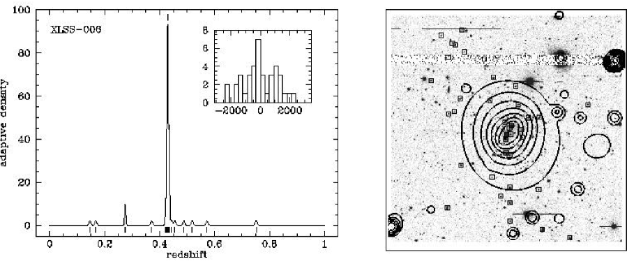
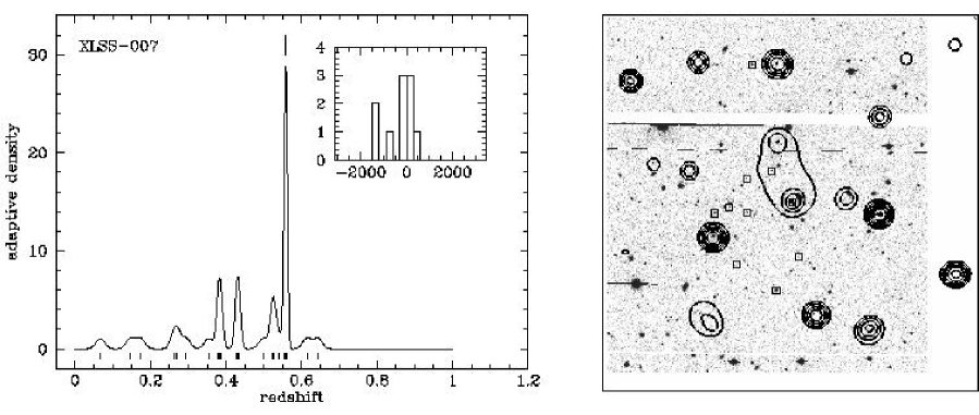
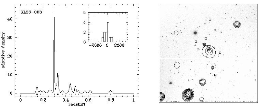
Figure 1: Optical images, X-ray contours and spectroscopic information for each cluster presented in Table 4. Left panel: adaptively smoothed density profile versus redshift. Individual redshifts are marked by short vertical lines below the density curve. A short vertical line above the density curve marks the redshift location of the cluster. The inset histogram displays the rest–frame velocity distribution of confirmed cluster members. Right panel: a $7\arcmin\times 7\arcmin$ $R$–band image centred on the extended X-ray source. Wavelet filtered X-ray contours are overplotted and squares indicate the position of confirmed cluster members. The X-ray contours typically run from two times the background level in each frame to 5 photons/pixel with 10 logarithmic levels. Note that the optical images form a heterogeneous data set and are presented to indicate the visual appearance of each cluster. All optical images are orientated with North up and East left. Where more than one cluster is detected in the same field a black arrow indicates the location of cluster being considered.

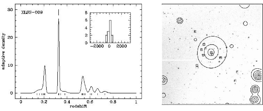
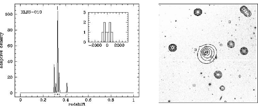
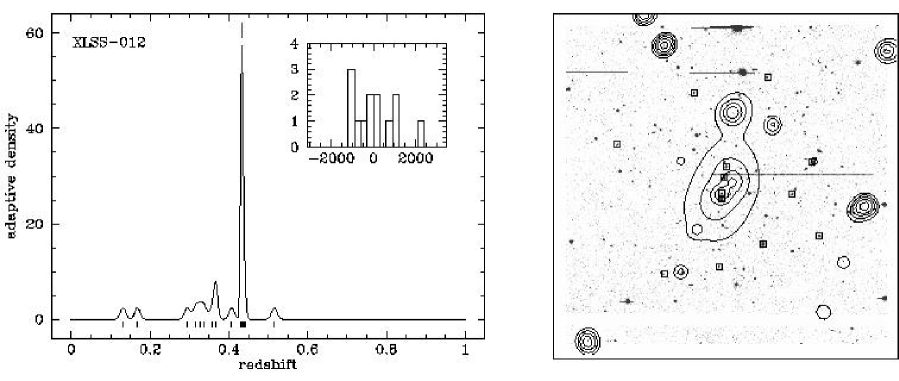
Figure 1: Continued.

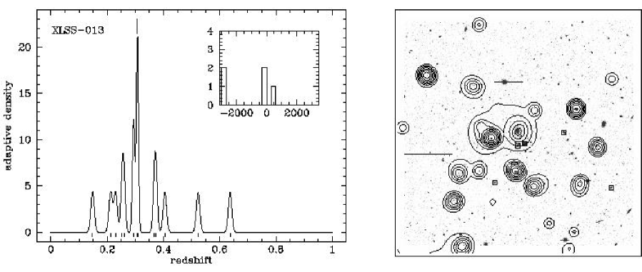
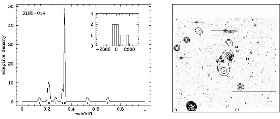
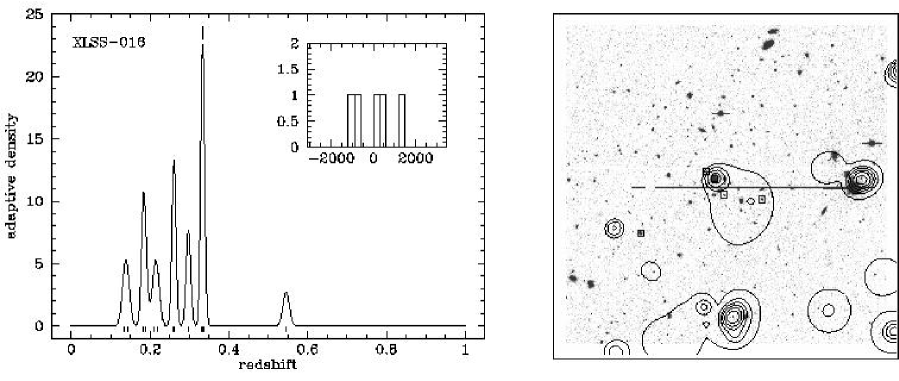
Figure 1: Continued.

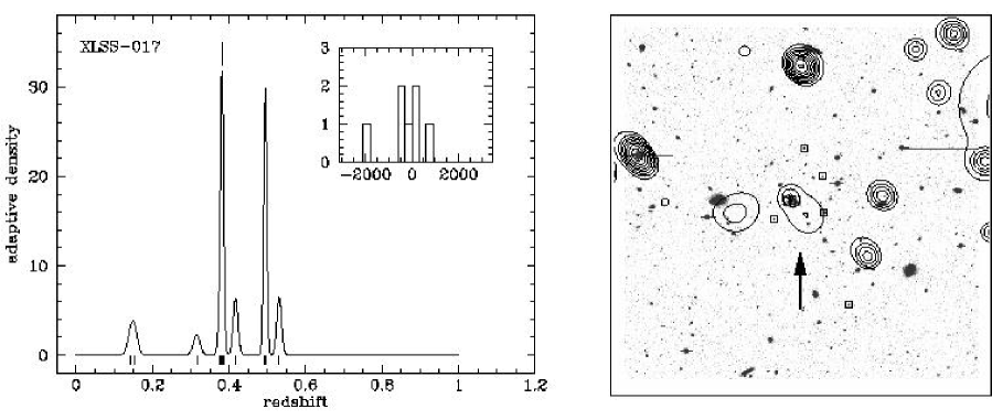
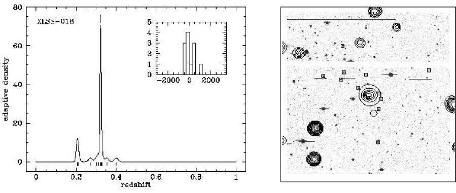
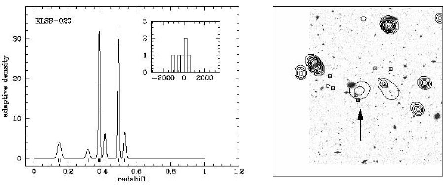
Figure 1: Continued.

The sample of cluster members is selected in radial velocity space employing an iterative method similar to that of Lubin, Oke & Postman (2002): the initial cluster sample is selected to lie within the redshift interval $\Delta z=\pm 0.06$ of the estimated cluster redshift. Radial velocities relative to the cluster centre are calculated within the cluster rest frame, i.e. $\Delta v=c\,(z-{\bar{z}})/(1+{\bar{z}})$ where $\bar{z}$ is the median redshift within the specified interval. The bi–weight mean and scale of the radial velocity distribution within this interval is computed using rostat and galaxies that display a velocity difference relative to the central location of greater than $3500\rm kms^{-1}$ or three scale measures, are rejected and the statistical measures recalculated. This procedure is repeated until no further galaxies are rejected. Errors in the bi–weight mean and scale are estimated employing a bootstrap or jacknife calculation with 10,000 resamplings for clusters with greater than or less than 10 confirmed members respectively. Estimates of the bi–weighted mean radial velocity and line–of–sight velocity dispersion of each cluster, and the associated uncertainties, are corrected for biases arising from measurement errors employing the prescription of Danese et al. (1980).

Although galaxy redshift and positional information is compared to the location of the X–ray source to define the initial cluster redshift input to the velocity search algorithm, no additional spatial filtering of potential galaxy cluster members is performed. However, the projected transverse distances sampled by the detector fields of view employed to perform the spectroscopy vary between 1.5 and 2 $h^{-1}$ Mpc for clusters located over the redshift interval $0.3<z<0.6$. Studies of velocity dispersion gradients in both local (Girardi et al. 1996) and distant (Borgani et al. 1999) X–ray clusters – albeit hotter/more luminous systems than those presented in the current paper – indicate that integrated velocity dispersion profiles typically converge within radii $r<1-2\,h^{-1}$ Mpc of the X–ray cluster centre. Upon initial inspection, the cluster regions sampled by the projected field of view sampled by each telescope plus spectrograph combination would appear to be well matched to the convergent velocity profile of typical hot/luminous clusters. However, inspection of Figure 1 indicates that cluster galaxies are typically confirmed within the central regions in each field – a strategy required by the necessity to confirm the redshift of galaxy structures near the X–ray source. Though the XMM–LSS clusters presented in this paper are typically cooler (i.e. less massive) than those presented by Girardi et al. (1996) and Borgani et al. (1999), and may reasonably be assumed to be intrinsically less extensive, an unknown and potentially significant uncertainty is associated with the assumption that the computed velocity dispersion figures represent the convergent velocity dispersion for each cluster. The resulting spectroscopic properties of all cluster candidates listed in Table 2 are given in Table 4.

Table 4: Spectroscopic properties of all redshift $z<0.6$ groups and clusters

. Cluster Redshift # of members $\sigma_{v}$ ($\rm kms^{-1}$) XLSSC 006 0.429 39 $821_{-74}^{+92}$ XLSSC 007 0.558 10 $323_{-191}^{+178}$ XLSSC 008 0.298 11 $351_{-35}^{+98}$ XLSSC 009 0.327 13 $232_{-31}^{+60}$ XLSSC 010 0.329 8 $420\pm 72$ XLSSC 012 0.433 13 $694_{-91}^{+204}$ XLSSC 013 0.307 5 N/A XLSSC 014 0.344 8 $416\pm 246$ XLSSC 016 0.332 5 $703\pm 266$ XLSSC 017 0.382 7 $571\pm 282$ XLSSC 018 0.322 12 $342_{-35}^{+104}$ XLSSC 020 0.494 6 $265_{-146}^{+240}$

5 Determination of group and cluster X–ray properties

In order to determine the nature of the spectroscopically confirmed clusters presented in this paper, additional analyses of the available XMM data were performed to characterise the spatial and spectral properties of the X–ray emitting gas. When combined with the optical redshift and line–of–sight velocity dispersion (where available) information, these X–ray measures permit a comparison of the cluster sample with lower redshift samples and in particular permit the approximate mass interval occupied by $z<0.6$ XMM–LSS clusters to be understood.

5.1 Morphological properties

The X–ray surface brightness distribution of each cluster was modelled employing a circular $\beta$-model, of the form

$${f(r)=\frac{A}{[1+(r/r_{0})^{2}]^{\,\alpha}},}$$ (1)

where the coordinate $r$ is measured in arcseconds with respect to the centre of the X-ray photon distribution, $r_{0}$ is the core radius, $A$ is the amplitude at $r=0$, and $\alpha=3\,\beta-\frac{1}{2}$.

Images and exposure maps for each cluster field were created for the three EPIC instruments (MOS1, MOS2 and pn) separately in the [0.5–2] keV energy band. Images of the appropriate PSF were created (using SAS-calview), with the appropriate energy weighting together with the off-axis and azimuthal angles of the source. Square regions (of sizes ranging between 175^′′ and 500^′′ on a side) were selected around each source and around a nearby, source-free, background region. Mask images were also created and employed to remove from further analysis regions associated with chip gaps and serendipitous point sources lying close to each cluster source.

We used the Sherpa package from the CIAO analysis system to fit a model of the form given by Equation 1 to the X–ray data for each EPIC instrument. The quality of fit to the three instruments was optimised using the Cash statistic, providing a maximum likelihood fit, which accounts properly for the Poissonian nature of the data. Each model incorporates a flat background model (where the background level is determined employing the associated background region) and a $\beta$–model convolved with the appropriate PSF. For each of the three instrument models determined for each cluster, the values of the core radius $r_{0}$, position ($x_{0}$, $y_{0}$), and slope $\alpha$ were constrained to be identical. Only the normalisation for each model was permitted to vary.

Table 5 lists the best–fit structural parameters for each of the confirmed cluster sources. Figure 2 shows flux contours corresponding to the best–fitting surface brightness model overplotted on the X–ray emission for each candidate. The most interesting outcome from these fits is the low value of the fitted $\beta$ parameter for many of these systems, compared with the typical value of $\beta=0.66$ determined for clusters (Arnaud & Evrard 1999). The median value of $\beta=0.45$ found here agrees with the value of 0.46 derived for a sample of low redshift groups by Heldson & Ponman (2000). Table 5 also lists the value of the normalised $\chi^{2}$ statistic computed from a comparison of the best fitting model to the radially averaged surface brightness profile for each source. The value of the $\chi^{2}$ statistic for each cluster generally indicates that the computed model provides a statistically acceptable fit. The two systems with computed $\chi^{2}$ values significantly less than one (14 and 16) display some of the lowest count levels in the sample and, in these cases, the radially averaged counts may be better described by a Poissonian rather than Gaussian noise distribution – partially invalidating the application of a $\chi^{2}$ merit function.

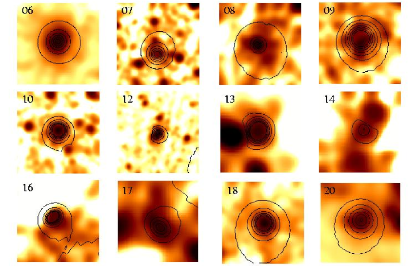
Figure 2: Model surface brightness distributions for the X–ray group and cluster sample. Contours represent the best–fitting model convolved with the detector response and are overplotted on the full (pn$+$MOS1$+$MOS2) Gaussian smoothed X–ray emission corresponding to the [0.5–2] keV energy band. The Gaussian smoothing scale (i.e. the standard sigma) is 5 pixels or 12$\aas@@fstack{\prime\prime}$5.The linearly spaced contours represent the MOS1 model (only the normalisation varies between the three instrument models), except for XLSSC 007 and 013, where the pn model is displayed. The images are of size ’boxside’ (see Table 5).

Table 5: Morphological X–ray parameters determined for confirmed groups and clusters. Displayed errors are $1\sigma$ and, in the case of cluster 19, no reliable error information could be determined. Values of $\chi^{2}$ were computed over a sum of radial bins for each cluster. These values are provided to indicate the overall merit of each fit.

Cluster	boxside	$r_{0}$	$\beta$	$\chi^{2}$
	arcsec	arcsec		(per d.o.f.)
XLSSC 006	250	$24.0_{-2.4}^{+3.1}$	$0.58_{-.02}^{+.04}$	1.34
XLSSC 007	400	$24.0_{-16.0}^{+14.0}$	$0.40_{-.06}^{+.07}$	1.15
XLSSC 008	250	$9.6_{-6.0}^{+8.7}$	$0.44_{-.06}^{+.09}$	1.26
XLSSC 009	250	$44.0_{-19.0}^{+52.0}$	$0.67_{-.17}^{+.73}$	0.96
XLSSC 010	400	$8.5_{-2.6}^{+3.3}$	$0.44_{-.02}^{+.03}$	1.68
XLSSC 012	500	$29.2_{-7.2}^{+10.0}$	$0.54_{-.48}^{+.08}$	1.39
XLSSC 013	175	$11.8_{-6.2}^{+14.9}$	$0.67_{-.16}^{+.67}$	1.34
XLSSC 014	175	$4.7_{-4.7}^{+39}$	$0.40_{-.16}^{+.20}$	0.57
XLSSC 016	200	$2.5_{-2.4}^{+3.5}$	$0.45_{-.07}^{+.10}$	0.79
XLSSC 017	200	$12.1_{-12.0}^{+7.6}$	$0.55_{-.26}^{+.04}$	1.11
XLSSC 018	250	$5.2_{-2.8}^{+3.4}$	$0.42_{-.03}^{+.03}$	1.14
XLSSC 020	200	$24.8_{-22.2}^{+8.1}$	$0.40_{-.16}^{+.04}$	0.99

5.2 Spectral properties

X–ray spectra for each cluster were extracted within a source circle of radius ranging between 30^′′ and 90^′′. The corresponding background spectrum was extracted from a surrounding annulus. Sources adjacent to the cluster were flagged and removed from the spectral analysis employing the source region file generated by the original source extraction software. Source mapping used the stacked pn $+$ MOS1 $+$ MOS2 image of each cluster field in the [0.5-2] keV band only. The source extraction and background regions applied to XLSSC 013 is shown in Figure 3 as an example of the procedure.

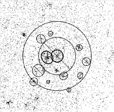
Figure 3: Source and background extraction regions applied to XLSSC 013. The greyscale shows the photon map generated by the stacked pn $+$ MOS1 $+$ MOS2 image.The central solid circle represents the source extraction region. Solid circles crossed with a diagonal line indicate regions excluded from the source aperture. The two large concentric dashed circles define the background annulus and dashed circles crossed with diagonal lines indicate regions excluded from the background aperture.

Extracted spectral data corresponding to pn $+$ MOS1 $+$ MOS2 detectors were fitted simultaneously. The fitting model consists of an absorbed APEC hot plasma model (Smith et al. 2001) with a metal abundance ratio set to Grevesse and Sauval (1999) values. The hydrogen absorption is modeled using a wabs model with $N_{H}$ fixed at the Galactic value, i.e. $\rm N_{H}\sim 2.6\times 10^{20}$ cm^-2. Spectral data are resampled such that the associated background spectrum displays 5 counts per bin and model values are compared to the data by computing the corresponding value of the C–statistic (see Appendix A for a justification for this approach). Model fitting is performed in two stages; first the temperature and abundance are fixed ($T=0.5$ keV, $Z/Z_{\odot}=0.3$) and only the count normalization is fitted. Once a best–fitting spectrum normalisation has been computed, the best–fitting temperature is computed assuming a fixed metal abundance. The fitting results are displayed in Table 6. Table 6 also shows the value of the normalised C–statistic computed from a comparison of the spectral data for each cluster to the quoted model. In each case a statistically reasonable agreement is obtained. Spectral data for all clusters possessing a fitted temperature in Table 6 are displayed in Figure 4. In the cases of clusters 7, 14, 16, 17 and 20, no spectral fit was possible and a temperature of 1.5 keV (typical of the sample as a whole) was assumed for the purpose of calculating the flux from the system.

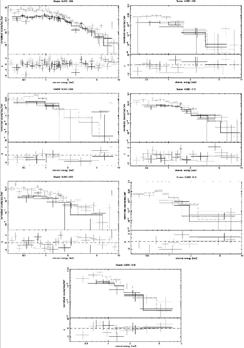
Figure 4: Spectral data for groups and clusters described in Table 6 for which a temperature was fitted. For each system the upper panel depicts the spectral photon flux for the MOS1 (thick black crosses), MOS2 (thin black crosses) and pn (grey crosses). The data have been resampled to 20 photons per spectral bin for display purposes only. The spectral model applicable to each detector is also shown by the appropriately coloured solid line, i.e. MOS1 (solid black line), MOS2 (dotted black line) and pn (grey dashed line). The lower panel shows the deviation of the data from the model for each detector expressed in units of normalised $\chi^{2}$ per spectral bin.

X–ray luminosities for each cluster source have been determined within a uniform physical scale derived from the cluster overdensity radius. In the present study we employ the radius $r_{500}$, within which the total mean density of the system is 500 times the critical density of the universe at the redshift of the system. The value of $r_{500}$ is computed using an isothermal $\beta$–model (Ettori 2000) and employing the fitted gas temperature and $\beta$ value for each system.

We have compared the value of $r_{500}$ derived from the above isothermal model for each cluster to the corresponding values obtained using the observed relationship between cluster mass and temperature. Employing the data presented by Finguenov, Reiprich and Böhringer (2001), based on systems ranging from $T_{X}=0.75-14$ keV, we obtain the following relation

$${r_{500}=0.391\,T_{X}^{0.63}\,h_{70}(z)^{-1}\;\rm Mpc,}$$ (2)

where $h_{70}(z)$ describes the redshift evolution of the Hubble parameter (scaled to 70 kms^-1 Mpc^-1) in the assumed cosmological model. The value for $r_{500}$ for each cluster derived using the above methods typically agree to within $\pm 10$% with the maximal difference being $\pm 20$%. Based upon this comparison we employ $r_{500}$ values based upon the isothermal model in the rest of this paper.

In those cases where a successful spectral fit was obtained, the derived bolometric source flux was extrapolated to $r_{500}$ using the $\beta$–model determined in Section 5.1. For the four systems with detected flux but with no successful spectral fit, the corresponding best–fitting spatial model was employed to compute the bolometric flux within $r_{500}$, assuming a $T=1.5$ keV emission spectrum. Uncertainties on the resulting value of bolometric luminosity are available only for those systems with spectral fits, in which cases the uncertainty is simply derived from the error on the fitted spectral model normalisation. Computation of luminosity uncertainties employing this method does not include the effects of the uncertain extrapolation of the surface brightness model to $r_{500}$. The aperture correction factor for each cluster, $A$, defined as the relative change in the integrated $\beta$–model profile obtained by varying the integration limit from $r_{spec}$ to $r_{500}$, is shown in Table 6.

Table 6: Spectral X–ray parameters determined for confirmed groups and clusters. Values for exposure time, $t_{exp}$, and total counts are summed over all three detectors. Where the letter “F” follows a tabulated temperature (T) value, this indicates that the value was fixed in the fitting procedure. The definition of the aperture correction factor, $A$, is provided in the text. Displayed errors are $1\sigma$.

Cluster	$t_{exp}$	total	$r_{spec}$	T	C–stat	$r_{500}$	$A$	$L_{bol}(r_{500})$
	seconds	counts	arcsec	keV	(per d.o.f.)	Mpc		$\times 10^{43}\;\rm ergs\,s^{-1}$
XLSSC 006	17789	1943	82.5	$4.80_{-0.84}^{+1.12}$	0.85	0.809	1.29	$36.2\pm 2.3$
XLSSC 007	28094	138	90	1.5F	1.10	0.284	0.65	1.1
XLSSC 008	32358	94	60	$1.25_{-0.38}^{+1.44}$	1.04	0.393	1.62	$0.5\pm 0.2$
XLSSC 009	10709	112	90	$0.91_{-0.17}^{+0.20}$	1.12	0.292	0.93	$1.1\pm 0.3$
XLSSC 010	22635	505	67.5	$2.40_{-0.53}^{+0.82}$	1.00	0.539	1.50	$4.6\pm 0.5$
XLSSC 012	37726	635	60	$2.00_{-0.51}^{+1.28}$	1.20	0.462	1.52	$3.0\pm 0.4$
XLSSC 013	34383	133	35	$1.03_{-0.25}^{+0.18}$	0.92	0.437	1.38	$0.5\pm 0.1$
XLSSC 014	14801	286	50	1.5F	1.26	0.404	1.59	0.4
XLSSC 016	27202	25	30	1.5F	0.99	0.432	1.76	0.4
XLSSC 017	25506	79	30	1.5F	1.14	0.456	1.50	0.6
XLSSC 018	62573	295	45	$2.66_{-0.91}^{+2.47}$	1.40	0.558	2.32	$1.3\pm 0.2$
XLSSC 020	16770	61	37.5	1.5F	1.09	0.305	1.01	2.0

6 The nature of XMM–LSS survey selected groups and clusters at $z<0.6$

In this section we compare the properties of the XMM–LSS groups and clusters at $z<0.6$ with X–ray group and cluster samples in the literature. Figure 5 compares the $L_{X}$ versus $T_{X}$ distribution of XMM LSS clusters confirmed at $z<0.6$ to both the distribution formed by the Group Evolution Multi–wavelength Study (GEMS) sample of local ($z<0.03$) X–ray emitting galaxy groups (Osmond and Ponman 2004; hereafter OP04) and the sample of Markevitch (1998; hereafter M98) containing clusters at $z<0.09$ with ASCA temperatures and ROSAT luminosities. Figure 5 indicates that XMM–LSS clusters occupy a region of the $L_{X}$ versus $T_{X}$ plane ranging from cool ($T_{X}>0.9$ keV), low luminosity ($L_{X}(r_{500})>4\times 10^{42}$ ergs s^-1) X–ray groups to moderate temperature ($T_{X}=5$ keV), moderate luminosity ($L_{X}(r_{500})=4\times 10^{44}$ ergs s^-1) clusters. Though the sample of X–ray systems presented in this paper is not statistically complete, it is representative of the properties of the complete flux–limited sample currently under construction. Due to the steeply rising nature of the XLF toward faint X–ray systems, it is anticipated that the larger, statistically complete sample of X–ray structures identified by XMM–LSS at $z<0.6$ will be dominated by such galaxy group and low mass cluster systems.

Figure 5: Distribution of X–ray luminosity computed within a scale radius $r_{500}$ and temperature for all XMM–LSS groups and clusters currently identified at $z\leq 0.6$ (solid squares). Also indicated are values of X–ray luminosity and temperature determined for the low redshift group sample of OP04 (open squares) and for the cluster sample of Markevitch (1998) (open triangles). The solid line indicates an orthogonal regression fit to the $L_{X}$ versus $T_{X}$ relation for both the group and cluster sample incorporating a treatment of the selection effects present in each sample (Heldson and Ponman 2005) – see text for details.

It can be seen from Figure 5, that our XMM–LSS groups and clusters appear to be in good agreement with a linear fit to the $L_{X}$ versus $T_{X}$ distribution of lower redshift group and cluster samples. The local fit to the $L_{X}$ versus $T_{X}$ distribution takes the form $\log L_{X}=2.91~{}\log T_{X}+42.54$ and is derived from an orthogonal regression fit to the combined OP04 plus M98 samples incorporating a treatment of the selection effects present in each sample (Heldson and Ponman 2005). The comparison of XMM–LSS groups and clusters to this local relationship may be quantified (Figure 6) by calculating a luminosity enhancement factor, $F=L_{obs}/L_{pred}$, where $L_{obs}$ is the observed cluster X–ray luminosity within a radius, $r_{500}$, and $L_{pred}$ is the luminosity expected applying the fitted $L_{X}$ versus $T_{X}$ relation computed for the local fit and the XMM–LSS measured temperature. Neglecting the 5 systems assigned a fixed temperature (XLSSC 007, 014, 016, 017 and 020 – for which the temperature uncertainty is unknown) , the median enhancement factor of the remaining 6 systems is $F=1.09$. For comparison, the expected enhancement in $L_{X}$ due to self-similar evolution, scaling to $r_{500}$, is a factor of 1.23 at the typical redshift ($z=0.4$) of our sample. Therefore, given the observed spread in the enhancement values, the observed negative deviation from the self–similar expectation is not large.

Given the modest size and the statistically incomplete nature of our current sample, we regard these results as in need of confirmation. Ettori et al. (2004) also report evolution weaker than the self–similar expectation from a sample of 28 clusters at $z>0.4$ with gas temperatures $3~{}{\rm keV}<T<11~{}{\rm keV}$. The combined effect of self–similar scaling with the negative evolution reported by Ettori et al. (2004) would result in an enhancement factor $F=0.86$ at a $z=0.4$ (see Figure 6). Though the overlap of the Ettori et al. (2004) sample and the systems contained in the present work is limited, the X–ray luminosities appear to describe similar trends.

Figure 6: Enhancement factor, $F=L_{obs}/L_{pred}$, computed for six XMM–LSS groups and clusters located at $z\leq 0.6$ plotted versus the X–ray temperature of each system (see text for additional details). Horizontal lines indicate expected values of $F$: the short dashed line indicates the value $F=1.23$ expected from self–similar considerations. The dotted line indicates the value of $F$ expected at $z=0.4$ based upon Ettori et al. (2004).

The relationship between the specific energy contained within the cluster galaxy motions, compared to the X–ray emitting gas, is described via the $\beta_{spec}$ parameter

$${\beta_{spec}\equiv\frac{\sigma_{v}^{2}}{kT_{X}/\mu m_{p}}}$$ (3)

where $\sigma_{v}$ is the line–of–sight galaxy velocity distribution, $k$ is the Boltzmann constant, $T_{X}$ is the X–ray gas temperature and $\mu m_{p}$ is the mean particle mass within the gas (Bahcall & Lubin 1994). Figure 7 displays the value of $\beta_{spec}$ computed for the XMM–LSS $z<0.6$ cluster sample as a function of computed X–ray luminosity extrapolated to a radius $r_{500}$ (i.e. the consistent measure adopted in this paper). A number of systems have been excluded from Figure 7: in addition to the systems excluded from the computation of the luminosity enhancement factor above, XLSSC 013 does not possess well defined galaxy velocity dispersion thus preventing computation of $\beta_{spec}$. Figure 7 indicates typical values $\beta_{spec}<1$ for the XMM–LSS $z<0.6$ sample (with the exclusion of the above mentioned systems), the median value of $\beta_{spec}$ for this restricted sampled is $\langle\beta_{spec}=0.61\rangle$. This value may be compared to values of $\beta_{spec}\approx 1$ reported by OP04 for luminous X–ray groups (i.e. $L_{X}(r_{500})>10^{42}$ ergs s^-1).

Figure 7: Values of $\beta_{spec}$ computed for eight XMM–LSS groups and clusters at $z\leq 0.6$ (see text for details) plotted versus the X–ray luminosity for each system. The horizontal dashed line indicates the value $\beta_{spec}=1$.

A clear concern when interpreting the trend of low $\beta_{spec}$ values is the extent to which the cluster galaxy velocity dispersion estimates may be biased toward lower values. Potential uncertainties associated with the velocity dispersion values presented in this paper are discussed in Section 4. However, in the overwhelming majority of clusters observed in detail, the integrated velocity dispersion profile of galaxy clusters is a decreasing function of projected radius from the cluster centre (Girardi et al. 1996; Borgani et al. 1999). If the integrated velocity dispersion profiles of the XMM–LSS clusters presented in this paper display similar behaviour to hotter clusters, then the expectation arising from computation of the cluster velocity at some fraction of the convergent radius is that the velocity dispersion will be overestimated and will result in values of $\beta_{spec}$ biased to higher values. The extent of any such bias is difficult to quantify in the current data set. However, the implication is that the value of $\beta_{spec}$ displayed in Figure 7 would not increase with the addition of velocity dispersion measurements extending to larger radii.

The low values of $\beta_{spec}$ apparent in Figure 7, are similar to those seen by OP04 in lower luminosity groups ($L_{X}<10^{42}$ ergs s^-1) at low redshift. The origin of these low values of $\beta_{spec}$ is far from clear, but OP04 argue that it appears to result primarily from a reduction in $\sigma_{v}$, rather than an enhancement in $T_{X}$. Whatever the cause, our results provide tentative evidence that these effects are operating in hotter and more X–ray luminous systems at higher redshift. We are currently in the process of conducting magnitude limited spectroscopy of a sample of $T_{X}\sim 1$ keV systems at $z=0.3$ in order to provide a more robust picture of the dynamics of low temperature X–ray systems.

7 Conclusions

We have presented twelve newly identified X–ray selected groups and clusters as part of the XMM Large–scale Structure Survey. The procedures employed to detect and classify sources in X–rays, and to subsequently confirm each source via optical imaging and spectroscopic observations have been described in detail.

We have emphasized throughout this paper that the current sample of clusters is not complete in any statistical sense. The presentation of a larger, complete sample of X–ray clusters located at $z<0.6$ will form part of a future publication. However, the current sample of X-ray clusters at $z<0.6$ presents a number of interesting features: most importantly, the sample is dominated by low X–ray temperature systems located at redshifts much greater than that presented by previous X–ray studies. Such systems are predicted to display the effects of pre–heating or additional energy input into the ICM to a greater extent than hotter, more massive systems. The identification of such low–temperature systems at look–back times up to 5.7 Gyr provides an important baseline over which to study the extent to which such systems evolve.

We find tentative evidence that these high redshift groups are more luminous than local systems, at a given temperature, in agreement with recent work on richer clusters. However, our results suggest that group luminosities may be evolving less rapidly than higher temperature clusters when compared to self-similar models. If this is confirmed to be the case, then the steepening of the $L_{X}$-$T_{X}$ relation at low temperatures reported in local samples, may continue at higher redshift. We also find preliminary indications that the poorly understood tendency for the specific energy in the gas to exceed that in the galaxies in poor groups, extends to systems with higher values of $L_{X}$ and $T_{X}$ at $z\sim 0.4$. The completion of a larger and statistically complete sample of intermediate redshift groups from the XMM–LSS survey, should allow these results to be placed on a firm statistical footing in the near future.

Appendix A Fitting simulated cluster spectra

The current study extends X–ray spectral observations of distant galaxy groups and clusters to low integrated signal levels ($\sim 100$ photons above the background).It is therefore prudent to assess the reliability of temperature measures and associated uncertainties computed via model fits to such faint spectra by repeating the fitting procedure for a grid of simulated spectra created to reproduce the properties of the observed sample.

The source model used to simulate group and cluster spectra employs an APEC of an optically thin plasma (Smith et al. 2001). This model depends upon four parameters: temperature, metal abundance, redshift and a normalisation representative of the emission integral. To simulate galaxy groups and clusters the abundance is set to $Z/Z_{\odot}=0.3$ with solar abundance ratios set to Grevesse and Sauval (1999) values. The redshift of the simulated source is set to $z=0.3$, typical of the sources presented in this paper. Photoelectric absorption described by a wabs model within Xspec using Morrison and McCammon (1983) cross–sections was applied to the source model with the neutral hydrogen column density fixed to $\rm N_{H}=2.6\times 10^{20}~{}cm^{-2}$ – the mean value for our sample according to the HI distribution map of Dickey and Lockman (1990). The instrumental response was modeled using the redistribution matrix and ancillary response files from observations of XLSSC 006.

A model pn $+$ MOS1 $+$ MOS2 spectra was created and a conversion factor applied to generate spectra of the required integrated count level over the spectral interval [0.3–10] keV in a 10,000 second exposure. Each simulated spectrum is generated from this model using Poissonian considerations. Each source spectrum is accompanied by a background spectrum created from a Poisson realisation of a background model of normalisation and shape consistent with observed cluster backgrounds. Spectra were simulated according to this procedure for temperatures equal to $1,2,3$ and 5 keV. At each temperature, 50 spectra were simulated at each point of a grid of integrated count levels $100,200,\dots,1000$.

Spectral fitting follows the same approach as applied to observed data, i.e. temperature and spectum normalisation are permitted to vary while the abundance is fixed. Data from pn $+$ MOS1 $+$ MOS2 are are combined within Xspec with the response files from XLSSC 006 and the energy range [0.3–10] keV is conserved. The spectral energy range corresponding to [7.5–8.5] keV measured by the pn detector is ignored as it contains strong instrumental line emission that is not well corrected by our data modeling process. The best–fitting model is then determind by minimising a modified C–statistic and the $1~{}\sigma$ uncertainty about the best fit model is computed. While the C–statistic is intended to work efficiently on unbinned data a comparison of the fitted temperature to the input value indicates a tendency to underestimate the temperature of spectra of input temperatures $<5$ keV displaying count values $<1000$ counts using this procedure. This bias is indicated in Figure 8 and appears to arise from the fact that the statistic used in Xspec represents a modified C–statistic that accounts for statistical fluctuations in the background estimation. Our understanding of the problem is that this modified statistic fails at estimating model parameters when there is a significant number of background bins containing zero photons.

Resampling the data to prevent the occurence of spectral bins containing zero counts minimises this negative temperature bias. The resampling factor is determined by requiring that the background spectrum associated with each source display a specified minimum count level per spectral bin. Determining the resampling factor from the background spectrum represents a sensible approach as the background counts are more numerous and therefore minimise the loss of spectral information in the source spectrum. Although a small positive bias is introduced to the fitted temperatures of very low count level spectra ($<300$ counts) when the data are resampled, the amplitude of this bias is less than 10% when the data are resampled to contain 5 counts per spectral bin (Figure 8). Applying a larger resampling factor increases the positive temperature bias – which can be understood in terms of the spectral smoothing that the resampling procedure represents.

We therefore resample the observed data to generate a background spectrum containing 5 counts per spectral bin. This approach generates fitted temperatures that agree with the input temperature to $<10$%. In addition, comparison of the distribution of fitted temperatures at any given combination of temperature and count level to the temperature uncertainty returned by Xspec indicates that the Xspec quoted errors on fitted temperatures overestimate the distribution of fitted temperatures by a factor typically less than 2. Due to the various assumptions that enter the simulation procedure it therefore seems reaonable to provide Xspec quoted temperature uncertainties as a conservative error estimate.

Figure 8: A comparison of Xspec computed temperatures for simulated group and cluster spectra employing the C–statistic with two different resampling approaches. Left panels indicate the results for unbinned spectra. Right panels indicate the results for binned spectra such that the background spectrum displays a minimum of 5 counts per spectral bin. Panels in each row correspond to spectral models with the indicated input temperature (also shown by the horizontal dashed line). In each panel, data points represent the mean Xspec computed temperature returned from the set of simulated spectra as a function of total input counts. Filled squares plus error bars indicate the mean computed temperature and the distribution of temperatures accounting for 68% of the sample. Open squares plus error bars indicate the mean computed temperature and the median $1~{}\sigma$ uncertainty returned by Xspec (open squares are shifted to the right by 30 counts with respect to the filled squares for clarity).

References

- (1) Andreon, S., Ettori, S., 1999, ApJ, 516, 647
- (2) Andreon, S., Willis, J., Quintana, H., Valtchanov, I., Pierre, M., Pacaud, F., 2004a, MNRAS, 353, 353
- (3) Andreon, S. et al., 2004b, MNRAS, 539, 1250
- (4) Allen, S., Schmidt, R., Fabian, A., Ebeling, H., 2003, MNRAS, 342, 287
- (5) Arnaud, M., Evrard, A., 1999, MNRAS, 305, 631
- (6) Bahcall, N., Lubin, L., 1994, ApJ, 426, 513
- (7) Baugh, C., Cole, S., Frenk, C., 1996, MNRAS, 283, 1361
- (8) Beers, T., Flynn, K., Gebhardt, K., 1990, AJ, 100, 32
- Bertin & Arnouts (1996) Bertin, E., Arnouts, S., 1996, A&AS, 117, 393
- (10) Böhringer, H., Collins, C., Guzzo, L., Schuecker, P., Voges, W., Neumann, D. M., Schindler, S., Chincarini, G., De Grandi, S., Cruddace, R. G., Edge, A. C., Reiprich, T. H., Shaver, P., 2002, ApJ, 566, 93
- (11) Borgani, S., Girardi, M., Carlberg, R., Yee, H., Ellingson, E., 1999, ApJ, 527, 561
- (12) Borgani, S., Rosati, S., Tozzi, P., Stanford, S. A., Eisenhardt, P. R., Lidman, C., Holden, B., Della Ceca, R., Norman, C., Squires, G., 2001, ApJ, 561, 13
- (13) Bryan, G.L., Norman, M.L., 1998, ApJ, 495, 80
- (14) Burke, D., Collins, C., Sharples, R., Romer, A. K., Holden, B. P., Nichol, R. C., 1997, ApJ, 488, 83
- (15) Danese, L., de Zotti, G., di Tullio, G., 1980, A&A, 82, 322
- (16) Dickey, J.M., Lockman, F.J., 1990, ARA&A, 28, 215
- (17) Dressler, A., Smail, I., Poggianti, B., Butcher, H., Couch, W. J., Ellis, R. S., Oemler, A., Jr., 1999, ApJS, 122, 51
- (18) Ebeling, H., Edge, A., Henry, J., 2001, ApJ, 553, 668
- (19) Ettori, S., Tozzi, P., Borgani, S., Rosati, P., 2004, A&A, 417, 13
- (20) Ettori, S., 2000, MNRAS, 311, 313
- (21) Evrard, A.E., 2004, Clusters of Galaxies: Probes of Cosmological Structure and Galaxy Evolution, from the Carnegie Observatories Centennial Symposia. Published by Cambridge University Press, as part of the Carnegie Observatories Astrophysics Series. Edited by J.S. Mulchaey, A. Dressler, and A. Oemler, p. 1.
- (22) Finoguenov, A., Reiprich, T. H., Böhringer, H., 2001, A&A, 368, 749
- (23) Evrard, A.E., Metzler, C.A., Navarro, J.F., 1996, ApJ, 469, 494
- (24) Girardi, M., Fadda, D., Giuricin, G., Mardirossian, F., Mezzetti, M., 1996, ApJ, 457, 61
- (25) Grevesse, N., Sauval, A.J., 1999, A&A, 347, 348
- (26) Hamuy, M., Walker, A., Suntzeff, N., 1992, PASP, 104, 533
- (27) Hamuy, M., Suntzeff, N., Heathcote, S., 1994, PASP, 106, 566
- (28) Heavens, A., 1993, MNRAS, 263, 735
- (29) Heldson, S., Ponman, T., 2000, MNRAS, 319, 933
- (30) Heldson, S., Ponman, T., 2003, MNRAS, 339, 29
- (31) Heldson, S., Ponman, T., 2005, MNRAS, in preparation
- (32) Henry, J., Gioia, I., Maccacaro, T., Morris, S. L., Stocke, J. T., Wolter, A., 1992, ApJ, 386, 408
- (33) Kauffman, G., 1996, MNRAS, 281, 487
- (34) Kinney, A., Calzetti, D., Bohlin, R., McQuade, K., Storchi-Bergmann, T., Schmitt, H. R., 1996, ApJ, 467, 38
- (35) Kodama, T., Arimoto, N., Barger, A., Aragon–Salamanca, A., 1998, A&A, 334, 99
- (36) Ledlow, M., Loken, C., Burns, J., Owen, F., Voges, W., 1999, ApJ, 516, L53
- (37) Lubin, L., Oke, B., Postman, M., 2002, AJ, 124, 1905
- (38) Lumb, D., Bartlett, J., Romer, A., Blanchard, A., Burke, D. J., Collins, C. A., Nichol, R. C., Giard, M., Marty, P. B., Nevalainen, J., Sadat, R., Vauclair, S. C., 2003, A&A, 420, 853
- (39) Markevitch, M., 1998, ApJ, 504, 27
- (40) Morrison R., McCammon, D., 1983, ApJ, 270, 119
- (41) McCracken, H., Radovich, M., Bertin, E., Mellier, Y., Dantel-Fort, M., Le Fèvre, O., Cuillandre, J. C., Gwyn, S., Foucaud, S., Zamorani, G., 2003, A&A, 410, 17
- Osmond & Ponman (2004) Osmond, J. P. F., Ponman, T. J., 2004, MNRAS, 350, 1511
- (43) Pacaud, F., et al., 2005, A&A, in preparation.
- (44) Pierre, M., et al., 2004, JCAP, 9, 11
- (45) Ponman, T., Cannon, D., Navarro, J., 1999, Nature, 397, 135
- (46) Refregier, A., Valtchanov, I., Pierre, M., 2002, A&A, 390, 1
- (47) Rosati, P., della Ceca, R., Norman, C., Giacconi, R., 1998, ApJ, 492, 21
- (48) Rosati, P. Borgani, S., Norman, C., 2002, ARA&A, 40, 539
- (49) Sanderson, A., Ponman, T., Finoguenov, A., Lloyd-Davies, E. J., Markevitch, M., 2003, MNRAS, 340, 989
- (50) Schuecker, P., Böhringer, H., Guzzo, L., Collins, C. A., Neumann, D. M., Schindler, S., Voges, W., De Grandi, S., Chincarini, G., Cruddace, R., Möller, V., Reiprich, T. H., Retzlaff, J., Shaver, P., 2001, A&A, 368, 86
- (51) Silverman, B., 1986, Density Estimation for Data Analysis and Statistics (London: Chapman and Hall)
- (52) Smith, R.K., Brickhouse, N.S., Liedahl, D.A., Raymond, J.C., 2001, ApJL, 556,91
- (53) Stanford, S., Eisenhardt, P., Dickinson, M., 1998, ApJ, 492, 461
- (54) Starck, J., Pierre, M., 1998, A&AS, 128, 397
- (55) Tonry, J., Davis, M., 1979, AJ, 84, 1511
- Valtchanov et al. (2001) Valtchanov, I., Pierre, M., Gastaud, R., 2001, A&A, 370, 689
- (57) Valtchanov, I., Pierre, M., Willis, J., Dos Santos, S., Jones, L., Andreon, S., Adami, C., Altieri, B., Bolzonella, M., Bremer, M., Duc, P.-A., Gosset, E., Jean, C., Surdej, J., 2004, A&A, 423, 75
- (58) Vikhlinin, A., McNamara, B., Forman, W., Jones, C., Quintana, H., Hornstrup, A., 1998, ApJ, 498, L21
- (59) Vikhlinin, A., VanSpeybroeck, L., Markevitch, M., Forman, W. R., Grego, L., 2002, ApJL, 578, 107
- (60) Voit, G.M., 2004, Proceedings of The Riddle of Cooling Flows in Galaxies and Clusters of Galaxies, held in Charlottesville, VA, May 31 - June 4, 2003, Eds. T. Reiprich, J. Kempner, and N. Soker.
- (61) Yee, H., Ellingson, E., Carlberg, R., 1996, ApJS, 102, 269